Quantum baker map on the sphere

Abstract

We define a class of dynamical systems on the sphere analogous to the baker map on the torus. The classical maps are characterized by dynamical entropy equal to $\ln 2$. We construct and investigate a family of the corresponding quantum maps. In the simplest case of the model the system does not possess a time reversal symmetry and the quantum map is represented by real, orthogonal matrices of even dimension. The semiclassical ensemble of quantum maps, obtained by averaging over a range of matrix sizes, displays statistical properties characteristic of circular unitary ensemble. Time evolution of such systems may be studied with the help of the $SU(2)$ coherent states and the generalized Husimi distribution.

I Introduction

The classical baker map on the torus is often used to illustrate properties of chaotic dynamical systems [1, 2, 3]. It may be regarded as the simplest generalization of the Bernoulli shift in two dimensions. The baker map is measure preserving and chaotic: it belongs to a small class of the dynamical systems, for which the metric Kolmogorov-Sinai entropy is positive and may be calculated analytically. This classical dynamical system has been generalized in several ways. The generalized baker map was used to study properties of invariant measures and fractal dimensions [4, 5], while snapshot attractors appearing in the random baker map were analyzed in [6, 7]. Another generalization of the model, called multibaker map [8, 9], is useful for investigating the effects of deterministic diffusion. Chaotic dynamics of a classical map can be described as a linear evolution of densities transformed by an associated Frobenius–Perron operator. Much progress has recently been achieved [8, 10, 11, 12, 13, 14] in finding the spectrum and understanding some unusual properties of the right and the left eigenstates of the F–P operator of the classical baker map.

A first attempt to quantize the baker map on the torus is due to Balazs and Voros [15]. Another, more symmetric version of the quantum map was found by Saraceno  [16]. A general construction allowing one to quantize a class of piecewise linear maps on the torus (including the baker map) was given by De Bièvre, Degli Esposti, and Giachetti [17]. While another quantization scheme was recently proposed by Rubin and Salwen [18]. The quantum baker map on the torus become a standard model used to pursue the concept of semiclassical quantization of non-integrable classical systems [19, 20, 21, 22, 23, 24, 25, 27, 28, 29] emerging from the theory of Gutzwiller [30, 31]. In several other papers devoted to the quantum baker map one demonstrated sensitivity of eigenstates of the system with respect to small perturbations [32], proposed an optical realization of this quantum map [33], and designed a scheme of realization of the baker map by methods of quantum computing [34].

In this work we propose a different dynamical system: the baker map on the sphere. In fact we define an entire family of classical systems and the corresponding quantum maps. On one hand, the classical version of this model is, to our best knowledge, the first dynamical system on the sphere with explicitly computable, positive K-S entropy. On the other, analysis of several possible versions of the analogous quantum systems may help in clarifying various aspects of the quantum–classical correspondence for non-integrable dynamical systems.

In the simplest case of the model the map defined on the sphere is not symmetric with respect to the reversal of time. The Floquet operator describing the time evolution of the corresponding quantum map is constructed out of the Wigner rotation matrices and is represented by orthogonal matrices of even dimension. In the general case the evolution operators are represented by complex unitary matrices.

Each quantum model, corresponding to a given classical system, can be generalized by introducing into the model an arbitrary complex phase [15]. One obtains than a one parameter family of quantum maps acting in the same Hilbert space, which may be useful for studying various aspects of level dynamics: curvatures, correlations of velocities and anticrossings.

Phase space features and the time evolution of the quantum map can be suitably analyzed with help of the $SU(2)$ coherent states. A simple generalization of the quantization scheme presented in [15] provides four different maps (with different spectra and traces), that seem to correspond to the same classical system. This quantization scheme allows us to obtain two versions of the symmetric quantum baker map on the torus different from that introduced in [16].

The paper is organized as follows. The quantum version of the baker map on the sphere is introduced in Section II. The corresponding classical system is analyzed in Section III, while the statistical properties of the quantum map are discussed in Section IV. Appendix A contains the proof of unitarity of auxiliary matrices constructed out of the Wigner rotation matrices. Detailed formulae for four versions of the quantum baker map on the sphere are given in Appendix B, while the entire family of the classical and quantum models is given in Appendix C. An analogous construction for the baker map on the torus is shown in Appendix D.

II Construction of the Quantum map

To construct the quantum map corresponding to a given classical transformation on the sphere we use the $N$–dimensional representation of the rotations group. Using the angular momentum operators commutation relation

$$\left[J_{i},J_{j}\right]=i\epsilon_{ijk}J_{k}$$ (1)

we obtain $N=2j+1$ base vectors $|j,m\rangle_{i}$, eigenstates of $J^{2}$ and $J_{i}$ (i-th coordinate of $J$)

$$J^{2}|j,m\rangle_{i}=j(j+1)|j,m\rangle_{i},\ \ \ J_{i}|j,m\rangle_{i}=m|j,m\rangle_{i},$$ (2)

$m=-j,\ldots,j$. To work in an even dimensional Hilbert space ${\cal H}$ we consider the half–integer values of $j$.

We design the quantum baker map $B_{S}$ on the sphere in such a way that $B_{S}$ commutes with $J^{2}$ and the quantum number $j$ is preserved. Therefore it is convenient to simplify the notation by writing $|m\rangle_{i}$ instead of $|j,m\rangle_{i}$. The action of the baker map has to stretch phase space along one direction ($z$-axis) and to squeeze along the other one (say, along the $x$-axis). The transformation between these two basis $|\Psi\rangle_{x}=R|\Psi\rangle_{z}$ is described by the Wigner rotation matrix $R$ [35] representing a rotation around $y$-axes by the angle $\pi/2$. We use its representation in the $|m\rangle_{z}$ basis

$$R_{m^{\prime},m}={}_{z}\langle m|e^{-i\frac{\pi}{2}J_{y}}|m^{\prime}\rangle_{z}$$ (3)

with $m,m^{\prime}=-j,\dots,j$. This matrix is real and has the following property

$$R_{m^{\prime},m}=(-1)^{m-m^{\prime}}R_{m,m^{\prime}}=(-1)^{m-m^{\prime}}R_{-m^{\prime},-m}\ .$$ (4)

Let us split the Hilbert space ${\cal{H}}$ into two subspaces distinguished by its projection on $|m\rangle_{z}$

$${\cal{H}}^{S} = \left\{|\Psi\rangle\in{\cal{H}}:{}_{z}\langle m|\Psi\rangle=0,\ m>0\right\}$$ (5)

$${\cal{H}}^{N} = \left\{|\Psi\rangle\in{\cal{H}}:{}_{z}\langle m|\Psi\rangle=0,\ m<0\right\},$$ (6)

so that ${\cal{H}}^{S}$ contains the states localized on the southern hemisphere and ${\cal{H}}^{N}$ – on the northern one. Projection on $|k\rangle_{x}$ leads to another partition

$${\cal{H}}^{W} = \left\{|\Psi\rangle\in{\cal{H}}:{}_{x}\langle k|\Psi\rangle=0,\ k>0\right\}$$ (7)

$${\cal{H}}^{E} = \left\{|\Psi\rangle\in{\cal{H}}:{}_{x}\langle k|\Psi\rangle=0,\ k<0\right\},$$ (8)

so ${\cal{H}}={\cal{H}}^{S}+{\cal{H}}^{N}={\cal{H}}^{W}+{\cal{H}}^{E}$. The baker map transforms each vector $|\Psi^{S}\rangle\in{\cal{H}}^{S}$ into a vector $|\Phi^{W}\rangle\in{\cal{H}}^{W}$, with a linear stretching by a factor of two in the $z$ direction. The effect of this stretching can be formalized by the condition that the $N/2$ odd (even) coefficients of the state $|\Phi^{W}\rangle$ expanded in the basis $|m\rangle_{z}$ are given by the first $N/2$ coefficients of the state $|\Psi^{S}\rangle$ represented in the same basis

$${}_{z}\langle m|\Psi^{S}\rangle=\sqrt{2}~{}{}_{z}\langle 2m+j|\Phi^{W}\rangle~{}~{}{\rm{for}}~{}~{}m=-j,\dots,-1/2.$$ (9)

The factor $\sqrt{2}$ leads to the correct normalization.

The analogue condition for the linear squeezing in $x$-direction would give the overcomplete system of equations with no solution. This fact is rather intuitive because it is not possible to map the southern hemisphere into the western one with the linear stretching in $z$-direction and the linear squeezing in $x$. However, we require $|\Phi^{W}\rangle$ to be squeezed to the western hemisphere ${\cal{H}}^{W}$

$${}_{x}\langle k|\Phi^{W}\rangle=0\ ~{}~{}{\rm{for}}~{}~{}k=1/2,\dots,j.$$ (10)

The above condition corresponds to a nonlinear squeezing in $x$. We want to find a linear operator $B^{SW}$ which transforms $|\Psi^{S}\rangle$ into $|\Phi^{W}\rangle$

$$|\Phi^{W}\rangle_{z}=B^{SW}|\Psi^{S}\rangle_{z}\ .$$ (11)

To rewrite this formula into the $|k\rangle_{x}$ basis we multiply its both sides by the transformation matrix $R$: $|\Phi^{W}\rangle_{x}=RB^{SW}|\Psi^{S}\rangle_{z}$. To satisfy the condition (10) all elements of the lower half of the matrix $RB^{SW}$ must vanish. Since we want $RB^{SW}$ to act only on the subspace ${\cal{H}}^{S}$ we set to zero the right half of this matrix. Denoting by $M$ the only unknown $N/2\times N/2$ block of the matrix $RB^{SW}$ we put equation (11) in the form

$${}_{z}\langle k|\Phi^{W}\rangle=\sum_{l=-j}^{j}\ \sum_{m=-j}^{j}\ \left[R^{-1}\right]_{k,l}\left[\begin{array}[]{cc}M_{l,m}&0\\ 0&0\end{array}\right]{}_{z}\langle m|\Psi^{S}\rangle\ ,$$ (12)

Inserting above into (9) we obtain the following conditions for the matrix $M$

$$\sqrt{2}\sum_{l=-j}^{-\frac{1}{2}}\ \left[R^{-1}\right]_{2k+j,l}M_{l,m}=\delta_{k,m}\ \ \ \mbox{for}\ \ k,m=-j,\ldots,-\frac{1}{2}\ .$$ (13)

In the appendix A we show that the matrix $R^{\prime}$ composed of half of every even (odd) column of the matrix $\sqrt{2}\,R$ is unitary, (since it is real, it is also orthogonal). Consequently, we take $M_{l,m}=\sqrt{2}\,R_{l,2m+j}=:R^{\prime}_{l,m}$ ($l,m=-j\ldots-1/2$) and insert it into (12) constructing in this way the transformation ${B}^{SW}:\,{\cal{H}}^{S}\rightarrow{\cal{H}}^{W}$. The other matrix $R^{\prime\prime}_{l,m}:=\sqrt{2}\,R_{l,2m-j}$ (now $l,m=1/2\ldots j$) is also unitary, which allows us to build the second transformation ${B}^{NE}:\,{\cal{H}}^{N}\rightarrow{\cal{H}}^{E}$ in the same manner. We define the quantum baker map on the sphere as a linear operator $B_{S}={B}^{SW}+{B}^{NE}$ acting on $\cal{H}$. In the $|m\rangle_{z}$ basis the quantum baker map on the sphere takes the form

$$B_{S}=R^{-1}\left[\begin{array}[]{cc}R^{\prime}&0\\ 0&R^{\prime\prime}\end{array}\right].$$ (14)

In the mixed representation (${}_{z}\langle m|B_{S}|m^{\prime}\rangle_{x}$) the baker map on the sphere consists of two diagonal blocks $R^{\prime}$ and $R^{\prime\prime}$. Figure 1 shows $(B_{S})^{n}$ in this representation for $n=0,1,2,3$. The first plot obtained with $n=0$ displays just the elements of the rotation matrix $R_{m^{\prime}m}={}_{z}\langle m|m^{\prime}\rangle_{x}$. For $m$ and $m^{\prime}$ fulfilling $m^{2}+m^{\prime 2}>j^{2}$ such elements are exponentially small. This fact has a simple classical analogy. Consider a partition of the unit ball into $N$ slices of the same width perpendicular to the direction $z$ and another partition consisting of $N$ slices perpendicular to the direction $x$. Some side $z$-slices (of small radii) do not overlap with some side $x$-slices. This ’circular’ structure manifests itself also in the pictures obtained for $n=1,2$ and $3$ and contrasts with the rectangular patterns visible in the analogous figure drawn by Saraceno and Voros [25] for the quantum map on the torus.

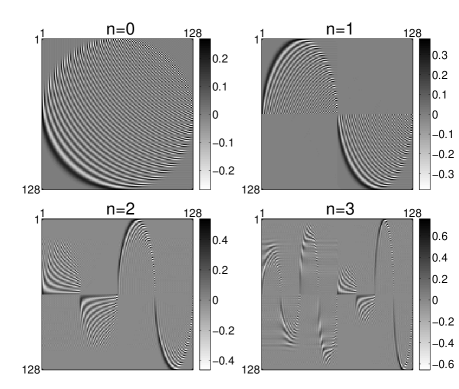
FIG. 1.: Quantized baker map on the sphere $(B_{S})^{n}$ shown in the mixed representation for $N=128$ and $n=0,1,2$ and $3$. Gray tone scale represents values of real elements of $N\times N$ matrices.

The rotation matrix $R$ is unitary, as are the matrices $R^{\prime}$ and $R^{\prime\prime}$, constructed out of its elements. Hence the quantum map $B_{S}$ is unitary. Writing equations (9) describing the double stretching of the vector $|\Psi^{S}\rangle$ we can choose ${}_{z}\langle 2m+j|$ (odd column of $R$) or ${}_{z}\langle 2m+j+1|$ (even column) projections of the state $|\Phi^{W}\rangle$. A similar ambiguity remains in the choice of the vector $|\Phi^{E}\rangle$, so one may construct four different versions of the quantum map: ${B_{S}}^{(00)},{B_{S}}^{(01)},{B_{S}}^{(10)}$ and ${B_{S}}^{(11)}$, as written explicitly in Appendix B. In the classical limit $N\to\infty$ all four families of quantum maps seem to tend to the same classical system.

In order to create one parameter families of quantum maps it is possible to introduce a phase factor $\lambda$ into any of the above four versions of the model

$$B_{S}(\lambda)=R^{-1}\left[\begin{array}[]{cc}e^{i\lambda}R^{\prime}&0\\ 0&e^{-i\lambda}R^{\prime\prime}\end{array}\right].$$ (15)

This particular way of introducing the parameter $\lambda$ is advantageous, since there is no drift of the eigenphases $\phi_{i}$ (i.e. the phases of complex, unimodular eigenvalues of $B_{S}$) with the parameter (the mean velocity $\langle d\phi_{i}/d\lambda\rangle$, averaged over individual eigenphases, vanish). An analogous generalization of the quantum baker map on the torus was already proposed by Balazs and Voros [15]. It gives a family of quantum maps corresponding to the same classical system.

Moreover, it is possible to generalize the model by changing the direction of squeezing, which corresponds to a different choice of the rotation matrix $R$. As discussed in Appendix C, these models lead to a family of the classical systems, which can be parametrized by the angle $\gamma$. The classical system corresponding to $\gamma=\pi/2$ (rotation around the $x$ axis) possesses a generalized time reversal symmetry, so varying the parameter $\gamma$ one can study the effect of the time reversal symmetry breaking.

III Corresponding classical map

The quantum baker map on the sphere is unitary, hence the corresponding classical map $M:S^{2}\to S^{2}$ has to conserve the volume of the phase space. The quantum transformation corresponds to the stretching by a factor of two along the $z$ axis. Thus it is linear in the variable $t=\cos\theta$. The operation of squeezing is nonlinear in $x$, but must be linear in the angle $\phi$, which leads to the following classical map on the sphere

$$\left(t^{\prime},\varphi^{\prime}\right)=\left\{\begin{array}[]{ll}\left(2t-1,\varphi/2\right)&\mbox{for $t\geq 0$ and $\varphi\leq\pi$}\\ \left(2t+1,\varphi/2+\pi\right)&\mbox{for $t<0$ and $\varphi\leq\pi$}\\ \left(2t-1,\varphi/2+\pi\right)&\mbox{for $t\geq 0$ and $\varphi>\pi$}\\ \left(2t+1,\varphi/2\right)&\mbox{for $t<0$ and $\varphi>\pi$}\end{array}\right.,$$ (16)

It is presented in Fig. 2 in the ($t,\varphi$) coordinates.

FIG. 2.: Classical baker map on the sphere in the coordinates ($t=\cos\theta,\varphi$). Parts $A_{1}$, $A_{2}$, $B_{1}$, $B_{2}$ are linearly transformed into $A^{\prime}_{1}$, $A^{\prime}_{2}$, $B^{\prime}_{1}$, $B^{\prime}_{2}$.

The classical baker map on the sphere is chaotic: the dynamical entropy of Kolmogorov-Sinai equals to $\ln 2$. The generating partition consists of two cells $A=A_{1}\cup A_{2}$ and $B=B_{1}\cup B_{2}$ as shown on Fig. 2. The uniform measure is invariant under the map (16) and after each iteration all probabilities $P_{AA},P_{AB},P_{BA},P_{BB}$ of going from one cell to the other are equal. A similar reasoning done for $n$ time steps shows that the probabilities of all possible $2^{n}$ trajectories are equal to $2^{-n}$, which leads to the same metric entropy as for the baker map on the torus. A generalization of the model leading to a family of the classical systems characterized by the same dynamical entropy, is given in Appendix C.

Furthermore, the topological entropy (as all generalized Rényi entropies [36]) is equal to $\ln 2$. Therefore, the number of points belonging periodic orbits growth with their period $n$ as $2^{n}$. In particular the number $L$ of periodic orbits of ${(B_{S})}^{n}$ is equal to $2^{n}$ for $n$ odd and $2^{n}-2$ for $n$ even. In analogy to the work of Saraceno and Voros [25] we constructed a generating function which allows us to find the action of each trajectory, required for the semiclassical treatment of our model[37].

In order to demonstrate a correspondence between the classical and the quantum baker maps on the sphere we use the vector coherent states [38, 39, 40]. Each point on the sphere, labeled by the spherical coordinates $(\theta,\varphi)$, corresponds to the $SU(2)$ coherent state $|\theta,\varphi\rangle$, defined as

$$|\theta,\varphi\rangle=\exp\Bigr{[}i\theta\bigl{(}\sin\varphi J_{x}-\cos\varphi J_{y}\bigl{)}\Bigl{]}|j,j\rangle.$$ (17)

Expectation values of the components of the angular momentum operator $J$ are

$$\langle\theta,\varphi|J|\theta,\varphi\rangle=j\bigl{(}\sin\theta\cos\varphi,\sin\theta\sin\varphi,\cos\theta\bigr{)},$$ (18)

which establishes the link between the coherent state $|\theta,\varphi\rangle$ and the vector $(\theta,\varphi)$ oriented along the direction defined by a point on the sphere. Simple expansion of vector coherent states in the $|m\rangle_{z}$ basis [41, 42]

$$|\theta,\varphi\rangle=\sum_{m=-j}^{m=j}\sin^{j-m}\left(\frac{\theta}{2}\right)\cos^{j+m}\left(\frac{\theta}{2}\right)\exp\left(i(j-m)\varphi\right)\left[\left({2j\atop j-m}\right)\right]^{1/2}|j,m\rangle_{z}$$ (19)

makes them handy to use in analytical and numerical investigations of any quantum system corresponding to a classical map on the sphere.

Correspondence between the classical and the quantum model is pointed out in Fig. 3. The right column presents contours of the function

$$F_{n}(\theta,\varphi)=\left|\langle\theta,\varphi|(B_{S})^{n}|\theta,\varphi\rangle\right|^{2}$$ (20)

labeled by the number of iterations $n$. Peaks of this function correspond to the states for which the probability of staying after $n$ iteration of quantum map is maximal. The left column shows periodic points of the classical map (16). The north and south poles (represented in Fig. 3 by horizontal lines) are fixed points of the classical map, but the map is not continuous there. All pictures are plotted in the ($t,\varphi$) coordinates. Quantum data are obtained for $N=200$ and the variant ${B_{S}}^{(01)}$ of the model (see appendix B). The analogous pictures done for other variants of the quantum map look the same.

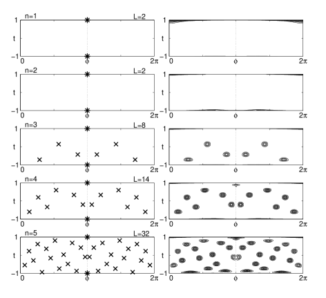
FIG. 3.: Comparison between the classical periodical orbits of length $n$ (crosses in the left column) and squared amplitude of quantum propagator $|\langle\theta,\varphi|(B_{S})^{n}|\theta,\varphi\rangle|^{2}$ (right column) for the baker map on the sphere. There exist $L$ periodic points of $(B_{S})^{n}$ (crosses). Two of them are localized on the north and south poles, and are symbolically represented by stars arbitrarily drawn at $\phi=\pi$.

Analysis of eigenvectors $|v_{i}\rangle$ of the quantum map $B_{S}$ provides an additional support for the quantum–classical correspondence. Generalized Husimi distribution of some eigenvectors, $H_{v_{i}}(\theta,\varphi)=|\langle v_{i}|\theta,\varphi\rangle|^{2}$, reveals maxima in the vicinity of some classical periodic orbits. This effect, called quantum scars [43], was already observed for the standard baker map on the torus[16].

The correspondence between a given classical system $M:X\to X$ and a family of quantum system $U_{j}:{\cal{H}}\to{\cal{H}}$, parametrized by the quantum number $j$, may be quantitatively characterized by the following condition of regular quantization. Let $C[(\theta,\varphi),\rho]$ denote the circle on the sphere of radius (angle) $\rho$ centered at $(\theta,\varphi)$. Let us define the quantity

$$I_{\rho}(\theta,\varphi):={2j+1\over 4\pi}\int_{C[M(\theta,\varphi),\rho]}|\langle\theta^{\prime},\varphi^{\prime}|U_{j}|\theta,\varphi\rangle|^{2}\sin\theta^{\prime}d\theta^{\prime}d\varphi^{\prime}$$ (21)

measuring localization of the Husimi function of the transformed state $U_{j}|\theta,\varphi\rangle$ in the $\rho$–neighborhood of the classical image $M(\theta,\varphi)$. Due to the normalization factor $(2j+1)/4\pi$ the integral of the Husimi function over the entire sphere $X$ is equal to one. If for any $\rho>0$

$$\lim_{N\to\infty}~{}~{}\inf_{(\theta,\varphi)}~{}\bigl{[}I_{\rho}(\theta,\varphi)\bigr{]}\to 1,$$ (22)

the quantization procedure linking the classical map $M$ and the family of quantum maps $U_{j}$ is called regular with respect to $SU(2)$ coherent states [44, 45]. The infimum is taken over all points $(\theta,\varphi)$ of the classical phase space, and the size of the Hilbert space $N=2j+1$ serves as a parameter in the family of quantum maps $U_{j}$.

Not being able to prove this condition analytically, we took for $M$ and $U$ the classical (16) and the quantum (14) baker maps on the sphere, respectively, and performed extensive numerical tests studying the dependence of $I_{\rho}$ on $N$ and $\rho$. Figure 4 shows how the quantity $I_{\rho}$ tends to unity in the semiclassical regime of large $N$. The mean value of $I_{\rho}$, averaged over $100$ points on the sphere, is close to unity at $N=600$ $(\circ)$, but the minimal value converges much slower $(\times)$. In spite of this fact, the above results confirm the existence of a tight relation between the classical and the quantum models of the baker map on the sphere, introduced in this paper.

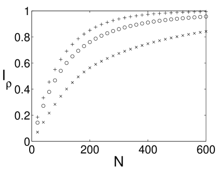
FIG. 4.: Regular quantization condition linking the classical (16) and the quantum (14) baker maps on the sphere. Dependence of the locally integrated Husimi functions $I_{\rho}$ on the size of the matrix $N$ for $\rho=\pi/15$. Symbol $(\circ)$ represents the mean value averaged over $100$ points placed uniformly on the sphere, while the maximal and the minimal values are denoted by $(+)$ and $(\times)$, respectively.

IV Statistical properties of the quantum map

Quantum maps corresponding to classically chaotic systems are expected to display the spectral fluctuations characteristic of random matrices [46, 47]. Due to the lack of the time reversal symmetry for the baker map on the sphere, unitary matrices $B_{S}$ should be compared to the Dyson’s circular unitary ensemble (CUE) [48, 49]. To obtain a satisfactory statistics we accumulated data from all four versions of the model (see appendix A) and several sizes of matrices.

Eigenphases $\phi_{l}$ of random unitary matrices are distributed uniformly in $[0,2\pi]$, so no unfolding of the spectrum is necessary. We numerically diagonalized matrices $B_{S}$, ordered the eigenphases and computed the rescaled spacings $s_{l}=(\phi_{l+1}-\phi_{l})/\langle s\rangle$, where $l=1,\dots,N-1$ and the mean spacing $\langle s\rangle$ is equal to $2\pi/N$. Figure 5 presents the near neighbors distribution $P(s)$ calculated from matrices $B_{S}$ with dimensions ranging from $N=50$ to $N=800$. The dashed line is the Wigner distribution $P_{u}(s)=32\pi^{-2}s^{2}\exp(-4s^{2}/\pi^{2})$ (exact for $2\times 2$ Hermitian matrices of the Gaussian unitary ensemble), which provides a very good approximation for the asymptotic CUE result obtained for $N\to\infty$ [47]. Collecting more data out of all four variants of the map we observed that the precision of the Wigner surmise is not satisfactory any more. Numerical data conform well to the exact CUE result, implemented as a power series [50], and shown in the inset. Note that for the unitary ensemble the differences between the Wigner surmise $P_{u}(s)$ and $P_{CUE}(s)$ do not exceed $5$ parts per thousand.

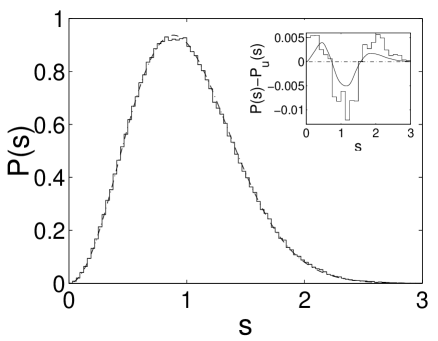
FIG. 5.: Eigenphases spacing statistics for quantum baker map on the sphere. Histogram contains 79524 data obtained for $N=50,\ldots,800$. Dashed line represents the Wigner distribution $P_{u}(s)$. Histogram in the inset consists of 318096 data and exhibits the difference from the Wigner surmise $P(s)-P_{u}(s)$. The solid line represents exact results for random matrices $P_{CUE}(s)-P_{u}(s)$.

To analyze the long range correlations we computed the spectral rigidity $\Delta_{3}$, introduced by Mehta and Dyson [51]. Numerical data obtained from matrices with dimensions $N=400\ldots 500$ are compared on Fig. 6 with CUE results represented by a dashed line. In addition we verified that the statistics of eigenvectors of matrices $B_{S}$ fit for large $N$ to the ${\chi^{2}}_{2}$ distribution predicted for CUE [47].

Since the matrix $B_{S}$ is orthogonal and its spectrum consists of two replicas of the same sequence, only the first $N/2$ spacings out of each matrix diagonalized were used in the statistics. Although the joint probability of eigenphases for random orthogonal matrices differs from this characteristic of CUE [52], the level spacing distribution are the same in the limit of large matrices. This fact, observed numerically [53], can be proved in a rigorous way [54]. Therefore it is not surprising that the orthogonal matrices representing the quantum baker map on the sphere exhibit CUE – like spectra.

Using $SU(2)$ coherent states it is possible to visualize the propagation of a wave packet. As before we use Husimi phase space representation. Fig. 7 presents contours of Husimi functions $H_{\Phi}$ with $\Phi=(B_{S})^{n}|\theta_{0},\varphi_{0}\rangle$ drawn in the ($t,\varphi$) coordinates. In other words each graph represents the subsequent iterate of the coherent state initially localized at $(\theta_{0},\varphi_{0})$. After each step the wave packet is squeezed along the $\varphi$-direction and stretched along the $t$-direction as predict the formula (16). At $n=4$ the state occupies the northern and the southern hemispheres so it is split into two part after the next iteration. Dimension of the Hilbert space $N$ is $200$. Observe an abrupt change in the shape of the wave packet occurring after $7-8$ iterations. This number corresponds well to the logarithmic time scale $n^{\star}=\log_{2}\,N\approx 7.6$, which determines the behavior of the quantum baker map on the torus [16] and often emerges in several problems of quantum chaos (see e.g. [55]). The same time scale $n^{\star}$ was observed for all other cases investigated ($N=10,24,50,100$).

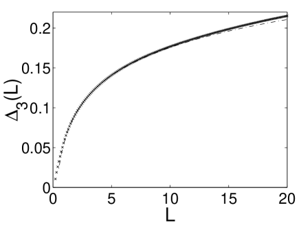
FIG. 6.: Spectral rigidity for the quantum baker map on the sphere. Crosses denote numerical data while the line represents the theoretical prediction for CUE.

Let us also mention that a generalized version of the model, discussed in Appendix C, covers also a system enjoying the time reversal symmetry. In this case, obtained for the parameter $\gamma$ set to $\pi/2$, the spectral statistics of the Floquet operators coincide with the predictions of the circular orthogonal ensemble (COE).

V Concluding remarks

In this paper we introduced classical and quantum versions of the baker map on the sphere. While the classical dynamics takes place on the sphere indeed, the name quantum baker map on the sphere cannot be treated literally: the quantum dynamics takes place in a finite dimensional Hilbert space $\cal{H}$, and a link with the classical dynamics on the sphere can be achieved with help of the $SU(2)$ coherent states. Nevertheless, our quantum model differs, in many respects, from the quantized baker maps of Balazs and Voros [15] and Saraceno [16]. In a specific case of the model it is represented by orthogonal matrices, which exhibit CUE – like statistical properties of the spectra. This fact reflects the lack of any antiunitary symmetry in this system. Since a time reversal case of the model, displaying a COE - like spectra, was found, the model proposed may be used to study the effects of the breaking of a generalized antiunitary symmetry.

Our construction is based on the properties of the Wigner matrix, representing rotation by the angle $\pi/2$. For each value of the classical parameter $\gamma$ we found four different families of quantum systems, parametrized by the even size $N$ the Hilbert space, which in the limit $N\to\infty$ seem to correspond to the same classical system. The condition of regular quantization with respect of $SU(2)$ coherent states has been checked to a satisfactory precision.

In the simplest case of the model ($\gamma=0$), the quantum baker map on the sphere is represented by real matrices. Thus the imaginary part of their traces vanish, in contrast to the quantum maps on the torus which suffer a logarithmical divergence of the imaginary part of the trace in the semiclassical limit [25].

If Fourier matrices are used in our construction in place of the Wigner rotation matrices, we obtain four versions of the quantized baker map on the torus, some of them different than these previously known. We hope that the new dynamical systems will prove their usefulness in further studies on the quantum – classical correspondence for chaotic systems.

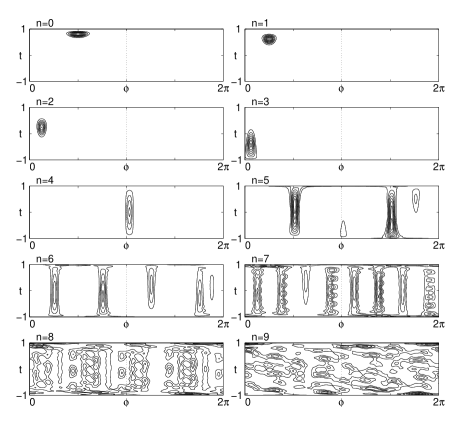
FIG. 7.: Evolution of the coherent state localized at $(\frac{1}{5}\pi,\frac{1}{2}\pi)$ under action of the baker map $B_{S}$ for $N=200$. Contours of Husimi function are plotted in the ($t,\varphi$) coordinates. Note the delocalization of the wave function for $n>\log_{2}200\approx 7.6$ iteration.

A Rotation matrix $R$ and unitarity of $R^{\prime}$

Components of the $N$ dimensional Wigner rotation matrix $R$, describing rotation around $y$-axes by the angle $\pi/2$, can be written as [35]

$$R_{k,m}=2^{-j}\sqrt{(j+m)!(j-m)!(j+k)!(j-k)!}\ S_{k,m}\ ,$$ (A1)

where $N=2j+1$ is even and $k,m=-j,-j+1,\dots,j-1,j$. The matrix $S_{k,m}$ reads

$$S_{k,m}=\sum_{p=\max(0,k-m)}^{\min(j+k,j-m)}\ \frac{(-1)^{p+m-k}}{p!\,(p+m-k)!\,(j-m-p)!\,(j+k-p)!}\ .$$ (A2)

We want to show the following identity

$$R_{-k,m}=(-1)^{j-m}R_{k,m}\ .$$ (A3)

To this end we start computing $R_{-k,m}$

$$R_{-k,m}=2^{-j}\sqrt{(j+m)!(j-m)!(j-k)!(j+k)!}\ S_{-k,m}\ .$$ (A4)

Rearranging the sum we get

$$S_{-k,m}=\sum_{p=\max(0,-k-m)}^{\min(j-k,j-m)}\ \frac{(-1)^{p+m+k}}{p!\,(p+m+k)!\,(j-m-p)!\,(j-k-p)!}\ .$$ (A5)

In (A5) we replace $p$ by $q=j-m-p$ (so $p=j-m-q$) and determine the new limits of summation: $q_{\min}=j-m-p_{\max}=-m-\min(-k,-m)=\max(0,k-m)$, while $q_{\max}=j-m-p_{\min}=j-m+\min(0,k+m)=\min(j+k,j-m)$. Now we rewrite the sum (A5)

$$S_{-k,m}=\sum_{q=\max(0,k-m)}^{\min(j+k,j-m)}\ \frac{(-1)^{j-m-q+m-k}}{(j-m-q)!\,(j+k-q)!\,q!\,(q+m-k)!}\ .$$ (A6)

Comparing the result with (A2) we can notice that

$$S_{-k,m}=(-1)^{j-m}S_{k,m}\,$$ (A7)

and the identity (A3) follows.

Unitarity of the $N/2\times N/2$ matrix $R^{\prime}$ will be deduced from the unitarity of $R$

$$\sum_{k=-j}^{j}R^{\dagger}_{\ l,k}R_{k,m}=\sum_{k=-j}^{j}R_{k,l}R_{k,m}=\delta_{l,m}\ .$$ (A8)

This sum may be divided into two parts

$$\sum_{k=-j}^{-\frac{1}{2}}\left(R_{k,l}R_{k,m}+R_{-k,l}R_{-k,m}\right)=\delta_{l,m}\ .$$ (A9)

Now we use property (A3) to reformulate the first part of the sum

$$\sum_{k=-j}^{-\frac{1}{2}}R_{k,l}R_{k,m}\left(1+(-1)^{2j-l-m}\right)=\delta_{l,m}\ .$$ (A10)

Choosing odd columns of matrix $R$ reduces to exchange $l\rightarrow 2l+j$, and $m\rightarrow 2m+j$, so $2j-l-m\rightarrow-2(l+m)$. Since $N$ is even, $j$ and the indices $l$ and $m$ are half integer, so $l+m$ is an integer number. We can rewrite the result

$$2\sum_{k=-j}^{-\frac{1}{2}}R_{k,2l+j}R_{k,2m+j}=\delta_{2l+j,2m+j}=\delta_{l,m}\ .$$ (A11)

This proves that choosing upper halves of even columns of the matrix $\sqrt{2}R$ gives an unitary $N/2\times N/2$ matrix $R^{\prime}$. Choosing odd columns or bottom halves ($k>0$) gives other unitary matrices of the size $N/2$.

B Four versions of quantum baker map on the sphere

As shown in appendix A the auxiliary matrices $R^{\prime}$ and $R^{\prime\prime}$ are unitary, and can be constructed out of the elements of the rotation matrix $R$ in several ways. Let us introduce the indices $a,b=0,1$ denoting, whether the odd or the even columns of $R$ where used in the construction. This allows us to define four unitary matrices

$${R^{\prime}}_{k,l}^{(a)}:=\sqrt{2}R_{k,2l+j+a},\ \ k,l=-j\ldots-\frac{1}{2};\ \ {R^{\prime\prime}}_{k,l}^{(b)}:=\sqrt{2}R_{k,2l-j-1+b},\ \ k,l=\frac{1}{2}\ldots j;$$ (B1)

which lead to four different variants of the quantum baker map on the sphere for each even $N$

$${B_{S}}^{(ab)}=R^{-1}\left[\begin{array}[]{cc}R^{\prime(a)}&0\\ 0&R^{\prime\prime(b)}\end{array}\right]$$ (B2)

with $a,b=0,1$. Each of matrices ${B_{S}}^{(ab)}$ is orthogonal and my be generalized into a one parameter family of unitary matrices according to formula (15). For concreteness we provide here some examples. For $N=2$ any unitary matrix is equivalent to rotation, and formula (B2) gives

$\displaystyle{B_{S}}^{(00)}={B_{S}}^{(10)}=\frac{1}{\sqrt{2}}\left[\begin{array}[]{cc}1&1\\ 1&-1\end{array}\right]\ \ \ {\rm{and}}\ \ {B_{S}}^{(01)}={B_{S}}^{(11)}=\frac{1}{\sqrt{2}}\left[\begin{array}[]{cc}1&-1\\ 1&1\end{array}\right].$

Simplest interesting matrices appear for $N=4$

$\displaystyle{B_{S}}^{(00)}=\frac{1}{\sqrt{8}}\left[\begin{array}[]{cccc}2&0&2&0\\ \sqrt{3}&1&-\sqrt{3}&-1\\ 0&2&0&2\\ -1&\sqrt{3}&1&-\sqrt{3}\end{array}\right],\ \ {B_{S}}^{(01)}=\frac{1}{\sqrt{8}}\left[\begin{array}[]{cccc}2&0&-\sqrt{3}&1\\ \sqrt{3}&1&2&0\\ 0&2&-1&-\sqrt{3}\\ -1&\sqrt{3}&0&2\end{array}\right],$

$\displaystyle{B_{S}}^{(10)}=\frac{1}{\sqrt{8}}\left[\begin{array}[]{cccc}\sqrt{3}&-1&2&0\\ 2&0&-\sqrt{3}&-1\\ 1&\sqrt{3}&0&2\\ 0&2&1&-\sqrt{3}\end{array}\right],\ \ {B_{S}}^{(11)}=\frac{1}{\sqrt{8}}\left[\begin{array}[]{cccc}\sqrt{3}&-1&-\sqrt{3}&1\\ 2&0&2&0\\ 1&\sqrt{3}&-1&-\sqrt{3}\\ 0&2&0&2\end{array}\right].$

Observe that the first $N/2$ columns of ${B_{S}}^{(00)}$ and ${B_{S}}^{(01)}$ are equal, while the same is true for ${B_{S}}^{(11)}$ and ${B_{S}}^{(10)}$. Moreover, the matrices ${B_{S}}^{(00)}$ and ${B_{S}}^{(10)}$ share the same last $N/2$ columns; the same is true for ${B_{S}}^{(01)}$ and ${B_{S}}^{(11)}$. These relations, valid for arbitrary even $N$, follow directly from the definition (B2). To emphasize the differences between all four variants of the quantum system let us consider the trace of each matrix. It is easy to show that for any $N$ the matrices ${B_{S}}^{(10)}$ are traceless: Tr${B_{S}}^{(10)}=0$. Moreover, Tr${B_{S}}^{(01)}=\sqrt{2}$, while Tr${B_{S}}^{(00)}+$Tr${B_{S}}^{(11)}=\sqrt{2}$. For $N=6$ the traceless baker map is represented by the matrix

$\displaystyle{B_{S}}^{(10)}=\frac{1}{8\sqrt{2}}\left[\begin{array}[]{cccccc}3\sqrt{5}&-{\sqrt{10}}&3&8&0&0\\ 8&0&0&-3\sqrt{5}&-3\sqrt{2}&1\\ 3\sqrt{2}&6&-{\sqrt{10}}&0&8&0\\ 0&8&0&\sqrt{10}&-6&-3\sqrt{2}\\ -1&3\sqrt{2}&3\sqrt{5}&0&0&8\\ 0&0&8&-3&\sqrt{10}&-3\sqrt{5}\end{array}\right].$

C A family of systems parametrized by a classical parameter $\gamma$

Discussed quantum system may be generalized by picking for $R$ a different rotation matrix. Let us allow for a rotation along an arbitrary axis, which belongs to the the plane $xy$ and forms the angle $\gamma$ with the $y$-axis. The transformation matrix from the $|m\rangle_{z}$ basis to the new basis takes the form

$${R^{\gamma}}_{m^{\prime},m}={}_{z}\langle m|e^{i\gamma J_{z}}e^{-i\frac{\pi}{2}J_{y}}e^{-i\gamma J_{z}}|m^{\prime}\rangle_{z}\ .$$ (C1)

Replacing the rotation matrix $R$ by $R^{\gamma}$ in the formulae (B1) and (B2) we obtain a continuous family of quantum models $B_{\gamma}^{(ab)}$ parameterized by the angle $\gamma\in[0,2\pi)$ and corresponding to a various directions of squeezing.

We can find the classical counterpart of the generalized quantum model

$$\left(t^{\prime},\varphi^{\prime}\right)=\left\{\begin{array}[]{ll}\left(2t-1,\left\{\left[(\varphi+\pi+2\gamma)\mbox{ mod }2\pi\right]/2+\frac{3}{2}\pi+\gamma\right\}\mbox{ mod }2\pi\right)&\mbox{for $t\geq 0$}\\ \left(2t+1,\left\{\left[(\varphi+\pi+2\gamma)\mbox{ mod }2\pi\right]/2+\frac{1}{2}\pi+\gamma\right\}\mbox{ mod }2\pi\right)&\mbox{for $t<0$}\end{array}\right..$$ (C2)

This reduces to (16) for $\gamma=0$. Figure 8 shows how the sphere is mapped onto itself by the formula (C2). The sphere is cut along meridian ($\varphi=\pi+2\gamma$). The northern and the southern hemispheres are stretched in the $t$-direction by the factor of $2$ and are squeezed in the $\varphi$-direction. The transformed blocks are respectively placed on the east and on the west from the meridian ($\varphi=\pi/2+\gamma$).

FIG. 8.: Generalized classical baker map on the sphere drawn in the ($t,\varphi$) coordinates for $\gamma=\pi/6$. The parts $A_{1}$, $A_{2}$, $B_{1}$, $B_{2}$ are linearly transformed into $A^{\prime}_{1}$, $A^{\prime}_{2}$, $B^{\prime}_{1}$, $B^{\prime}_{2}$.

For $\gamma=\pi/2$ the matrix $R^{\gamma}$ describes the rotation by $\pi/2$ around the $x$-axis. In this case the classical map is symmetric with respect to the reflection along the $x$-axis and has a generalized time reversal symmetry. Existence of the geometric symmetry corresponds in the quantum case to the fact that the Floquet operator $B_{\pi/2}^{(ab)}$ commutes with the reflection matrix $V_{nn^{\prime}}=\delta_{n,N-1-n^{\prime}}$. Therefore one can divide its eigenstates into two classes: the symmetric and the antisymmetric states. Analyzing the spectral statistics separately in both parity classes we find the COE-like behavior of the spectrum. By varying the classical angle $\gamma$ in the vicinity of $\pi/2$ one may study the influence of the time reversal symmetry and the geometric symmetry on the system.

D Four versions of quantum baker map on the torus

In this appendix we obtain four variants of the baker map on the torus and show their relation to the earlier models [15, 16]. Consider the generalized Fourier matrix [25] which is the transformation matrix from position $q$ to momentum $p$ basis on the torus

$$\left[{F_{N}}^{\chi_{q}\chi_{p}}\right]_{k,l}=\frac{1}{\sqrt{N}}\ e^{-2\pi i(k+\chi_{q})(l+\chi_{p})/N}.$$ (D1)

The phases $\chi_{q},\chi_{p}\in[0,1)$ may be treated as free parameters, which correspond to the phases gained by the wave function after translation by one period in the $q$ and in the $p$ direction, respectively. The matrix ${F_{N}}^{\chi_{q}\chi_{p}}$ is unitary. Assuming that the matrix size $N$ is even, we may apply the procedure of taking every second half of column to obtain four auxiliary matrices of size $N/2$

$$\left[{F^{\prime}_{N/2}}^{\chi_{q}\chi_{p}\,(a)}\right]_{k,l}:=\sqrt{2}\left[{F_{N}}^{\chi_{q}\chi_{p}}\right]_{k,2l+a}\ ;\ \ \left[{F^{\prime\prime}_{N/2}}^{\chi_{q}\chi_{p}\,(b)}\right]_{k,l}:=\sqrt{2}\left[{F_{N}}^{\chi_{q}\chi_{p}}\right]_{k+N/2,2l+b}$$ (D2)

where $a,b=0,1$, and the indices run $k,l=0,\ldots,N/2-1$. Both matrices $F^{\prime\,(a)}$ are unitary, since

$\displaystyle\sum_{l=0}^{N/2-1}\ \frac{2}{N}\ e^{-2\pi i(k+\chi_{q})(2l+a+\chi_{p})/N}\,e^{2\pi i(k^{\prime}+\chi_{q})(2l+a+\chi_{p})/N}=\sum_{l=0}^{N/2-1}\ \frac{2}{N}\ e^{2\pi i(k^{\prime}-k)(2l+a+\chi_{p})/N}=$

$\displaystyle=e^{2\pi i(k^{\prime}-k)(a+\chi_{p})/N}\sum_{l=0}^{N/2-1}\ \frac{1}{N/2}\ e^{2\pi i(k^{\prime}-k)l/(N/2)}=\delta_{k,k^{\prime}}\ ,$

and the same holds for both matrices $F^{\prime\prime\,(b)}$. Hence the four versions of quantum baker map on the torus take the familiar form

$${B_{T}}^{\chi_{q}\chi_{p}\,(ab)}:=\left[{F_{N}}^{\chi_{q}\chi_{p}}\right]^{-1}\left[\begin{array}[]{cc}{F^{\prime}_{N/2}}^{\chi_{q}\chi_{p}\,(a)}&0\\ 0&{F^{\prime\prime}_{N/2}}^{\chi_{q}\chi_{p}\,(b)}\end{array}\right].$$ (D3)

The matrix ${B_{T}}^{00\,(00)}$ is equivalent to the original quantum baker map of Balazs and Voros [15], while the symmetric map of Saraceno [16] is defined as follows

$$B:=\left[{F_{N}}^{1/2,1/2}\right]^{-1}\left[\begin{array}[]{cc}{F_{N/2}}^{1/2,1/2}&0\\ 0&{F_{N/2}}^{1/2,1/2}\end{array}\right].$$ (D4)

Two versions of our map ${B_{T}}^{1/2,1/2\,(10)}$, ${B_{T}}^{1/2,1/2\,(01)}$ are also symmetric in respect to reflection ($VB_{T}V^{-1}=B_{T}$ where $V_{n,n^{\prime}}=\delta_{n,N-1-n^{\prime}}$), as the map of Saraceno. The real part of their traces do not change with $N$ and is equal to $0$ and $\sqrt{2}$, respectively. They correspond to the same classical baker map on the torus and might be useful for further semiclassical investigation of this model.

Statistical analysis of spectra of these two variants ${B_{T}}^{1/2,1/2\,(01)}$, ${B_{T}}^{1/2,1/2\,(10)}$ of several dimension $N\in[50,600]$ shows that the level spacing distribution $P(s)$ conforms to predictions of circular orthogonal ensemble with a precision allowing one to discriminate the Wigner surmise. The same was checked for the matrix of Saraceno. Due to symmetry of the problem the statistical data were collected separately in each parity class containing $N/2$ eigenvalues.

REFERENCES

- [1] Arnold V I and Avrez A 1965 Ergodic Problems of Classical Mechanics (New York: Benjamin)
- [2] Reichl L E 1992 The Transition to Chaos: In Conservative Classical Systems: Quantum Manifestations (New York: Springer-Verlag)
- [3] Ott E 1993 Chaos in Dynamical Systems (New York: Cambridge University Press)
- [4] Farmer J D, Ott E and Yorke J A 1983 Physica 7D 153
- [5] Alexander J C and Yorke J A 1984 Ergod. Th. Dynam. Sys. 4 1
- [6] Romeiras F J, Greborgi C and Ott E, 1990 Phys. Rev. A 41 784
- [7] Namenson A, Ott E and Antonsen T M 1996 Phys. Rev. E 53 2287
- [8] Gaspard P 1992 J. Stat. Phys 68 673
- [9] Vollmer J, Tel T and Breymann W 1997 Phys. Rev. Lett. 79 2759
- [10] Antoniou I and Tasaki S 1992 Physica A 190 303
- [11] Hasegawa H H and Sapir W C 1992 Phys. Rev. A 46 7401
- [12] Gaspard P 1993 Chaos 3 427
- [13] Hasegawa H H and Driebe D J 1994 Phys. Rev. E 50 1781
- [14] Fox R F 1997 Chaos 7 254
- [15] Balazs N L and Voros A 1989 Ann. Phys. 190 1
- [16] Saraceno M 1990 Ann. Phys. 199 37
- [17] De Bièvre S, Degli Esposti M and Giachetti R 1996 Com. Math. Phys. 176 73
- [18] Rubin R and Salwen N 1998 preprint Los Alamos quant-ph/9807045
- [19] Ozorio de Almeida A M and Saraceno M 1991 Ann. Phys. 210 1
- [20] O’Connor P W and Tomsovic S 1991 Ann. Phys. NY 207 218
- [21] Saraceno M and Voros A 1992 Chaos 2 99
- [22] O’Connor P W, Tomsovic S and Heller E J 1992 J. Stat. Phys. 68 131
- [23] O’Connor P W, Tomsovic S and Heller E J 1992 Physica D 55 340
- [24] Lakshminarayan A and Balazs N L 1993 Ann. Phys. 226 350
- [25] Saraceno M and Voros A 1994 Physica D 79 206
- [26] Eckhardt B and Haake F 1994 J. Phys. A 27 4449
- [27] Lakshminarayan A 1995 Ann. Phys. 239 272
- [28] Toscano F, Vallejos R O and Saraceno M 1997 Nonlinearity 10 965
- [29] Kaplan L and Heller E J 1998 preprint Los Alamos chao-dyn/9809008
- [30] Gutzwiller M C 1971 J. Math. Phys. 12 343
- [31] Gutzwiller M C 1990 Chaos in Classical and Quantum Mechanics (Berlin: Springer-Verlag)
- [32] Schack R and Caves C M 1993 Phys. Rev. Lett. 71 525
- [33] Hannay J H, Keating J P and Ozorio de Almeida A M 1994 Nonlinearity 7 1327
- [34] Schack R 1998 Phys. Rev. A 57 1634
- [35] Rose M E 1957 Elementary theory of angular momentum (London: John Wiley and sons inc., New York: Chapman and Hall Ltd.)
- [36] Rényi A 1970 Probability Theory (Budapest: Akadémiai Kiadó)
- [37] Pakoński P to be published
- [38] Radcliffe J M 1971 J. Phys. A: Gen. Phys. 4 313
- [39] Arecchi F T, Courtens E, Gilmore R and Thomas H 1972 Phys. Rev. A 6 2211
- [40] Perelomov A 1986 Generalized Coherent States and Their Applications (Berlin: Springer-Verlag)
- [41] Hecht K T 1987 The Vector Coherent State Method and Its Application to Problems of Higher Symmetries (Berlin: Springer-Verlag)
- [42] Vieira V R and Sacramento P D 1995 Ann. Phys. NY 242 188
- [43] Heller E J 1984 Phys. Rev. Lett. 53 1515
- [44] Kifer Y 1988 Random Perturbations of Dynamical Systems (Boston: Birkhäuser)
- [45] Słomczyński W and Życzkowski K 1994 J. Math. Phys. 35 5674
- [46] Bohigas O 1991 Chaos and Quantum Physics (Les Houches Summer School) ed M J Giannoni, A Voros and J Zinn-Justin (Amsterdam: North-Holland) Session LII
- [47] Haake F 1991 Quantum Signatures of Chaos (Berlin: Springer-Verlag)
- [48] Dyson F J 1962 J. Math. Phys. 3 140, 157, 166
- [49] Mehta M L 1991 Random Matrices 2 ed. (New York: Academic Press)
- [50] Dietz B and Haake F 1990 Z. Phys. B 80 153
- [51] Dyson F J and Mehta M L 1963 J. Math. Phys. 4 701
- [52] Girko V L 1990 Theory of Random Determinants (Kluwer: Dordrecht)
- [53] Poźniak M, Życzkowski K and Kuś M 1998 J. Phys. A 31 1059
- [54] Sarnak P private communication
- [55] Casati G and Chirikov B (eds.) 1995 Quantum Chaos. Between Order and Disorder (Cambridge: Cambridge University Press)