Globally coupled maps with asynchronous updating

Abstract

We analyze a system of globally coupled logistic maps with asynchronous updating. We show that its dynamics differs considerably from that of the synchronous case. For growing values of the coupling intensity, an inverse bifurcation cascade replaces the structure of clusters and ordering in the phase diagram. We present numerical simulations and an analytical description based on an effective single-element dynamics affected by internal fluctuations. Both of them show how global coupling is able to suppress the complexity of the single-element evolution. We find that, in contrast to systems with synchronous update, internal fluctuations satisfy the law of large numbers.

]

I Introduction

Introduced by Kaneko in 1984 [1], coupled map lattices have proved to be a powerful tool in the study of spatiotemporal chaos and pattern formation in complex systems [2, 3, 4, 5, 6, 7]. They have found applications as models in different branches of science [8, 9, 10, 11]. Globally coupled maps [3], which bear similarity to the Sherrington-Kirkpatrick model, constitute a kind of mean-field extension of coupled map lattices. In an ensemble of globally coupled maps, the elements are seen to form clusters of synchronized activity. As the coupling increases, a variety of phases can be identified—from coherent, through ordered and partially ordered, to turbulent—depending on the number of clusters in the system. For sufficiently large coupling intensities, the generic behavior consists of full synchronization of the whole population, with all the elements having identical evolution.

In usual models of globally coupled maps the elements update their state at the same time, namely, their evolution is synchronous. For an ensemble of $N$ elements whose individual dynamics is given by the nonlinear map $x_{i}(t+1)=f[x_{i}(t)]$, a typical scheme for global coupling is given by

$$x_{i}(t+1)=(1-\epsilon)f[x_{i}(t)]+\frac{\epsilon}{N}\sum_{j=1}^{N}f[x_{j}(t)],\ i=1,\dots,N,$$ (1)

where $\epsilon\in[0,1]$ is the coupling intensity. Equation (1) is applied synchronously to all the maps of the system, with the values of all the sites at the previous time as inputs.

From a realistic viewpoint, however, synchronous updating does not seem to be very plausible in models of real systems [12, 13, 14, 15]. As discussed, for instance, for neural networks [16], an independent choice of the times at which the elements of a given complex system update their respective states should provide a closer approximation to reality. It has however to be mentioned that, in systems with local coupling, asynchronous update has been shown to lead to trivial behavior [6]. We present here a first analysis of asynchronous globally coupled maps and find their behavior to be completely different from that of the usual synchronous models. We have analyzed two possible asynchronous schemes:

  (a)

At each time step, update the elements according to the sequence given by a prescribed “list” that contains every element once. The order of the elements in the list is chosen at random at each step.

  (b)

Divide each time step into $N$ substeps. At each substep, update one element chosen at random. After $N$ substeps the map operates, on average, once over each element in the system.

For the sake of clarity, let us formulate mathematically the second scheme. Let $\eta(t)$ be a stochastic process that takes an integer value $\eta=1,2,\dots,N$ at each substep, with uniform probability. The dynamics proceeds in the following way:

$$x_{i}(t+\frac{1}{N})=\left\{\begin{array}[]{ll}(1-\epsilon)f[x_{i}(t)]+{\displaystyle\frac{\epsilon}{N}\sum_{j}}f[x_{j}(t)]&\mbox{if $i=\eta(t)$,}\\ x_{i}(t)&\mbox{if $i\neq\eta(t)$.}\end{array}\right.$$ (2)

In the first scheme, $\eta(t)$ takes the values $1,2,...,N$ at random, but only once within each time step. It can be seen that, in this dynamics, the mean field $F(t)=N^{-1}\sum_{j}f[x_{j}(t)]$ has different values when acting over different elements, as time proceeds by steps of length $1/N$. This feature and the fact that asynchronous updating incorporates a stochastic component in the evolution, contrast with the deterministic synchronous scheme (1).

Evolution under the two asynchronous schemes introduced above displays the same global properties. However, in the second scheme one or more elements may fail to be updated in some time step. As a consequence, since $N$ updates have to be made during a time step, some other elements will be updated more than once. This has nontrivial consequences in the dynamics, to be discussed below. Besides, the second scheme has the advantage of being much faster computationally.

In this paper, we analyze an ensemble of globally coupled logistic maps. We show that the dynamics under asynchronous updating substantially differs from that of the synchronous case. The structure of clustered phases completely dissapears. In its place, an inverse bifurcation cascade develops as the coupling intensity is increased. In the following, we analyze this phenomenon from numerical simulations and construct a phase diagram for the different regimes displayed by the dynamics. Then, we propose an analytical explanation for the bifurcation cascade, whose results compare successfully with the numerical data. Finally, we discuss how the fluctuations generated in the internal dynamics are reflected in the average evolution.

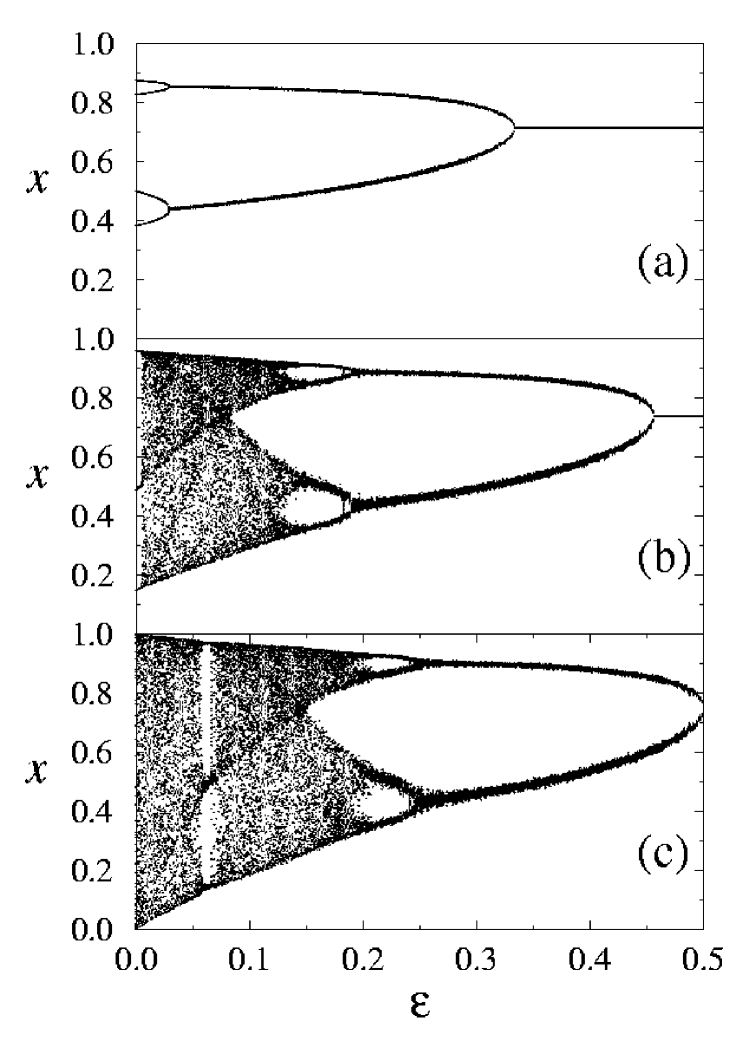
FIG. 1.: Bifurcation diagrams of a system of $N=1000$ logistic maps, as a function of the coupling intensity $\epsilon$. The diagrams are constructed following the evolution of a single element taken at random, with (a) $\lambda=3.5$, (b) $\lambda=3.84$, (c) $\lambda=4$.

II Inverse bifurcation cascade and phase diagram

In this section we present extensive numerical simulations of the evolution given in Eq. (2) for the standard logistic map, $f(x)=\lambda x(1-x)$. We concentrate in the values of $\lambda$ where this map displays its bifurcation cascade, $3<\lambda<4$, leading through period doubling from a stable fixed-point state to a completely developed chaotic regime. For reasons that will become evident later, we restrict the coupling intensity $\epsilon$ to the interval $0<\epsilon<0.5$.

In Fig. 1 we show the bifurcation diagrams for the evolution of a single element, chosen at random from a population of $10^{3}$ maps, as a function of $\epsilon$, for three values of $\lambda$. These diagrams are constructed as usual. For given values of $\epsilon$ and $\lambda$ the system is let to evolve until transients have elapsed. Then, the state of the chosen element is recorded and plotted at some successive time steps.

Figure 1(a) shows the bifurcation diagram for $\lambda=3.5$, where the (uncoupled) logistic map evolves in a period-4 orbit. As $\epsilon$ grows, the four initial branches collapse into two branches which, in turn, merge into a single branch. Increasing the coupling intensity leads thus the evolution of a single element to display an inverse bifurcation cascade. The same scenario occurs for other values of $\lambda$. For $\lambda=0.38$, where the logistic map is within its largest period-3 stability window, increasing $\epsilon$ leads the evolution to successively exhibit chaotic regimes of one and two bands and, eventually, stable branches that finally collapse into a single stable state (Fig. 1(b)). For $\lambda=4$, in the extreme chaotic regime of the logistic map, the full bifurcation diagram is run over backwards (Fig. 1(c)).

It is apparent from Fig. 1 that the evolution of a single element in the ensemble is subject to the action of noise. Indeed, the branches of nonchaotic evolution are not perfectly defined—except in the case of a single stable state—and high-order bifurcations, close to the onset of chaos, are clearly suppressed. This noise, which is produced internally in the system via the asynchronous updating, induces spreading of the states visited during the evolution when the coupling is different from zero.

The branches of nonchaotic evolution, with their small but noticeable dispersion, are what remains of the stable periodic orbits of the deterministic map under the effect of the internal noise. In these branches, the evolution driven by the two schemes presented in the Introduction differ. Scheme (a) defines true noisy periodic orbits, where each element visits the set of available states following the same periodic sequence as the deterministic map. On the contrary, scheme (b) allows some elements to skip the update in a time step. Consequently, some other elements are updated more than once. As a result, the observed successive states do not follow a periodic sequence. To simplify the discussion, in the following we will call these regimes of noisy nonchaotic (periodic or nonperiodic) evolution “period-$n$” orbits, referring rather to the set of states visited by each element.

The chaotic bands, meanwhile, are also blurred by the internal noise. We will thus refer to a regime where a noise-free map would exhibit deterministic chaotic evolution as an “$n$-band” chaotic region.

To summarize the variety of behavior observed for a single element as $\epsilon$ and $\lambda$ vary, we have constructed a phase diagram in the plane spanned by these two parameters for a population of $10^{3}$ elements. For each value of $\epsilon$ and $\lambda$ the evolution has been calculated with scheme (b) during $10^{4}$ time steps. After a transient of $5\times 10^{3}$ steps, a 500-column histogram over the states visited by a single element in the remaining $5\times 10^{3}$ steps has been produced to identify the kind of evolution corresponding to those values of the parameters. The phase diagram is shown in Fig. 2. Each region in this diagram corresponds to a different kind of attractor.

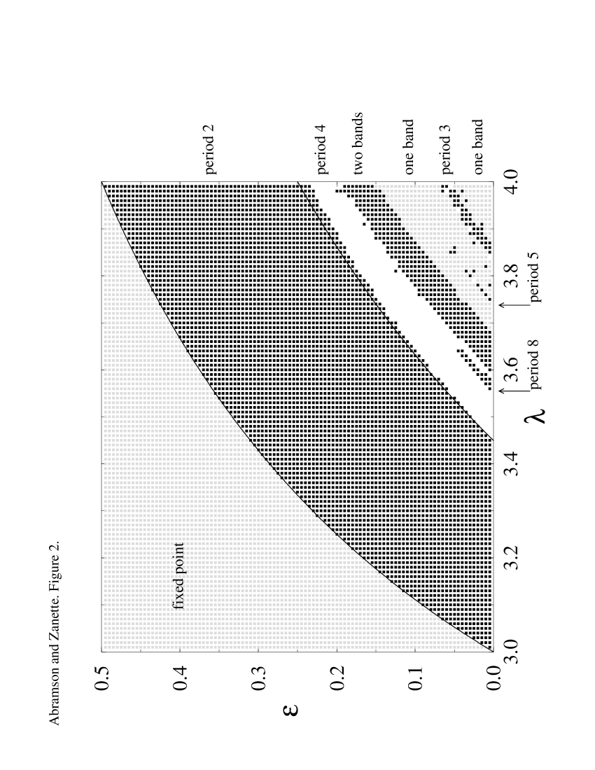
FIG. 2.: Phase diagram of a system of $N=1000$ logistic maps. The two lines are the analytic curves given by Eqs. (6) and (8).

The large upper-left region corresponds to a fixed point. In this zone of the parameter space, from any initial condition, all the elements are attracted to the same stable fixed point. Without coupling—i.e. for $\epsilon=0$, on the horizontal axis of the plot—such behavior would be observed for $\lambda<3$ only. At larger values of $\lambda$ and, notably, even up to the fully developed chaotic regime ($\lambda=4$), there always exists a coupling intensity able to suppress the complex behavior of the uncoupled system. As mentioned above, in this fixed-point regime internal noise is also suppressed.

Below the fixed-point region, there is a series of zones shown, alternately, with black squares and empty space in Fig. 2. In this phases the evolution of single elements display “periodic” and “chaotic” noisy orbits, as indicated in the plot. Due to the noise, the limits between these regions are not sharply defined and some of the zones—such as the period-8 and the period-5 regions—are truncated at certain values of $\lambda$ and $\epsilon$. Between the zones of period-4 orbits and two-band chaotic evolution, higher-order periodic orbits as well as chaotic evolution in more than two bands are missing. The period-3 stability window is instead clearly detected, immersed in the one-band chaotic regime.

Since blurring of boundaries between zones and suppression of higer-order periodic and chaotic orbits are a direct consequence of the internal noise, it is expected that—if noise decreases upon incresing the number of elements in the ensemble—the phase diagram becomes more sharply defined for higher $N$. It is however known that, in synchronous globally coupled maps, the internal noise does not decrease in the usual self-averaging way as $N^{-1/2}$—as predicted by the so-called law of large numbers—but in a much slower manner [17, 18]. In Section IV we analyze this aspect for asynchronous evolution, finding that the law of large numbers is recovered in these systems.

Note finally that if, in contrast with Fig. 1, the bifurcation diagram would be plotted for fixed $\epsilon$ as a function of $\lambda$, the bifurcation cascade would proceed forwards. For large values of the coupling intensity, however, higher-order bifurcations and chaos would not be reached even for $\lambda=4$.

III Mean field approach

It is possible to describe analytically some features of the bifurcation cascade by performing a kind of mean field approximation to Eq. (2). From the viewpoint of a single element, updating of its state occurs, in average, once per time step. At the successive times where a given element is updated, the sequence of values of the mean field $F(t)=N^{-1}\sum_{j}f[x_{j}(t)]$ fluctuates due to the evolution of the individual states of all the elements, effectively resembling a stochastic process. In such a way, the single-element dynamics can be though of as given by a deterministic map subject to the action of an effective “external” stochastic forcing.

In order to characterize this effective forcing, we assume—as suggested by the numerical simulations—that the evolution of the system (2) determines, at long times, a well-defined measure $\mu(x)$ on the space $x$. At any time step the value of the elements will distribute according to this measure and, for $N\to\infty$, the mean field $F(t)$ will approach a constant $F_{0}=\int f(x)\mu(x)dx$. For finite $N$, however, the field $F(t)$ will fluctuate around $F_{0}$, so that we can write

$$\lim_{t\to\infty}F(t)\approx F_{0}+\xi(t),$$ (3)

where $\xi(t)$ is a stochastic process of zero mean.

Within this approximation, the dynamics of a single element is

$$x_{i}(t+1)=(1-\epsilon)f[x_{i}(t)]+\epsilon F_{0}+\epsilon\xi(t),$$ (4)

The effective individual evolution is thus given by a deterministic renormalized map $f^{\rm eff}(x)=(1-\epsilon)f(x)+\epsilon F_{0}$ upon which an additive noisy force of zero mean acts. It has to be noticed that the constant $F_{0}$, being determined by the collective dynamics, prevents the population from complete decoupling.

It is well known that a deterministic map subject to the action of a moderate additive noise of zero mean preserves its critical behavior, the only effect of noise being the suppression of high-order bifurcations. Within this picture, we can then explicitely calculate the first bifurcation points as follows.

Suppose firstly that the map $f^{\rm eff}(x)$ has a stable fixed point $x_{0}$ as its only attractor. Since—in the absence of noise—all the elements are attracted to it, we have $\mu(x)=\delta(x-x_{0})$ and $F_{0}=f(x_{0})$. The effective single-element evolution becomes thus $x_{i}(t+1)=(1-\epsilon)f[x_{i}(t)]+\epsilon f(x_{0})$. The equation

$$x_{0}=(1-\epsilon)f(x_{0})+\epsilon f(x_{0})=f(x_{0}),$$ (5)

determines $x_{0}$, which results to coincide with the fixed point of the original map $f(x)$. The evolution equation can be now readily linearized to find that $x_{0}$ is stable if the coupling intensity satisfies

$$\epsilon>\epsilon_{c}^{1}=1-|f^{\prime}(x_{0})|^{-1}.$$ (6)

For the logistic map, that has a stable fixed point at $x_{0}=1-\lambda^{-1}$ for $1<\lambda<3$, Eq. (6) implies that the state $x_{i}=x_{0}$ is stable if $\epsilon>1-|2-\lambda|^{-1}$. That is, for $2<\lambda<3$ the state is stable for all $\epsilon$ and, for $\lambda>3$ it is stable for $\epsilon$ large enough. In Fig. 2 we have drawn the curve $\epsilon_{c}^{1}(\lambda)$ that defines the boundary between the fixed point and the period-2 regions. This analytical result is in full agreement with simulations.

A similar argument can be applied to period-2 orbits. Due to the randomness of the updating scheme, at each time step practically one half of the elements will be at one of the two states of the orbit, say $x_{A}$, and the other half at the other, $x_{B}$. The corresponding invariant measure is $\mu(x)=[\delta(x-x_{A})+\delta(x-x_{B})]/2$ and $F_{0}=[f(x_{A})+f(x_{B})]/2$. Therefore, the equations which determine the values of $x_{A}$ and $x_{B}$ are

$$\begin{array}[]{rcl}x_{A}&=&(1-\epsilon)f(x_{B})+\epsilon[f(x_{A})+f(x_{B})]/2\\ x_{B}&=&(1-\epsilon)f(x_{A})+\epsilon[f(x_{A})+f(x_{B})]/2.\end{array}$$ (7)

These equations are equivalent to $x_{A}=f(x_{B})$ and $x_{B}=f(x_{A})$, so that $F_{0}=(x_{A}+x_{B})/2$ and $x_{A,B}$ are also the two states corresponding to the period-2 orbit of the original map $f(x)$. For the logistic map these equations can be solved, and the stability condition implies

$$\epsilon>\epsilon_{c}^{2}=\frac{-1-2\lambda+\lambda^{2}-\sqrt{1-6\lambda+3\lambda^{2}}}{\lambda(\lambda-2)}.$$ (8)

The line $\epsilon_{c}^{2}(\lambda)$ is also shown in Fig. 2, separating the regions of period-2 and period-4 orbits. This result is again in good agreement with simulations, though a slight deviation is observed for large values of $\epsilon$, i.e. near $\lambda=4$. This deviation can be ascribed to the increasing effect of noise for growing $\epsilon$ (cf. Eq. (4)), that blurs the boundaries where bifurcations occur.

Analogous reasoning may be used to determine the boundaries between other zones. For higher-order periodic orbits, however, the equations cannot be explicitly solved in the case of the logistic map. For chaotic evolution, moreover, the measure $\mu(x)$ should be obtained numerically.

IV Fluctuations of the mean field

A key ingredient in the analysis presented in the previous section is the assumption that, for large populations, the system (2) defines a measure in the one-element state space $x$, such that for sufficiently long times the elements exhibit a well-defined distribution in $x$. It is implicit in that assumption that the amplitude of internal noise decreases as $N$ grows. As mentioned above, however, previous work has shown that fluctuations in deterministic synchronous globally coupled systems does not self-average in the usual way [17, 18]. It is therefore worthwhile to analyze this point in some detail for the present case of asynchronous update.

The fluctuating part of the mean field, $\xi(t)$ in Eq. (3), can also be analytically studied within some further approximations. In order to illustrate our arguments, let us restrict ourselves to the period-2 orbit, where $\mu(x)=[\delta(x-x_{A})+\delta(x-x_{B})]/2$.

Due to the fluctuations arising at finite values of $N$, the number of elements in each state will not be $N/2$, but rather a fluctuating number $n_{A}(t)$ at $x_{A}$ and $n_{B}(t)=N-n_{A}(t)$ at $x_{B}$. Since the mean field $F(t)$ will consequently differ from $F_{0}=[f(x_{A})+f(x_{B})]/2=(x_{A}+x_{B})/2$, this implies that the individual states will spread around the values $x_{A}$ and $x_{B}$. At a given time, therefore, the elements near $x_{A,B}$ will have states $x_{i_{A,B}}=x_{A,B}+\delta x_{i_{A,B}}(t)$. The fluctuating mean field will thus be

$$F(t)={1\over N}\left[\sum_{i_{A}}f(x_{A}+\delta x_{i_{A}})+\sum_{i_{B}}f(x_{B}+\delta x_{i_{B}})\right]$$ (9)

where the sums $\sum_{i_{A}}$ and $\sum_{i_{B}}$ run over the elements near $x_{A}$ and $x_{B}$, respectively.

In the lowest-order approximation, we have $F(t)=[n_{A}f(x_{A})+n_{B}f(x_{B})]/N=(n_{A}x_{B}+n_{B}x_{A})/N$ that can be rewritten as

$$F(t)=\frac{x_{A}+x_{B}}{2}+{1\over N}\left[n_{A}(t)-\frac{N}{2}\right](x_{B}-x_{A}).$$ (10)

In this expression we identify the fluctuations of $F(t)$ as $\xi(t)\equiv[n_{A}(t)-N/2](x_{B}-x_{A})/N$. Since updating is applied at random in the ensemble, $n_{A}(t)$ is expected to have a binomial distribution around $N/2$. This readily shows that $\xi(t)$ is a stochastic process with zero mean, whose mean square dispersion $\Delta\xi$ depends on $N$ as $\Delta\xi\sim N^{-1/2}$. We also note that the amplitude of fluctuations depends linearly on the difference $|x_{A}-x_{B}|$ between the two states of the period-2 orbit. As a byproduct, this indicates that the fixed-point state exhibits no fluctuations. In Fig. 3 we have plotted $\Delta\xi$ as a function of $|x_{A}-x_{B}|$ for a fixed value of $\lambda$ in a population of $10^{4}$ logistic maps. The coupling intensity $\epsilon$ runs over the region of period-2 orbits, making $|x_{A}-x_{B}|$ vary from small values near $\epsilon=\epsilon_{c}^{1}$ to larger values as $\epsilon$ decreases. A large region in which $\Delta\xi$ varies linearly with $|x_{A}-x_{B}|$ is clearly observed.

FIG. 3.: The standard deviation of the fluctuations of the mean field, $\Delta\xi$, as a function of the the separation between the two states of the period-2 orbit. The system size is $N=10^{4}$ and $\lambda=3.4$; $\epsilon$ approaches $\epsilon_{c}^{1}$ from below. The abcisas used to plot the data correspond to the values of $x_{A}$ and $x_{B}$ provided by Eq. (7) as a function of $\epsilon$.

Remarkably, the proportionality of the mean field fluctuations with $N^{-1/2}$ is also numerically verified in the regions with more complex dynamics. The validity of the law of large numbers proves thus to be a generic feature in the fluctuations of the asynchronous ensemble of globally coupled maps. In Fig. 4 we show a double logarithmic plot of the mean square deviation $\Delta F$ of the mean field as a function of the system size for $\epsilon=0.1$ and $\lambda=4$, i.e. in the chaotic regime. The $N^{-1/2}$-dependence is apparent.

FIG. 4.: The standard deviation of the mean field, $\Delta F$, as a function of the system size. The double logarithmic plot shows the decaying behavior $N^{-1/2}$ for system sizes ranging from $N=300$ to $10^{6}$ for $\lambda=4$ and $\epsilon=0.1$. A line of slope $-1/2$ is also shown for comparison.

V Mean field dependence on the coupling intensity

In order to complete our discussion, it is worthwhile to investigate how the collective behavior varies as the coupling intensity is modified. In this section we present numerical results on the dependence of $F(t)$ on $\epsilon$ for a given value of $\lambda$ in an ensemble of logistic maps.

In Figure 5 we show the time-averaged mean field $\langle F\rangle$ as a function of the coupling intensity, for $\lambda=4$ and $N=10^{3}$. At $\epsilon=0$ the elements are completely uncoupled. In the fully chaotic regime ($\lambda=4$), the individual states are symmetrically distributed in the interval $(0,1)$ according to the invariant measure of the logistic map. This uncorrelated state is then characterized by an average field $\langle F\rangle=0.5$. For nonzero values of the coupling intensity $\epsilon$, we observe that a correlated state develops, characterized by values of $\langle F\rangle$ larger than $0.5$. The average mean field grows however in a highly nonmonotonic way. Large downward peaks can be observed, where the collective state again approaches the value $\langle F\rangle=0.5$. The broadest of these peaks, near $\epsilon=0.07$, coincides with the period-3 stability window. The inset of Fig. 5 shows a detail of the same function in the region of small coupling intensity (for an ensemble of $5\times 10^{4}$ elements). The average mean field exhibits a complex dependence on $\epsilon$, seemingly, with self-similar features. These features are probably reflecting the presence of higher-order stability windows in the chaotic regime. For large values of $\epsilon$ the system abandons the chaotic state and, for $\epsilon\approx 0.2$, it enters the regime of periodic orbits. Correspondingly, $\langle F\rangle$ behaves less erratically.

FIG. 5.: Temporal average of $F$ as a function of $\epsilon$. The system has $N=1000$ elements and $\lambda=4$. Inset: a detailed view of the region of small $\epsilon$, with $N=50000$.

For lower values of $\lambda$ a similar picture can be observed. In such cases, of course, the average mean field does not start at $F=0.5$ for $\epsilon=0$, since the values of $x_{i}$ do not cover the interval $(0,1)$ with a symmetric distribution. As the coupling intensity grows, at the critical value $\epsilon_{c}^{1}$, the entire population collapses into the fixed point and $\langle F\rangle$ reaches a fixed maximal value.

Finally, we have studied how the fluctuations of $F(t)$ around its average value $\langle F\rangle$ depend on the coupling intensity. In Figure 6 we have plotted the mean square dispersion of $F$, $\Delta F=\sqrt{\langle(F-\langle F\rangle)^{2}\rangle}$, as a function of $\epsilon$, for several system sizes. These plots show a rather uniform background, that disappears at $\epsilon=0.5$ when the whole system is attracted to the fixed point (the non-linear parameter is $\lambda=4$). This fluctuation level is reduced by enlarging the system. Superimposed to this background, some sharp spikes of enhanced fluctuations are seen for low values of $\epsilon$. They coincide with the downward peaks of $\langle F\rangle$ in Figure 5, and correspond to the stability windows in the chaotic regime. As illustrated in the inset of Fig. 6 for the widest period-3 window, the behavior of any element of the ensemble in these regions is highly intermittent. During certain time intervals, the elements are engaged in periodic orbits but, occasionally, they exhibit a regime of chaotic evolution. This intermittency between two qualitatively different forms of motion, each of them having specific values of $\langle F\rangle$ and $\Delta F$, causes the overall mean-field dispersion to attain unusually large levels. These anomalous fluctuations can even grow upon increasing the system size.

FIG. 6.: The mean square dispersion $\Delta F$ as a function of $\epsilon$, for several system sizes. Dotted line: $N=10^{3}$; full thick line: $N=10^{4}$; full thin line: $N=10^{5}$. Increasing $N$, the background is seen to diminish, while the peaks are seen to grow. For $N=1000$, the peaks cannot be resolved from the background. Inset: The orbit of a single element at $\lambda=4$ and $\epsilon=0.069$, from a system with 1000 elements, displaying intermittent behavior between a period-3 orbit and chaotic motion.

VI Summary and Conclusions

In this paper we have analyzed the collective behavior of an ensemble of globally coupled maps whose dynamics is updated asynchronously. Asynchronous updating, whose study is motivated by the aim at realistically modelling the evolution of real systems, introduces a stochastic ingredient in the dynamics, with nontrivial consequences in the behavior of the population. Although some of our analytical results hold for any kind of coupled maps, we have focused our attention—in particular, in the numerical simulations—in the case of logistic maps, $f(x)=\lambda x(1-x)$.

We have numerically found that, for a fixed value of the parameter $\lambda$, increasing the coupling intensity leads the system to simpler and simpler evolution, running backwards over the bifurcation diagram of the logistic map. For sufficiently large coupling, in fact, a fixed-point state is reached for the whole ensemble, even when $\lambda$ corresponds to chaotic individual motion. This is in strong contrast with the behavior of globally coupled maps with synchronous updating. Indeed, large coupling intensities lead such systems to a synchronized state where all the elements reproduce the evolution of a single, uncoupled map. Below the synchronization threshold, those systems exhibit a regime of clustering not observed in the present case of asynchronous updating.

An approximate analytical description for the asynchronous ensemble can be achieved by constructing an effective single-element dynamics, which result to be driven by the map $f^{\rm eff}(x)=(1-\epsilon)f(x)+\epsilon F_{0}$, where $\epsilon$ is the coupling intensity and $F_{0}$ is a constant to be determined selfconsistently from the collective evolution. For the case of logistic maps, this approximate picture makes it possible to analytically calculate the threshold of the lower-order bifurcations. These results compare successfully with numerical simulations. Note that as $\epsilon$ increases, the weight of the nonlinear term in the effective dynamics decreases, explaining why the bifurcation diagram develops backwards when the coupling intensity grows.

The effective individual dynamics is affected by internal fluctuations, which enter the single-element evolution as an additive noise term. As is well known for noisy maps, the main effect of these fluctuations consists of suppression of higher-order bifurcation and blurring of both regular and chaotic motion. We have studied how the amplitude of the internal noise depends on the ensemble size, i.e. on the number $N$ of elements in the population, by analyzing the temporal behavior of the mean field $F(t)=N^{-1}\sum_{i}f[x_{i}(t)]$. Numerical simulations show that the fluctuations of $F(t)$ decreases with the system size as $N^{-1/2}$. This is again in strong contrast with synchronous globally coupled maps, for which it is known that fluctuations decrease in a much slower manner. Here, instead, the intrinsic stochastic character of the evolution makes fluctuations to obey the usual selfaverage statistics, and the law of large numbers holds. This result suggest that the violation of the law of large numbers is not a robust feature upon introduction of random elements in the dynamics of globally coupled ensembles.

In summary, we have shown that the collective behavior of globally coupled maps with asynchronous updating exhibits important differences when compared with that of synchronous dynamics. Coupling is able to suppress the complexity of individual evolution and internal fluctuations selfaverage in the usual way as the system size increases. The extension of these results to ensembles formed by more complex maps and by continuous-time dynamical systems should be the subject of further analysis.

REFERENCES

- [1] K. Kaneko, Progr. Theor. Phys. 72, 480 (1984).
- [2] K. Kaneko, Physica D 37, 60 (1989).
- [3] K. Kaneko, Physica D 41, 137 (1990).
- [4] H. Chaté and P. Manneville, Chaos 2, 307 (1992).
- [5] H. Chaté and P. Manneville, Europhys. Lett. 17, 291 (1992).
- [6] H. Chaté and P. Manneville, Progr. Theor. Phys. 87, 1 (1992).
- [7] G. Perez, S. Sinha, and H. Cerdeira, Physica D 63, 341 (1993).
- [8] W. Wang, G. Perez, and H. Cerdeira, Phys. Rev. E 47, 2893 (1993).
- [9] D. Domínguez and H. Cerdeira, Phys. Rev. Lett. 71, 3359 (1993).
- [10] J. Heagy, T. Carroll, and L. Pecora, Phys. Rev. E 50, 1874 (1994).
- [11] P. Marcq, H. Chaté, and P. Manneville, Phys. Rev. E 55, 2606 (1997).
- [12] R. R. P.M. Gade, H.A. Cerdeira, Phys. Rev. E 52, 2478 (1995).
- [13] G. Pérez, S. Sinha, and H. Cerdeira, Phys. Rev. E 54, 6936 (1996).
- [14] I. Harvey and T. Bossomaier, in Proceedings of the Fourth European Conference on Artificial Life (ECAL97) (MIT Press, Cambridge, 1997).
- [15] J. Rolf, T. Bohr, and M. Jensen, Phys. Rev. E 57, R2503 (1998), chao-dyn/9706021.
- [16] J. Hertz, A. Krogh and R.G. Palmer, Introduction to the Theory of Neural Computation (Addison-Wesley, Reading, 1991).
- [17] K. Kaneko, Phys. Rev. Lett. 65, 1391, (1990).
- [18] G. Perez, C. Pando-Lambruschini, S. Sinha, and H. Cerdeira, Phys. Rev. E 45, 5469 (1992).