Multiplier phenomenology in random multiplicative cascade processes

Abstract

We demonstrate that the correlations observed in conditioned multiplier distributions of the energy dissipation in fully developed turbulence can be understood as an unavoidable artefact of the observation procedure. Taking the latter into account, all reported properties of both unconditioned and conditioned multiplier distributions can be reproduced by cascade models with uncorrelated random weights if their bivariate splitting function is non-energy conserving. For the $\alpha$-model we show that the simulated multiplier distributions converge to a limiting form, which is very close to the experimentally observed one. If random translations of the observation window are accounted for, also the subtle effects found in conditioned multiplier distributions are precisely reproduced.

PACS: 47.27.Eq, 05.40.+j, 02.50.Sk

Random multiplicative cascade processes frequently serve as phenomenological models for the study of a variety of complex systems exhibiting multifractal behaviour. In particular the energy dissipation field of fully developed turbulent flows has been most successfully modelled in such terms, physically motivated by Richardson’s picture of energy transfer from large to small scales by random breakups of eddies [1].

Binary multiplicative cascade models relate the energy flux $E_{L}$ at some integral scale $L$ to $E_{r}=E_{L}W_{1}\cdots W_{J}$ contained in a subinterval of size $r=2^{-J}$ at scale $J$ by a product of mutually independent random weights $W_{j}$. More precisely, the energy flux $E_{k}^{(j)}$, contained in the interval $k$ with length $r=L/2^{j}$ splits into a left (L) and right (R) offspring interval, each of length $r/2$, whereby the content propagates according to $E_{2k}^{(j+1)}=W_{L}E_{k}^{(j)}$ and $E_{2k+1}^{(j+1)}=W_{R}E_{k}^{(j)}$, respectively. For each breakup the two random weights $W_{L,R}\geq 0$ are chosen, independently from any preceding breakup, according to a joint probability density $p(W_{L},W_{R})$ with expectations $\langle W_{L,R}\rangle{=}1/2$. The latter we denote as splitting function. Note that for a full description of a binary breakup the specification of the joint density is necessary. For the special case where the splitting function is concentrated along the diagonal $W_{L}+W_{R}=1$, i.e. $p(W_{L},W_{R})=p(W_{L})\delta(W_{L}+W_{R}-1)$, each breakup strictly conserves energy; for all other forms, however, the relation $E_{2k}^{(j+1)}+E_{2k+1}^{(j+1)}=E_{k}^{(j)}$ holds only on average.

A simple example is the splitting function

$$p(W_{L},W_{R})=$$ (3)

$$\quad\left[p_{1}\delta(W_{L}-(1-\alpha)/2)+p_{2}\delta(W_{L}-(1+\beta)/2)\right]*$$

$$\quad\left[p_{1}\delta(W_{R}-(1-\alpha)/2)+p_{2}\delta(W_{R}-(1+\beta)/2)\right],$$

which is known as the $\alpha$-model [2]. The probabilities $p_{1}=1-p_{2}=\beta/(\alpha+\beta)$ are determined by energy conservation in the mean: $p_{1}(1-\alpha)+p_{2}(1+\beta)=1$. In contrast to the otherwise similar $p$-model suggested in [3], the $\alpha$-model does not conserve energy in each local splitting, since with probability $p_{1}^{2}+p_{2}^{2}$ we have $W_{L}+W_{R}\neq 1$.

Multiplicative cascade models are based on two assumptions: (a) the existence of a scale-independent splitting function $p(W_{L},W_{R})$ and (b) statistical independence of the random weights $W_{L,R}$ at one breakup from those of any other breakup. Once $p(W_{L},W_{R})$ is chosen or deduced from experiment, the assumptions (a) and (b) allow to determine all moments and scaling exponents of the energy dissipation $\varepsilon_{r}{=}E_{r}/r$ by inverse Laplace transforms [4, 5]. Many experimental measurements of moments and scaling exponents confirm that this simple construction reproduces the measured multifractal aspects of the energy dissipation field amazingly well (e.g. [3, 6]).

A series of experimental investigations [7, 8, 9] aim at a direct study of the random weights $W$ by analysing the distributions of closely related observables, so-called multipliers $M$ (or breakup coefficients $q{=}2M$ in the case of binary breakups), whose operational definition is given below. These studies reveal that assumption (a) is true over a decade of scales, with the restriction that the scale-invariant distribution $p(M)$ depends also on the relative position of the offspring to the parent interval; however, assumption (b) is clearly violated. Significant correlations between multipliers at adjacent scales are observed. Such correlations apparently obscure the validity of uncorrelated multiplicative cascade models for fully developed turbulence, and more elaborate models, such as the ‘correlated $p$-model’ [8], were suggested. These experimental findings gave already rise to a critical discussion of the limitations of multiplier phenomenology [10]. In this Letter we present a further clarification of the experimental results.

In order to explain the observed multiplier correlations within the framework of binary multiplicative cascade processes two considerations are made: (i) the bivariate splitting function $p(W_{L},W_{R})$ should not be assumed to be energy conserving; this is justified by the experimental restriction to measure the energy dissipation field of three-dimensional turbulence only along a one-dimensional cut (i.e. from the velocity time series obtained from anemometers and employment of Taylor’s frozen flow hypotheses). Consideration (ii) concerns the obvious non-homogeneity of cascade processes. Due to their hierarchical structure the $n$-point correlation functions of the generated energy dissipation field are not translationally invariant (cf.[11] for a visualisation); multipliers in dyadic intervals will be different if the observation window $L$ is shifted by an arbitrary amount, say $\Delta x$. In real world experiments, however, the observation window is placed in no relation with the unobservable hierarchical structure of the cascade, so that implicitly an averaging over uniform random translations is performed. The effect of such random translations was hitherto assumed to be negligible. We test this assumption by introduction of random shifts before calculating the multipliers. It is especially this latter operation that leads to a full explanation of all available experimental findings of conditional multiplier distributions. In the following we discuss the implications of above considerations (i) and (ii) one after the other.

It has already been pointed out in [12] that the non-conservation of energy in the splitting function leads to deviations from perfect multifractal scaling. Here we focus on its influence on multiplier distributions obtained from simulated realizations $E_{k}^{(J)}$ after $J$ cascade steps. Depending on the relative position of parent to offspring intervals, left, right and centred multipliers at scale $j$ and position $k$ are operationally defined as

$$M_{k,L}^{(j)}=\frac{\bar{E}_{2k}^{(j+1)}}{\bar{E}_{k}^{(j)}},\quad M_{k,R}^{(j)}=\frac{\bar{E}_{2k+1}^{(j+1)}}{\bar{E}_{k}^{(j)},}$$ (4)

$\displaystyle M_{k,C}^{(j)}=\frac{\bar{E}_{4k+1}^{(j+2)}+\bar{E}_{4k+2}^{(j+2)}}{\bar{E}_{k}^{(j)}},$

and the multiplier distributions $p(M^{(j)})$ are obtained by histogramming all $0\leq k<2^{j}$ possible multipliers at a given scale.

It is important to note that the experimentally measured ‘backward’ energies

$$\bar{E}_{k}^{(j)}=\sum_{l=k2^{J{-}j}}^{(k+1)2^{J-j}-1}E_{l}^{(J)},$$ (5)

are obtained by successive summations from the finest resolution scale $J$ to larger ones and are generally not equal to the ‘forward’ energy densities $E_{k}^{(j)}$, which arise as intermediate states in the evolution of the cascade from larger to smaller scales. For a clearer distinction we denote the former with a bar. Since, by definition, the multipliers satisfy $M_{k,L}+M_{k,R}=1$, they effectively enforce local energy conservation and therefore give only incomplete information on the true parent-offspring relation of non-energy conserving breakups.

For the special case of energy-conserving splitting functions, such as the $p$-model [3], the multipliers (4) do give a faithful representation of local breakups. Here, the left and right multiplier distributions are equal to the splitting function $p(W)$ along the $W_{L}+W_{R}=1$ diagonal and do not depend on the scale $j$.

The situation is quite different for non-energy conserving models, such as the $\alpha$-model. In this case there is no simple analytical relation between the splitting function (3) and the resulting distributions of multipliers (4); in fact, the mapping from (3) to $p(M^{(j)})$ via Eqs. (4) and (5) acts effectively as a non-linear smoothing operation. This we demonstrate in the following simulation results: The scale dependent left multiplier distribution $p(M_{L}^{(j)})$ is depicted in Fig. 1, where $10^{5}$ configurations were generated, each with $J=9$ cascade steps. While the weights $W_{L,R}$ in the forward evolution may take only two values $(1-\alpha)/2$ and $(1+\beta)/2$, the multipliers (4) take more and more distinct values as the scale difference $J-j$ increases and becomes soon quasi-continuous. Already after three backward steps the left (and right) multiplier distributions apparently converge to a limiting form which comes surprisingly close to a parameterisation of the experimentally observed multiplier distribution [8], shown as continuous line. The parameters used in this simulation were $\alpha=0.3,\beta=0.65$, but this finding also holds for other parameters as, for example, $\alpha=\beta=0.4$ or $\alpha=0.5,\beta=0.3$; all these choices have approximately the same second order splitting moment $\langle W_{L}^{2}\rangle=\int_{0}^{1}p(W_{L},W_{R})\,W_{L}^{2}\,dW_{L}dW_{R}$.

A similar convergence follows for centred multiplier distributions $p(M_{C})$ with the distinction that the corresponding limiting density appears to be narrower (shown in Fig.2a for $j=3$) compared to $p(M_{L})$; this latter feature is quite in agreement with the observations in [9]. Analogous results are found for multipliers generalised to arbitrary length ratios between offspring and parent intervals. In Fig. 2a the left-skewed histograms show corresponding limiting distributions for left and central multipliers for two cascade steps $j\rightarrow j+2$ and thus relate intervals with length ratio 1/4.

In above comparisons the unavoidable random translations of the observation window with respect to the cascade position (as discussed in suggestion (ii) above) has not been accounted for. Following the procedure introduced in Ref.[11], we adopt a scheme of random translations in the following way: for the target resolution scale $J$ of a given integral length scale $L$ a longer cascade realization with $J+3$ steps is generated (corresponding to an integral length scale $8L$) and an observation window of size $L$ is shifted randomly by $t$ bins within $8L$. In other words, only the $2^{J}$ bins of the generated $E^{(J+3)}_{k^{\prime}}$, which lie within the randomly placed observation window are considered, giving a simulated and translated $E^{(J)}_{k}=E^{(J+3)}_{k^{\prime}-t}$, where $t$ is a uniformly distributed integer within $[0,\,7{\cdot}2^{J}{-}1]$. Then the multipliers are determined again by (4) and sampled over a large number of configurations and random shifts $t$.

There is no dramatic change in unconditioned multiplier distributions after addition of random translations; the small effect is illustrated in Fig. 2b compared to Fig. 2a. The left multiplier distribution $p(M_{L})$ now is even closer to the experimentally deduced scale-invariant parametrisation of Ref.[8]; this property also holds for the other two parametrisations used, $(\alpha,\beta)=(0.5,0.3)$ and $(0.4,0.4)$. Note, that the centred multiplier distribution $p(M_{C})$ now suffers a small but noticeable asymmetry which is also seen in experimental observations [9]. Moreover, the gaps close to the endpoints at $M=0$ and $M=1$ are now filled, which is a point of interest in the discussion of Novikov’s ‘gap-theorem’ [9, 10, 13] and weakens any conclusions drawn from it.

So far the multiplier distributions we have looked at are unconditioned. In the experimental analyses [8, 9] conditioned multiplier distributions of the form

$$p\left(M^{(j)}_{\Delta}\left|M_{\text{min}}\leq M^{(j-1)}_{\Delta}\leq M_{\text{max}}\right.\right)$$ (6)

have been shown; they correlate a parent multiplier $M^{(j-1)}_{\Delta}$ with the multiplier $M^{(j)}_{\Delta}$ of its offspring, where $\Delta$ stands for $L,C,R$ respectively.

The addition of random translations introduces significant correlations among multipliers at different scales, which are well reflected in the conditioned distributions (6). Figs. 3a and 3b illustrate the correlations between offspring and parent multiplier for the centred and left case respectively. Compared to the unconditioned density $p(M^{(j)}_{C})$ the conditioned one $p(M^{(j)}_{C}|0\leq M^{(j-1)}_{C}\leq 1/2)$ is skewed to the left and $p(M^{(j)}_{C}|1/2<M^{(j-1)}_{C}\leq 1)$ is skewed to the right; the centred offspring and parent multipliers are positively correlated. Moreover, the maximum value of the former is higher than the later. This result is identical to the experimental finding of Ref.[9].

For the conditioned left multiplier distributions $p(M^{(j)}_{L}|M_{\text{min}}\leq M^{(j-1)}_{L}\leq M_{\text{max}})$ we show results in Fig. 3b; again the parameters $(\alpha,\beta)=(0.3,0.65)$ for the $\alpha$-model have been used. The conditioning on the sub-range $[M_{\text{min}},M_{\text{max}}]=[0.2,0.4]$ leads to narrowing of the distribution and conditioning on $[M_{\text{min}},M_{\text{max}}]=[0.6,0.8]$ to a broadening. Again, this is in perfect agreement with the experimental finding in Ref. [8].

We report without figures that for the parameter choice $(\alpha,\beta)=(0.4,0.4)$ the effects seen in Fig. 3b become weaker and vanish almost completely for the choice $(\alpha,\beta)=(0.5,0.3)$. Also Fig. 3a is modified: for $(\alpha,\beta)=(0.5,0.3)$ the maximum of the left skewed distribution (1) is lower than the one of (2), while for $(\alpha,\beta)=(0.4,0.4)$ they are about equal. A noticeable left/right shift, however, remains in all three cases.

From these observations we come to the following conclusion: with non-energy conserving splitting functions and the inclusion of random translations the unconditioned multiplier distributions observed in the data [8, 9] are reproduced quite naturally; moreover, once the input splitting function is skewed in a certain direction also the correct conditioned multiplier distributions are deduced. Very similar numerical observations are also obtained for different choices of splitting functions [14]. Since the simulated cascades satisfy both assumptions (a) and (b) above, we regard the comparable violation of (b) in experiments and Fig. 3 as an unavoidable artefact of the observation procedure.

Related to the multiplier phenomenology is the problem of how to extract the correct (multifractal) scaling exponents. The findings of Ref.[12] favour the left/right over the central multipliers, but there the random translations were not accounted for. Certainly the inclusion of the latter modifies the scaling exponents to some extent [11], the more noticeable the higher the order of the underlying moments. Due to these operational ambiguities we feel that it should not be a matter of how to extract scaling exponents, but how to deduce the optimal non-energy conserving and skewed splitting function from data. A starting point are the findings of Ref. [5], which show how to extract bivariate splitting functions; however, the aspect of translation invariance has not been taken into account. A satisfactory solution of this intricate inverse problem will only be feasible once additional observables are studied experimentally, such as $n$-point correlation functions or their wavelet compressed form [15].

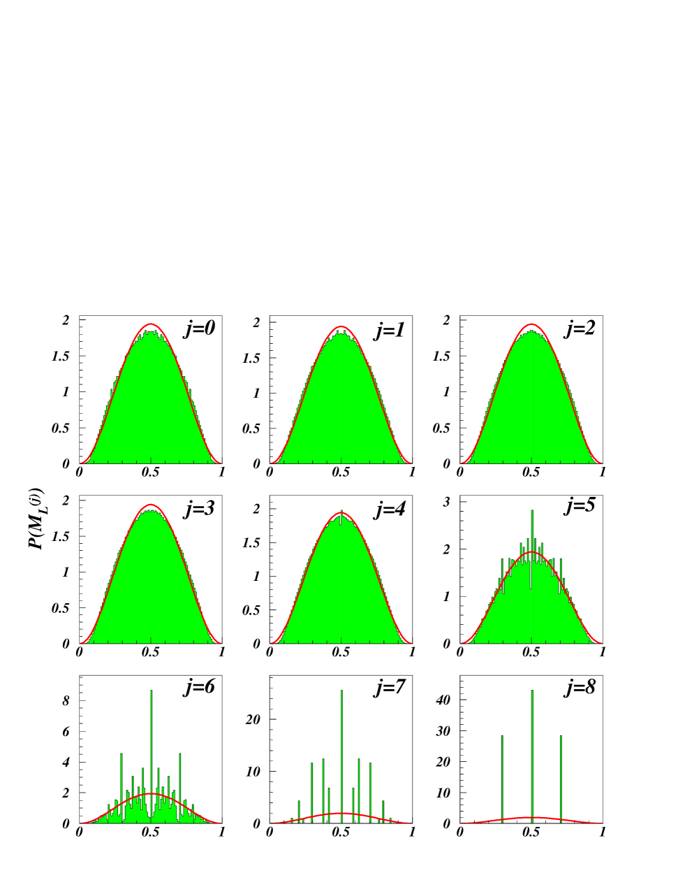
FIG. 1.: Convergence of the left multiplier distributions $p(M_{L}^{(j)})$ of the non-energy conserving $\alpha$-model (3) to a quasi-continuous limiting form. Parameters are $J=9$, $\alpha=0.3$ and $\beta=0.65$. For comparison the experimentally deduced Beta-function parametrisation of the left (right) unconditioned multiplier distribution with $\beta=3.2$ [8] is shown as a solid line.

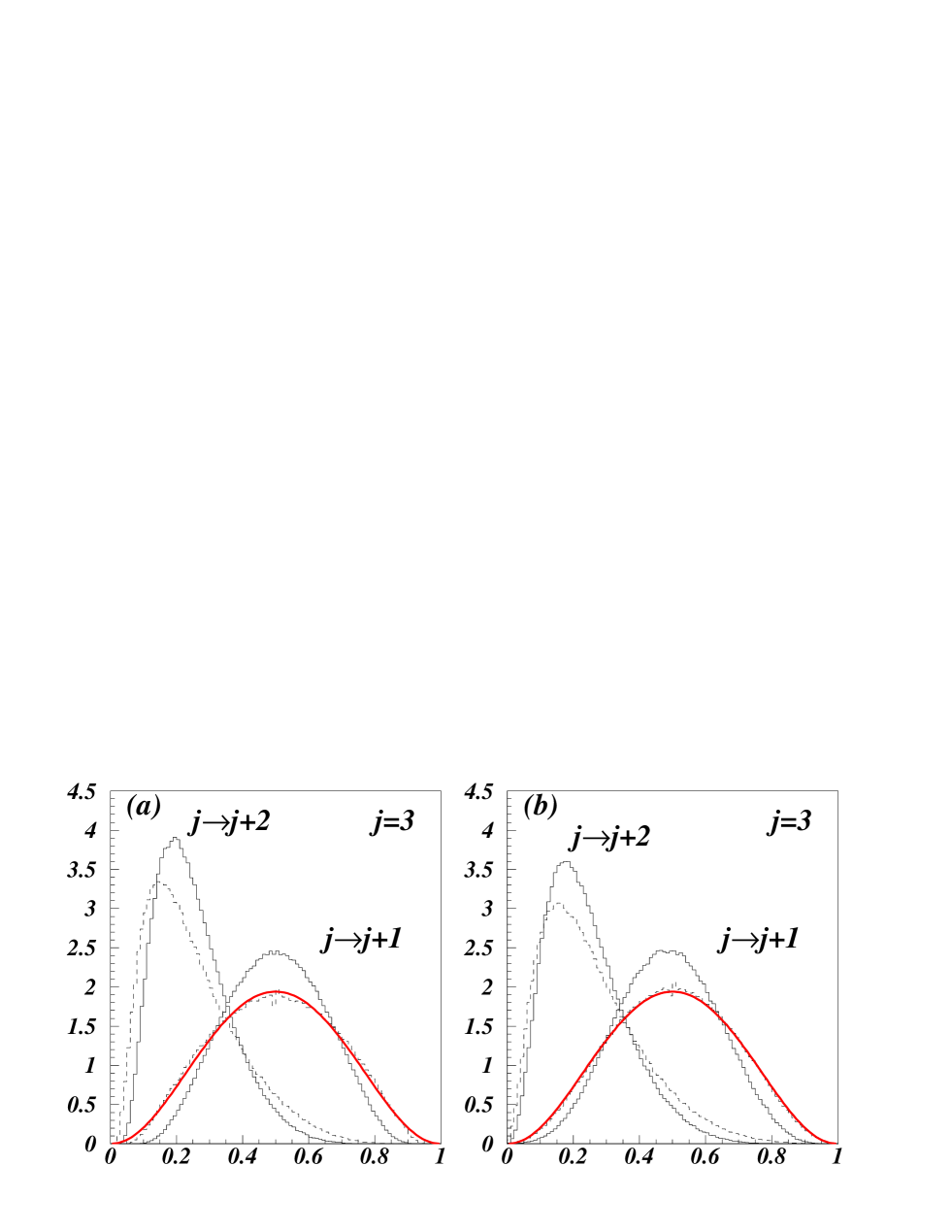
FIG. 2.: (a) Left (dashed) and centred (solid) multiplier distributions for the $\alpha$-model (3). For the one step multipliers $(j\rightarrow j+1)$ the length ratio between offspring and parent intervals is $\lambda=\frac{1}{2}$ while for the two-step multipliers $(j\rightarrow j+2)$ we have $\lambda=\frac{1}{4}$. Parameters are $J=9$, $\alpha=0.3$ and $\beta=0.65$.(b) Same as (a), but with random translations applied before calculating the multipliers. For comparison the experimentally deduced Beta-function parametrisation of the left (right) multiplier distribution $(j\rightarrow j+1)$ with $\beta=3.2$ [8] is shown as a thick solid line.

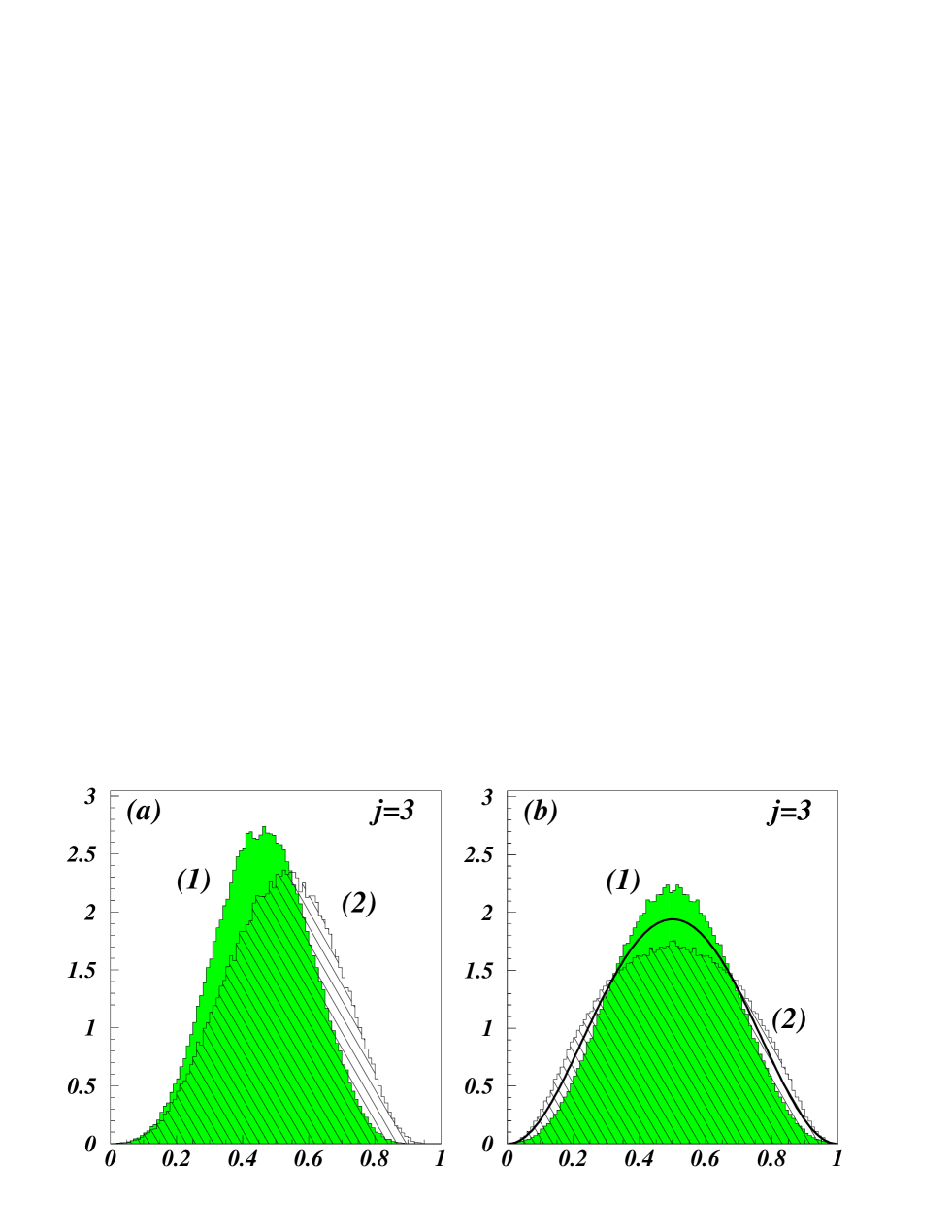
FIG. 3.: Conditioned multiplier distributions for the $\alpha$-model, satisfying strictly conditions (a) and (b) in the text. Parameters are $J=9$, $\alpha=0.3$, $\beta=0.65$ and random translations were applied before calculating the multipliers. (a) Central distributions conditioned on central parent multipliers: (1) $p(M^{(j)}_{C}|0\leq M^{(j-1)}_{C}\leq 1/2)$ and (2) $p(M^{(j)}_{C}|1/2<M^{(j-1)}_{C}\leq 1)$. (b) Left distributions conditioned on left parent multipliers: (1) $p(M^{(j)}_{L}|0.2\leq M^{(j-1)}_{L}\leq 0.4)$ and (2) $p(M^{(j)}_{L}|0.6\leq M^{(j-1)}_{L}\leq 0.8)$ compared to the Beta-function parametrisation of unconditioned distributions in Fig. 1 and Fig. 2 (full line).

- [1] U. Frisch, Turbulence (Cambridge University Press, Cambridge, 1995).
- [2] D. Schertzer and S. Lovejoy, in Turbulent Shear Flows 4, University of Karlsruhe (1983), edited by L.J.S. Bradbury and al (Springer, Berlin,1984).
- [3] C. Meneveau and K.R. Sreenivasan, Phys. Rev. Lett. 59, 1424 (1987).
- [4] E. A. Novikov, Appl. Math. Mech. 35, 231 (1971).
- [5] M. Greiner, H. C. Eggers and P. Lipa, preprint chao-dyn/9804024; M. Greiner, J. Schmiegel, F. Eickemeyer, P. Lipa and H. C. Eggers, preprint chao-dyn/9804028, Phys.Rev. E, in press.
- [6] C. Meneveau and K.R. Sreenivasan, J. Fluid Mech. 224, 429 (1991).
- [7] A. B. Chhabra and K. R. Sreenivasan, Phys. Rev. Lett. 68, 2762 (1992)
- [8] K.R. Sreenivasan and G. Stolovitzky, J. Stat. Phys. 78, 311 (1995).
- [9] G. Pedrizzetti, E.A. Novikov and A.A. Praskovsky, Phys. Rev. E53, 475 (1996).
- [10] M. Nelkin and G. Stolovitzky, Phys. Rev. E55, 5100 (1996).
- [11] M. Greiner, J. Giesemann, and P. Lipa, Phys. Rev. E 56, 4263 (1997).
- [12] M. Greiner, J. Giesemann, P. Lipa and P. Carruthers, Z. Phys. C 69, 305 (1996).
- [13] E. A. Novikov, Phys. Rev. E51, R3303 (1994).
- [14] B. Jouault, P. Lipa and M. Greiner, in preparation.
- [15] M. Greiner, P. Lipa and P. Carruthers, Phys. Rev. E 51, 1948 (1995).