Average Patterns of Spatiotemporal Chaos: A Boundary Effect

Abstract

Chaotic pattern dynamics in many experimental systems show structured time averages. We suggest that simple universal boundary effects underly this phenomenon and exemplify them with the Kuramoto-Sivashinsky equation in a finite domain. As in the experiments, averaged patterns in the equation recover global symmetries locally broken in the chaotic field. Plateus in the average pattern wavenumber as a function of the system size are observed and studied and the different behaviors at the central and boundary regions are discussed. Finally, the structure strenght of average patterns is investigated as a function of system size.

Experimental studies of the chaotic pattern dynamics in Faraday waves [3, 4], in rotating thermal convection [5], and in electroconvection [6], reveal that spatio-temporal complex patterns can have surprisingly ordered time averages. The form of these average patterns (square, circular, hexagonal) is determined by the underlying symmetry [7, 8] imposed by the boundary conditions. Although the instantaneous patterns fluctuate chaotically, they are biased towards the average pattern because they have short-lived patches spatially in phase with this average. This phase rigidity seems to come from the boundaries, and quantization effects appear due to the finite size of the container. The amplitude of the time-averaged pattern depends on the system size and control parameters. It is strongest near the sidewalls, and decays with increasing distance from the sidewalls and with increasing fluctuations about the ordered averaged state. For very large containers the ordered average pattern exists only near the sidewalls.

Given the general features of average patterns suggested by experiments, it seems surprising that their possible existence and characterization have not been addressed within the standard model equations displaying spatiotemporal chaotic states [9]. One possible reason for this is that periodic boundary conditions are usually considered in theoretical studies. In such situation spatial translational invariance homogenizes out any time average (unless some unexpected ergodicity breaking takes place). Boundary conditions breaking translational symmetry, as in the experiments, are thus needed to obtain nontrivial average patterns. Motivated by this fact, we here consider the Kuramoto-Sivashinsky equation, one of the prototype equations showing spatiotemporal chaos, in bounded one and two dimensional domains. We show that ordered average patterns do appear, despite the strong fluctuations, and we discuss the universal aspects of wave number selection and amplitude variations. More directly, our analysis of average patterns may be relevant and suggestive for experiments on phase turbulence in convection cells [10], fluids flowing down an inclined wall [11], and flame front propagation [12, 13].

The Kuramoto-Sivashinsky equation [10, 14] is perhaps the simplest partial differential equation exhibiting spatio-temporal chaos. The equation in one dimension has the form:

$$h_{t}=-h_{xx}-h_{xxxx}+(h_{x})^{2}~{},$$ (1)

where $h=h(x,t)$ is a real function, $x\in[0,L]$, and the subscripts stand for derivatives. In two dimensions the spatial derivative is replaced by a gradient and the second derivative by a Laplacian. The only control parameter for the equation is the length of the domain $L$; prefactors to the terms in Eq. (1) can be scaled out. An equivalent equation for $u=h_{x}$ can be obtained by taking the derivative of Eq. (1) with respect to $x$,

$$u_{t}=-u_{xx}-u_{xxxx}+2uu_{x}~{}.$$ (2)

Eq. (1) possesses translational symmetries ($h\to h+h_{0}$, $x\to x+x_{0}$) a reflexion symmetry ($h\to h$, $x\to-x$), and an infinitesimal Galilean symmetry ($x\to x+2vt$, $h\to h+vx$). Eq. (2) is also invariant under translations ($u\to u$, $x\to x+x_{0}$) and under a Galilean symmetry ($x\to x+2vt$, $u\to u+v$). A different reflexion symmetry is valid in this case ($u\to-u$, $x\to-x$).

The stability of the laminar solution $h=0$ ($u=0$) is analyzed by linearizing Eq. (1) [Eq. (2)]. For commonly used boundary conditions the growth rate $\mu$ for the Fourier mode of wavenumber $k$ is $\mu=k^{2}-k^{4}$. In two dimensions $k^{2}$ is replaced by $|{\bf k}|^{2}$. The laminar solution is unstable for all modes within $0<k<1$. The fastest growing mode has a wavenumber $k_{0}=1/\sqrt{2}$ corresponding to a wavelength $\lambda_{0}=2\sqrt{2}\pi\approx 8.9$. The wavelength $\lambda_{0}$ serves as a basic length scale, and the system size $L$ is naturally measured in units of this scale, $L/\lambda_{0}$, which is called the aspect ratio. Beyond the linear range, the nonlinear term becomes important and produces growth (linear in time) of the mean value of $h$, while the mean value of $u$ saturates. For $L$ large enough to permit a sufficient number of unstable Fourier modes, the solution exhibits spatio-temporal chaotic behavior that can be associated with a disordered evolution of a cellular pattern.

Many studies have been devoted to the bulk behavior of the Kuramoto-Sivashinsky system [9]. In relation to average patterns however the boundaries are of paramount importance, as discussed above. Here, we consider two types of boundary conditions. One of them is the rigid boundary conditions, where

$$u(0,t)=u(L,t)=u_{x}(0,t)=u_{x}(L,t)=0~{},$$ (3)

or equivalently,

$$h_{x}(0,t)=h_{x}(L,t)=h_{xx}(0,t)=h_{xx}(L,t)=0~{}.$$ (4)

Our other choice of boundary conditions is

$$u(0,t)=u(L,t)=u_{xx}(0,t)=u_{xx}(L,t)=0~{},$$ (5)

or equivalently,

$$h_{x}(0,t)=h_{x}(L,t)=h_{xxx}(0,t)=h_{xxx}(L,t)=0~{},$$ (6)

which we call stress-free boundary conditions, with reference to similar conditions in hydrodynamics.

We integrate the Kuramoto-Sivashinsky equation using explicit finite-differences of first order in time, second order in space for the linear terms, and fourth order in space for the nonlinear term. The time step is chosen sufficiently small to avoid any spurious behavior. The number of grid points used is $128$ in one dimensional simulations and $64\times 64$ in two dimensions. In all cases, the simulations were started from random initial conditions.

FIG. 1.: Results from simulations of the one-dimensional Kuramoto-Sivashinsky equation with stress-free boundary conditions. System size $L=70$. a) A characteristic front $\varphi$ at time $t=1000$. b) The time average of the front $\varphi$ (continuous line) and of $u$ (dashed).

We are interested in the average pattern of $u$ and the average pattern of the front $\varphi$ of $h$,

$$\varphi(x,t)=h(x,t)-\frac{1}{L}\int_{0}^{L}h(x,t)dx~{}.$$ (7)

To optimize the measurements of the average, the sampling was first started well beyond the initial transient behavior. For the system sizes considered, the typical transient time was limited to approximately $20$ time units, and we discarded the first $100$ time units. Then, averages where taken from configurations sampled every $5$ time units. A total of $10,000$ configurations per run were included, and further average over 10 runs with independent random initial conditions was performed. This is a large sample, but was necessary to compensate for the slow convergence of the averages produced by the long-range time correlations present in the KS equation.

FIG. 2.: The same as Fig. 1 but for rigid boundary conditions

.

In both one and two dimensions and with both rigid and stress-free boundary conditions we obtain non-trivial and ordered time-averaged patterns from the spatio-temporally chaotic evolution (Figs. 1-5), emphasizing that the formation of average patterns in spatio-temporal complex systems is general despite the presence of very large fluctuations. The presence of boundaries breaks the translational symmetry of the equations. The boundary conditions (3)-(6) respect however its reflection symmetries (for reflexions with respect to the center of the domain). As in the experiments, here we find that the average patterns display these remaining symmetries. In the two-dimensional case the average pattern recovers also the square symmetry of the integration domain (Fig. 3). Except for the one-dimensional case with stress-free boundary conditions (Fig. 1), an overall parabolic profile of the average front is obtained (see Figs. 2-4). For the derivative $u$ a mean slope is obtained [15]. This parabolic profile is a peculiarity of the Kuramoto-Sivashinsky equation. It can be removed by considering the second derivative of the front $\varphi$ instead of $\varphi$ itself; for this variable (and for the Laplacian in two dimensions) the discussion for all the cases is very similar to the one-dimensional stress-free situation, that we address in further detail in the remaining of the paper.

Fig. 5 shows the average patterns for $L=60$ and $L=100$. The number of oscillations increases with the size of the system, although only those close to the boundaries are large. Furthermore, the distance between consecutive maxima is close (but not equal, see below) to the characteristic length scale $\lambda_{0}\approx 8.9$. Similar observations were done in the experiments referred to at the beginning. In Fig. 6 the number of local maxima $N$ in the average front is shown for increasing values of the aspect ratio $L/\lambda_{0}$. $N$ is written in terms of the average distance $\lambda$ between two consecutive minima, $N=L/\lambda$. The line where $\lambda=\lambda_{0}$ is also indicated in Fig. 6. Plateaus are obtained at every integer $N$ between $6$ and $11$ for system sizes $L$ between $59$ and $112$. The average distance $\lambda$ is consistently larger than $\lambda_{0}$. Consistent deviations (positive or negative) are also known from the Faraday wave experiments [3].

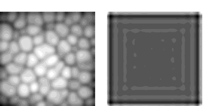
FIG. 3.: Results from simulations of the two-dimensional Kuramoto-Sivashinsky equation with stress-free boundary conditions. System size $L\times L=70\times 70$. Left: A characteristic instantaneous image of the front $\varphi$ ($t=1000$), different values of $\varphi$ are coded with different gray levels. Right: The average of $\nabla^{2}\varphi$, showing the square symmetry. The average of the Laplacian instead of the front itself is shown to eliminate the dominant parabolic shape of the average, thus improving the visibility of the sidewall oscillations.

If only the central region is considered, the plateaus fall off. More specifically, consider the ‘central region’, defined as the domain ranging from the second local minimum to the second last local minimum of $\varphi$ (see Fig. 5). The rest of the the pattern is thus considered the ‘boundary region’. We now determine the average distance $\lambda_{c}$ between consecutive minima in the central region for various system sizes $L$, and find the number of maxima $L/\lambda_{c}$ characteristic for the central region. The results are shown in Fig. 6. Intriguingly, the plateaus now fall off, an observation also done in experimental studies of the central region [3]. In order to explain this ‘fall off’ effect, we determine the average distance $\lambda_{b}$ between minima in the boundary regions. Over the entire range of system sizes considered, these distances changes very little, not more than 4%, so that to a first approximation we can consider $\lambda_{b}$ independent of $L$. For the central region we now have

$$\frac{L}{\lambda_{c}}=(N-4)\frac{L}{L-4\lambda_{b}}\simeq N+4\left(\frac{(N-4)\lambda_{b}}{L}-1\right)~{}.$$ (8)

The last approximation is valid for $\lambda_{b}/L$ small. For $\lambda_{b}$ constant, it is seen that $L/\lambda_{c}$ falls off as $\sim L^{-1}$ within a given plateau characterized by $N$. Thus an almost constant value of $\lambda_{b}$ serves as a generic explanation for the generally observed fall off of the plateaus. The overall picture is that when $L$ is increased the total number of oscillations tends to remain constant, as well as $\lambda_{b}$, so that $\lambda_{c}$ increases. This situation continues until the local wavelength in the central region is far enough from $\lambda_{0}$, moment at which a new oscillation is accommodated and a jump in $N$ occurs.

FIG. 4.: a) A central horizontal cut of the configuration shown in the left panel of Fig. 3. b) Solid: a central horizontal cut of the time average of the front $\varphi$ for the same parameter values; dashed: the same cut for the time average of $\varphi_{x}$.

From Fig. 5 it is clear that the amplitude $A(x)$ of the average pattern in general decays with increasing distance from the boundaries [16]. Experimental studies show the same behavior [3, 4, 5, 6]. To quantify this observation, we consider the spatial average $\left<A^{2}\right>=L^{-1}\int_{0}^{L}A^{2}dx$. The variation of $A_{rms}=\sqrt{\left<A^{2}\right>}$ with system size is shown in Fig. 7, showing a power-law dependence as $A_{rms}\sim L^{-1/2}$. We explain this fact by noting that Fig. 5 indicates that $A_{rms}$ receives its largest contribution from the boundaries, so that the integral in the definition of $\left<A^{2}\right>$ becomes a constant for system sizes larger than the boundary region. Thus the factor $L^{-1}$ in the definition of $\left<A^{2}\right>$ becomes the dominant $L$-dependence thus providing the observed behavior of $A_{rms}$.

In conclusion, we have established the formation of ordered time-averaged patterns in the Kuramoto-Sivashinsky equation, in one and two dimensions, and with rigid as well as stress-free boundary conditions. The average pattern recovers the symmetries which are respected by both the equation and the boundary conditions. The amplitude is strongest at the boundaries and decays with increasing distance to them. The law of decay has been found and explained. We have determined the selected wavelength $\lambda$, its variation with system size $L$, and interpreted the different behavior between the central and boundary regions. Most of these observations are also found in experimental systems for which the Kuramoto-Sivashinsky equation does not apply, thus indicating its generic, mainly geometrical, origin: What is relevant for these phenomena to occur is the occurrence of strong enough chaotic fluctuations in the presence of non-trivial boundaries.

We acknowledge the financial support of the Spanish Dirección General de Investigación Científica y Técnica, contract numbers PB94-1167 and PB94-1172.

FIG. 5.: Average patterns of the front $\varphi$ for the one-dimensional Kuramoto-Sivashinsky equation with stress-free boundary conditions. a) $L=60$. b) $L=100$. The arrows indicate the ‘central region’, as defined in the text.

FIG. 6.: +: The number of maxima $N=L/\lambda$ in the average front versus the aspect ratio $L/\lambda_{0}$, $\lambda$ being the average distance between consecutive minima in the entire region. $\diamond$: the number of maxima in the central region, given by $L/\lambda_{c}$. The solid line corresponds to $\lambda=\lambda_{0}$.

FIG. 7.: Variation of the root mean square amplitude $A_{rms}$ over the range of system sizes $59<L<107$. The solid curve is the function $C/\sqrt{L}$, with $C$ fitted to the data

REFERENCES

- [1] URL: http://www.imedea.uib.es/Nonlinear.
- [2] E-mail: victor@hp1.uib.es.
- [3] B.J. Gluckman, P. Marcq, J. Bridger and J.P. Gollub, Phys. Rev. Lett. 71, 2034 (1993); B.J. Gluckman, C.B. Arnold and J.P. Gollub, Phys. Rev. E 51, 1128 (1995).
- [4] E. Bosch, H. Lambermont and W. van de Water, Phys. Rev. E 49, 3580 (1994).
- [5] L. Ning, Y. Hu, R.E. Ecke and G. Ahlers, Phys. Rev. Lett. 71, 2216 (1993).
- [6] S. Rudroff and I. Rehberg, Phys. Rev. E 55, 2742 (1997).
- [7] P. Chossat and M. Golubitsky, Physica D 32, 423 (1988); M. Dellnitz, M. Golubitsky and I. Melbourne, in Bifurcation and symmetry, edited by E. Allgower, K. Bohmer and M. Golubitsky (Birkhauser, Basel, 1992), p. 99; M. Dellnitz, M. Golubitsky and I. Melbourne, Arch. Rat. Mech. Anal. 123, 75 (1993).
- [8] This symmetry-restoring phenomenon, induced here by chaotic fluctuations, has also been discussed in the context of stochastic fluctuations: P. Colet, M. San Miguel, M. Brambilla, L.A. Lugiato, Phys. Rev. A 43, 3862 (1991).
- [9] see e.g. M.C. Cross, P.C. Hohenberg, Rev. Mod. Phys. 65, 851 (1993).
- [10] Y. Kuramoto and T. Tsuzuki, Prog. Theor. Phys. 55, 356 (1976).
- [11] G.I. Sivashinsky and D.M. Michelson, Prog. Theor. Phys. 63, 2112 (1980).
- [12] G.I. Sivashinsky, Ann. Rev. Fluid Mech. 15, 170 (1983).
- [13] M. Gorman, private communication.
- [14] G.I. Sivashinsky, Acta Astronautica 4, 1177 (1977).
- [15] S. Zaleski and P. Lallemand, J. Phys. Lett. (Paris) 46, L793 (1985).
- [16] D.A. Egolf and H.S. Greenside, Phys. Lett. A 185, 395 (1994).