Universality in the random matrix spectra in the regime of weak non-Hermiticity

Abstract

Complex spectra of random matrices are studied in the regime of weak non-Hermiticity. The matrices we consider are of the form $\hat{H}_{1}+i\hat{H}_{2}$, where $\hat{H}_{1}$ and $\hat{H}_{2}$ are Hermitian and statistically independent. In the first part of the paper we consider the case of matrices $\hat{H}_{1,2}$ having i.i.d. entries. For such matrices the regime of weak non-Hermiticity is defined in the limit of large matrix dimension $N$ by the condition $\langle\mathop{\mathrm{Tr}}\hat{H}_{1}^{2}\rangle\propto N\langle\mbox{Tr}\hat{H}_{2}^{2}\rangle$. We show that in the regime of weak non-Hermiticity the distribution of complex eigenvalues of $\hat{H}_{1}+i\hat{H}_{2}$ is dictated by the global symmetries of $\hat{H}_{1,2}$, but otherwise is universal, i.e. independent of the particular distributions of their entries. Our heuristic proof is based on the supersymmetric technique and extends also to “invariant” ensembles of $\hat{H}_{1,2}$. In the second part of the paper we study Gaussian complex matrices in the regime of weak non-Hermiticity. Using the mathematically rigorous method of orthogonal polynomials we find the eigenvalue correlation functions. This allows us to obtain explicitly various eigenvalue statistics. These statistics describe a crossover from Hermitian matrices characterized by the Wigner-Dyson statistics of real eigenvalues to strongly non-Hermitian matrices whose complex eigenvalues were studied by Ginibre. Two-point statistical measures such as spectral form-factor, number variance and small distance behavior of the nearest neighbor distance distribution $p(s)$ are studied thoroughly. In particular, we found that the latter function may exhibit unusual behavior $p(s)\propto s^{5/2}$ for some parameter values.

I Introduction

Eigenvalues of large random matrices have been attracting much interest in theoretical physics since the 1950’s [1, 2, 3, 4, 5, 6, 7]. Until recently only the real eigenvalues were seen as physically relevant, hence most of the studies ignored matrices with complex eigenvalues. Powerful techniques to deal with real eigenvalues were developed and their statistical properties are well understood nowadays [2]. Microscopic justifications of the use of random matrices for describing the universal spectral properties of quantum chaotic systems have been provided by several groups recently, based both on traditional semiclassical periodic orbit expansions [8, 9] and on advanced field-theoretical methods [10, 11]. These facts make the theory of random Hermitian matrices a powerful and versatile tool of research in different branches of modern theoretical physics, see e.g.[4, 6, 7].

Recent studies of dissipative quantum maps [12, 13], asymmetric neural networks [14, 15], and open quantum systems [16, 17, 18, 19, 20] stimulated interest to complex eigenvalues of random matrices. Most obvious motivation comes from studies of resonances in open quantum systems, i.e. systems whose fragments can escape to or come from infinity. The resonances are determined as poles of the scattering matrix (S-matrix), as a function of energy of incoming waves, in the complex energy plane. The real part of the pole is the resonance energy and the imaginary part is the resonance half-width. Finite width implies finite life-time of the corresponding states. In the chaotic regime the resonances are dense and placed irregularly in the complex plane. Recently, the progress in numerical techniques and computational facilities made available resonance patterns of high accuracy for realistic open quantum chaotic systems like atoms and molecules [21].

Due to irregularity in the resonance widths and positions the S-matrix shows irregular fluctuations with energy and the main goal of the theory of the chaotic scattering is to provide an adequate statistical description of such a behavior. The so-called “Heidelberg approach” to this problem suggested in [22] makes use of random matrices. The starting point is a representation of the S-matrix in terms of an effective non-Hermitian Hamiltonian ${\cal H}_{eff}=\hat{H}-i\hat{\Gamma}$. The Hermitian $N\times N$ matrix $\hat{H}$ describes the closed counterpart of the open system and the skew-Hermitian $i\hat{\Gamma}=i\hat{W}\hat{W}^{T}$ arises due to coupling to open scattering channels $a=1,\ldots,M$, the matrix elements $W_{ja}$ being the amplitudes of direct transitions from ”internal” states $i=1,\ldots,N$ to one of open channels. The poles of the S-matrix coincide with the eigenvalues of ${\cal H}_{eff}$. In the chaotic regime one replaces $\hat{H}$ with an ensemble of random matrices of an appropriate symmetry. This step is usually “justified” by the common belief according to which the universal features of the chaotic quantum systems survive such a replacement [4, 5, 6, 7]. As a result, various features of chaotic quantum scattering can be efficiently studied by performing the ensemble averaging. The approach has proved to be very fruitful (for an account of recent developments see [20]). In particular, it allowed to obtain explicitly the distribution of the resonances in the complex plane for chaotic quantum systems with broken time-reversal invariance [19, 20] and, in its turn, this distribution was used to clarify some aspects of the relaxation processes in quantum chaotic systems[23].

A very recent outburst of interest to the non-Hermitian problems [24, 25, 26, 27, 28, 29, 30, 31, 32] deserves to be mentioned separately. During the last several years complex spectra of random matrices and operators emerged in a diversity of problems. Hatano and Nelson described depinning of flux lines from columnar defects in superconductors in terms of a localization-delocalization transition in non-Hermitian quantum mechanics [24]. Their work motivated a series of studies of the corresponding non-Hermitian Schrödinger operator [27, 28, 29, 30, 31] and, surprisingly, random matrices appeared to be relevant in this context [27, 28]. Complex eigenvalues were also discussed in the context of lattice QCD. The lattice Dirac operator entering the QCD partition function is non-Hermitian at nonzero chemical potential and proves to be difficult to deal with both numerically and analytically. Recent studies of chiral symmetry breaking used a non-Hermitian random matrix substitute for the Dirac operator [32]. There exist also interesting links between complex eigenvalues of random matrices and systems of interacting particles in one and two spatial dimensions [33]. And, finally, we have to mention that random matrices can be used for visualization of the pseudospectra of non-random convection-diffusion operators [34], and for description of two-level systems coupled to the noise reservoir[35].

Traditional mathematical treatment of random matrices with no symmetry conditions imposed goes back to the pioneering work by Ginibre[36] who determined all the eigenvalue correlation functions in an ensemble of complex matrices with Gaussian entries. The progress in the field was rather slow but steady [2, 37, 38, 39, 40, 41], see also [42, 43]. In addition to the traditional approach other aproaches have been developed and tested on new classes of non-Hermitian random matrices [15, 17, 19, 44, 45, 46, 47, 48]. However, our knowledge of the statistical properties of complex eigenvalues of random matrices is still far from being complete, in particular little is known about the universality classes of the obtained eigenvalue statistics.

When speaking about universality one has to specify the energy scale, for the degree of universality depends usually upon the chosen scale. There exist two characteristic scales in the random matrix spectra: the global one and the local one. The global scale is aimed at description of the distribution of the eigenvalues in bulk. The local one is aimed at decription of the statistical properties of small eigenvalue sets. For real spectra, the global scale is that on which a spectral interval of unit length contains on average a large, proportional to the matrix dimension, number of eigenvalues. If the spectrum is supported in a finite interval $[a,b]$ the global scale is simply given by the length of this interval. In contrary, the local scale is that determined by the mean distance $\Delta$ between two neighbouring eigenvalues. Loosely speaking, the local scale is $N$ times smaller than the global one sufficiently far from the spectrum edges, $N$ being the matrix dimension.

Universality in the real spectra is well established. The global scale universality is specific to random matrices with independent entries and does not extend to other classes of random matrices. The best known example of such universality is provided by the Wigner semicircle law [49]:

$$\langle\rho(X)\rangle=\frac{N}{2\pi J^{2}}\sqrt{4\,J^{2}-X^{2}}=N\nu(X)=\frac{1}{\Delta},$$ (1)

which holds for random matrices whose entries satisfy a Lindeberg type condition [50]. In this expression the parameter $J$ just sets the global scale in a sense as defined above. It is determined by the expectation value $J^{2}=\langle\frac{1}{N}\mathop{\mathrm{Tr}}\hat{H}^{2}\rangle$. It is generally accepted to scale entries in such a way that $J$ stays finite when $N\to\infty$, the local spacing between eigenvalues in the neighbourhood of the point $X$ being therefore $\Delta\propto 1/N$. Similar universality is also known for complex spectra [42, 43].

From the point of view of universality the semicircular eigenvalue density is not extremely robust. Most easily one violates it by considering an important class of so-called ”invariant ensembles” characterized by a probability density of the form ${\cal P}(\hat{H})\propto\exp{(-N\mathop{\mathrm{Tr}}V(\hat{H}))}$, with $V(\hat{H})$ being an even polynomial. The corresponding eigenvalue density turns out to be highly nonuniversal and determined by the particular form of the potential $V(H)$ [51, 52]. Only for $V(\hat{H})=\hat{H}^{2}$ it is given by the semicircular law, Eq.(1). Moreover, one can easily have a non-semicircular eigenvalue density even for real symmetric matrices $\hat{S};\quad S_{ij}=S_{ji}$ with i.i.d. entries, if one keeps the mean number of non-zero entries $p$ per column to be of the order of unity when performing the limit $N\to\infty$. This is a characteristic feature of the so-called sparse random matrices[53, 54, 55].

Much more profound universality emerges on the local scale in the real spectra. The statistical behavior of eigenvalues separated by distance $S=s\Delta$ measured in units of the mean eigenvalue spacing $\Delta$ is dictated by the global matrix symmetries (e.g. if they are complex Hermitian or real symmetric [2]), being the same for all random matrix ensembles within a fixed symmetry class. All ensemble specific information is encoded in $\Delta$. On different levels of rigor, this universality was established for “invariant” ensembles (i.e. matrices with invariant probabiltity distributions) [56, 57, 58] and for matrices with i.i.d. entries, including sparse matrices [54, 59]. Similar universality holds on a larger scale $S\gg\Delta$ [60, 61] and in the vicinity of the spectrum edges [62, 63].

It turns out, that it is the local scale universality that is mostly relevant for real physical systems[4]. Namely, statistics of highly excited bound states of closed quantum chaotic systems of quite different microscopic nature turn out to be independent of the microscopic details when sampled on the energy intervals large in comparison with the mean level separation, but smaller than the energy scale related by the Heisenberg uncertainty principle to the relaxation time necessary for a classically chaotic system to reach equilibrium in phase space [5]. Moreover, these statistics turn out to identical to those of large random matrices on the local scale, with different symmetry classes corresponding to presence or absence of time-reversal symmetry.

One of the aims of the present paper is to demonstrate that complex spectra of weakly non-Hermitian random matrices possess a universality property which is as robust as the above mentioned local scale universality in the real spectra of Hermitian matrices. Weakly non-Hermitian matrices appear naturally when one uses the Heidelberg approach to describe few-channel chaotic scattering [19]. When the number $M$ of open channels is small in comparison with the number $N$ of the relevant resonances, the majority of the S-matrix poles (resonances) are situated close to the real axis. This is well captured within the Heidelberg approach. With a proper normalization of $\hat{H}$ and $\hat{W}$, the imaginary part of typical eigenvalues of the effective Hamiltonian ${\cal H}_{eff}$ is of the order of the mean separation between neighboring eigenvalues along the real axis. This latter property is a characteristic feature of the regime of weak non-Hermiticity.

Motivated by this example we introduced in [45] another ensemble of weakly non-Hermitian random matrices. This ensemble consists of almost-Hermitian matrices which interpolate between the Gaussian ensemble of Hermitian matrices (GUE) and the Gaussian ensemble of complex matrices studied by Ginibre. It turned out that the eigenvalue distribution for almost-Hermitian random matrices is described by a formula [45] containing as two opposite limit cases both the Wigner semicircular distribution of real eigenvalues and the uniform distribution of complex eigenvalues obtained by Ginibre. Further studies of almost-Hermitian random matrices [41] showed that actually all their local scale eigenvalues statistics describe crossover between those of the GUE and Ginibre ensembles. Later on Efetov, in his studies of directed localization [27], discovered that weakly non-Hermitian matrices are relevant to the problem of motion of flux lines in superconductors with columnar defects. Efetov’s matrices are real almost-symmetric. They interpolate between Gaussian ensemble of real symmetric matrices (GOE) and the Gaussian ensemble of real asymmetric matrices. This development clearly shows that, apart from being a rich and largely unexplored mathematical object, weakly non-Hermitian random matrices enjoy direct physical applications and deserve a detailed study.

The present paper consists of two parts. In the first part we study a three parameter family of random matrix ensembles which contains the above mentioned ensembles of almost-Hermitian and almost-symmetric matrices. Our random matrices are of the form

$\displaystyle\hat{H}=(\hat{S}_{1}+iu\hat{A}_{1})+iv(\hat{S}_{2}+iw\hat{A}_{2}),$

where the four matrices on the right-hand side are mutually independent, with $\hat{S}_{1,2}$ being real symmetric and $\hat{A}_{1,2}$ being real skew-symmetric. By choosing matrix distributions and varying the parameter values one obtains different ensembles of non-Hermitian matrices. We use that normalization of matrix elements which ensures that

$\displaystyle\lim_{N\to\infty}\frac{1}{N}\langle\mathop{\mathrm{Tr}}S_{j}^{2}\rangle=\lim_{N\to\infty}\frac{1}{N}\langle\mathop{\mathrm{Tr}}A_{j}A_{j}^{T}\rangle=1,\;\;\;j=1,2$

$N$ being the matrix dimension. The parameters $v$ and $v$ are scaled with matrix dimension:

$\displaystyle v=\frac{\alpha}{2\sqrt{N}},\;\;\;\;u=\frac{\phi}{2\sqrt{N}},$

and $\alpha$, $\phi$, and $w$ are assumed to be of the order of unity in the limit $N\to\infty$. The above scaling of $v$ provides access to the regime of weak non-Hermiticity, while scaling $u$ we describe the crossover between the GOE and GUE types of behavior of eigenvalues of the Hermitian part of $\hat{H}$. A simple argument [45] based on the perturbation theory shows that for our random matrices the eigenvalue deviations from the real axis are of the order of $1/N$ when $N$ is large, i.e. it is of the same order as typical separation between real eigenvalues of the Hermitian $\hat{S}_{1}+iu\hat{A}_{1}$. Hence, in order to obtain a nontrivial eigenvalue distribution in the limit $N\to\infty$ one has to magnify the imaginary part scaling it with the matrix dimension.

Our study of the scaled eigenvalues of $\hat{H}$ is based on the supersymmetry technique. We express the density of the scaled eigenvalues in the form of a correlation function of a certain zero-dimensional non-linear $\sigma$-model. The obtained correlation function is given by a supersymmetric integral which involves only the density of the limit eigenvalue distribution of the Hermitian part of $\hat{H}$ and the parameters $\alpha$, $\phi$, $w$. In two particular cases this supersymmetric integral can be explicitly evaluated yielding the earlier obtained distributions of complex eigenvalues for almost-Hermitian [45, 41] and almost-symmetric matrices [27].

The supersymmetric $\sigma$-model was invented long ago by Efetov in the context of theory of disordered metals and the Anderson localization and since then have been successfully applied to diverse problems[64, 65]. Application of this technique to the calculation of the mean density of complex eigenvalues of non-Hermitian random matrices was done for the first time in our earlier works [19, 20, 45] and further advanced by Efetov [27] in the context of description of flux line motion in a disordered superconductor with columnar defects.

A detailed account of our calculations is given for sparse matrices [53, 54, 55] with i.i.d. entries, although our results are extended to “invariant” ensembles and conventional random matrices with i.i.d. entries. We assume that matrix entries of $\hat{S}_{k}$ and $\hat{A}_{k}$ are distributed on the real axis with the density

$${\cal P}(x)=\left(1-\frac{p}{N}\right)\delta(x)+\frac{p}{N}h(x),$$ (2)

where $h(x)$ is arbitrary symmetric density function, $h(x)=h(-x)$, having no delta function singularity at $x=0$ and satisfying the condition $\int x^{2}h(x)dx<\infty$. We also assume that the mean number of nonzero entries $p$ exceeds some threshold value: $p>p_{l}$, see [59].

We want to stress that Eq. (2) describes the most general class ofrandom matrices whose entries are i.i.d. variables with finite second moment[54]. In particular, in the first part of our paper we do not assume the matrix entries to be Gaussian.

We believe that here the power of the supersymmetry method is the most evident and we are not aware of any other analytical technique allowing to treat this general case non-perturbatively.

Although giving an important insight into the problem, the supersymmetry non-linear $\sigma-$model technique suffers from at least two deficiencies. The most essential one is that the present state of art in the application of the supersymmetry technique gives little hope of access to quantities describing correlations between different eigenvalues in the complex plane due to insurmountable technical difficulties. At the same time, conventional theory of random Hermitian matrices suggests that these universal correlations are the most interesting features. The second drawback is conceptual: the supersymmetry technique itself is not a rigorous mathematical tool at the moment and should be considered as a heuristic one from the point of view of a mathematician.

In the second part of the present paper we develop the rigorous mathematical theory of weakly non-Hermitian random matrices of a particular type: almost-Hermitian Gaussian. Our consideration is based on the method of orthogonal polynomials. Such a method is free from the above mentioned problem and allows us to study correlation properties of complex spectra to the same degree as is typical for earlier studied classes of random matrices. The results were reported earlier in a form of Letter-style communication[41]. Unfortunately, the paper [41] contains a number of misleading misprints. For this reason we indicate those misprints in the present text by using footnotes.

II Regime of Weak non-Hermiticity: Universal Density of Complex Eigenvalues

To begin with, any $N\times N$ matrix $\hat{J}$ can be decomposed into a sum of its Hermitian and skew-Hermitian parts: $\hat{J}=\hat{H}_{1}+i\hat{H}_{2},$ where $\hat{H}_{1}=(\hat{J}+\hat{J}^{\dagger})/2$ and $\hat{H}_{2}=(\hat{J}-\hat{J}^{\dagger})/2i$. Following this, we consider an ensemble of random $N\times N$ complex matrices $\hat{J}=\hat{H}_{1}+iv\hat{H}_{2}$ where $\hat{H}_{p};\,\,p=1,2$ are both Hermitian: $\hat{H}^{\dagger}_{p}=\hat{H}_{p}$. The parameter $v$ is used to control the degree of non-Hermiticity.

In turn, complex Hermitian matrices $\hat{H}_{p}$ can always be represented as $\hat{H}_{1}=\hat{S}_{1}+iu\hat{A}_{1}$ and $\hat{H}_{2}=\hat{S}_{2}+iw\hat{A}_{2}$, where $\hat{S}_{p}=\hat{S}_{p}^{T}$ is a real symmetric matrix, and $\hat{A}_{p}=-\hat{A}_{p}^{T}$ is a real antisymmetric one. From this point of view the parameters $u,w$ control the degree of being non-symmetric.

Throughout the paper we consider the matrices $\hat{S}_{1},\hat{S}_{2},\hat{A}_{1},\hat{A}_{2}$ to be mutually statistically independent, with i.i.d. entries normalized in such a way that:

$$\lim_{N\to\infty}\frac{1}{N}{\mbox{T}r}\hat{S}_{p}^{2}=\lim_{N\to\infty}\frac{1}{N}{\mbox{T}r}\hat{A}_{p}\hat{A}_{p}^{T}=1$$ (3)

As is well-known[4], this normalisation ensures, that for any value of the parameter $u\neq 0$ , such that $u=O(1)$ when $N\to\infty$, statistics of real eigenvalues of the Hermitian matrix of the form $\hat{H}=\hat{S}+iu\hat{A}$ is identical (up to a trivial rescaling) to that of $u=1$, the latter case known as the Gaussian Unitary Ensemble (GUE). On the other hand, for $u\equiv 0$ real eigenvalues of real symmetric matrix $S$ follow another pattern of the so-called Gaussian Orthogonal Ensemble (GOE).

The non-trivial crossover between GUE and GOE types of statistical behaviour happens on a scale $u\propto 1/N^{1/2}$[66]. This scaling can be easily understood by purely perturbative arguments[67]. Namely, for $u\propto 1/N^{1/2}$ the typical shift $\delta\lambda$ of eigenvalues of the symmetric matrix $S$ due to antisymmetric perturbation $iu\hat{A}$ is of the same order as the mean spacing $\Delta$ between unperturbed eigenvalues : $\delta\lambda\sim\Delta\sim 1/N$.

Similar perturbative arguments show[45], that the most interesting behaviour of complex eigenvalues of non-Hermitian matrices should be expected for the parameter $v$ being scaled in a similar way: $v\propto 1/N^{1/2}$. It is just the regime when the imaginary parts $\mathop{\mathrm{Im}}Z_{k}$ of a typical eigenvalue $Z_{k}$ due to non-Hermitian perturbation is of the same order as the mean spacing $\Delta$ between unperturbed real eigenvalues : $\mathop{\mathrm{Im}}Z_{k}\sim\Delta\sim 1/N$. Under these conditions a non-Hermitian matrix $J$ still ”remembers” the statistics of its Hermitian part $\hat{H}_{1}$. As will be clear afterwards, the parameter $w$ should be kept of the order of unity in order to influence the statistics of the complex eigenvalues.

It is just the regime of weak non-Hermiticity which we are interested in. Correspondingly, we scale the parameters as :

$$v=\frac{\alpha}{2\sqrt{N}};\quad u=\frac{\phi}{2\sqrt{N}}$$ (4)

and consider $\alpha,\phi,w$ fixed of the order O(1) when $N\to\infty$.

One can recover the spectral density

$$\rho(Z)=\sum_{k=1}^{N}\delta^{(2)}(Z-Z_{k})=\sum_{k=1}^{N}\delta(X-X_{k})\delta(Y-Y_{k})=\rho(X,Y)$$ (5)

of complex eigenvalues $Z_{k}=X_{k}+iY_{k},\quad k=1,2,...,N$ from the generating function (cf.[14, 20])

$${\cal Z}=\frac{{\mbox{D}et}\left[(Z-J)(Z-J)^{\dagger}+\kappa^{2}\right]}{{\mbox{D}et}\left[(Z_{b}-J)(Z_{b}-J)^{\dagger}+\kappa^{2}\right]}$$ (6)

as

$\displaystyle\rho(Z)=-\frac{1}{\pi}\lim_{\kappa\to 0}\frac{\partial}{\partial Z^{*}}\lim_{Z_{b}\to Z}\frac{\partial}{\partial Z_{b}}{\cal Z}.$

To facilitate the ensemble averaging we first represent the ratio of the two determinants in Eq.(6) as the Gaussian integral

$${\cal Z}=\int\prod_{i=1}^{N}[d\Phi_{i}]\exp\{{\cal L}_{1}(\Phi)+{\cal L}_{2}(\Phi)\}$$ (7)

over 8-component supervectors $\Phi_{i}$,

$\displaystyle\Phi_{i}=\left(\begin{array}[]{c}\Psi_{i}(+)\\ \Psi_{i}(-)\end{array}\right),\Psi_{i}(\pm)=\left(\begin{array}[]{c}\vec{R}_{i}(\pm)\\ \vec{\eta}_{i}(\pm)\end{array}\right),\vec{R}_{i}(\pm)=\left(\begin{array}[]{c}r_{i}(\pm)\\ r_{i}^{*}(\pm)\end{array}\right),\vec{\eta}_{i}(\pm)=\left(\begin{array}[]{c}\chi_{i}(\pm)\\ \chi_{i}^{*}(\pm)\end{array}\right)$

with components $r_{i}(+),r_{i}(-);\quad i=1,2,...,N$ being complex commuting variables and $\chi_{i}(+),\chi_{i}(-)$ forming the corresponding Grassmannian parts of the supervectors $\Psi_{i}(\pm)$. The terms in the exponent of Eq.(7) are of the following form:

$${\cal L}_{1}(\Phi) = -\frac{i}{2}\sum_{i}\Phi_{i}^{\dagger}\left\{S_{1,{ii}}\hat{\Lambda}\right\}\Phi_{i}-i\sum_{i<j}\Phi_{i}^{\dagger}\left\{S_{1,ij}\hat{\Lambda}\right\}\Phi_{j}$$ (8)

$${\cal L}_{2}(\Phi) = \frac{i}{2}\sum_{i}\Phi_{i}^{\dagger}\left\{X_{b}\hat{\Lambda}_{b}+X\hat{\Lambda}_{f}-i\kappa\hat{I}+iY_{b}\hat{\Sigma}_{\tau,b}+iY\hat{\Sigma}_{\tau,f}\right\}\Phi_{i}-$$ (10)

$$i\sum_{i<j}\Phi_{i}^{\dagger}\left\{ivS_{2,ij}\Sigma_{\tau}+iuA_{1,ij}\hat{\Lambda}_{\tau}+vwA_{1,ij}\hat{\Sigma}\right\}\Phi_{j}.$$

Here $\hat{I}_{2}=\mathop{\mathrm{diag}}(1,1)$, $\hat{I_{4}}=\mathop{\mathrm{diag}}(\hat{I}_{2},\hat{I}_{2})$, $\hat{\Lambda}=\mathop{\mathrm{diag}}(\hat{I}_{4},-\hat{I}_{4})$, $\hat{\Lambda}_{b}=\mathop{\mathrm{diag}}(\hat{I}_{2},\hat{0}_{2},-\hat{I}_{2},\hat{0}_{2})$, $\hat{\Lambda}_{f}=\hat{\Lambda}-\hat{\Lambda}_{b}$, $\hat{\Sigma}=\hat{\Sigma}_{b}+\hat{\Sigma}_{f}$, and

$\displaystyle\hat{\Sigma}_{b}=\left(\begin{array}[]{cc}\hat{0}_{4}&\left(\begin{array}[]{cc}\hat{I}_{2}&\hat{0}_{2}\\ \hat{0}_{2}&\hat{0}_{2}\end{array}\right)\\ \left(\begin{array}[]{cc}-\hat{I}_{2}&\hat{0}_{2}\\ \hat{0}_{2}&\hat{0}_{2}\end{array}\right)&{\hat{0}_{4}}\end{array}\right);\quad\quad\hat{\Sigma}_{f}=\left(\begin{array}[]{cc}\hat{0}_{4}&\left(\begin{array}[]{cc}\hat{0}_{2}&\hat{0}_{2}\\ \hat{0}_{2}&\hat{I}_{2}\end{array}\right)\\ \left(\begin{array}[]{cc}\hat{0}_{2}&\hat{0}_{2}\\ 0&-\hat{I}_{2}\end{array}\right)&\hat{0}_{4}\end{array}\right).$

and the matrices $\hat{\Sigma}_{\tau,b},\hat{\Sigma}_{\tau,f},\hat{\Sigma}_{\tau},\hat{\Lambda}_{\tau}$ are obtained from the corresponding matrices without subindex $\tau$ by replacing all $\hat{I}_{2}$ blocks with the matrices $\hat{\tau}=\mathop{\mathrm{diag}}(1,-1)$.

We also use $\vec{\eta}_{i}^{\dagger}(\pm)=\left(\chi_{i}^{*}(\pm);-\chi_{i}(\pm)\right)$. When writing ${\cal L}_{2}(\Phi)$ in Eq.(10) we have used the fact that diagonal matrix elements $S_{2,ii}$ for $i=1,..,N$ give total contribution of the order of $O(1/N)$ with respect to the total contribution of the off-diagonal ones and can be safely disregarded.

Now we should perform the ensemble averaging of the generating function. We find it to be convenient to average first over the distribution of matrix elements of the real symmetric matrix $\hat{S}_{1}$.

These elements are assumed to be distributed according to Eq.(2). Before presenting the derivation for our case, let us remind the general strategy. The procedure consists of three steps. First step is the averaging of the generation function over the disorder. It can be done trivially due to statistical independence of the matrix elements in view of the integrand being a product of exponents, each depending only on the particular matrix element $H_{ij}$. This averaging performed, the integrand ceases to be the simple Gaussian and thus the integration over the supervectors can not be performed any longer without further tricks.When matrix elements are Gaussian-distributed, this difficulty is circumvented in a standard way by exploiting the so-called Hubbard-Stratonovich transformation. That transformation amounts to making the integrand to be Gaussian with respect to components of the supervector by introducing new auxilliary integrations. After that the integral over supervectors can be performed exactly, and remaining auxilliary degrees of freedom are integrated out in the saddle-point approximation justified by large parameter $N$.

As is shown in the paper [54], there exists an analogue of the Hubbard-Stratonovich transformation allowing to perform the steps above also for the case of arbitrary non-Gaussian distribution. The main difference with the Gaussian case is that the auxilliary integration has to be chosen in a form of a functional integral .

Our presentation follow the procedure suggested in [54], and presented also in some detail in [55]

.

Exploiting the large parameter $N\gg 1$ one can write:

$$\left\langle\exp{{\cal L}_{1}(\Phi)}\right\rangle\mid_{N\gg 1}\approx\exp{\left[\frac{p}{2N}\sum_{i,j}h_{F}(\Phi_{i}^{\dagger}\hat{\Lambda}\Phi_{j})\right]};\quad h_{F}(z)=\int\limits_{-\infty}^{\infty}dsh(s)e^{-isz}-1$$ (11)

In order to proceed further we employ the functional Hubbard-Stratonovich transformation introduced in [54]:

$$\exp{\left[\frac{p}{2N}\sum_{i,j}h_{F}(\Phi_{i}^{\dagger}\hat{\Lambda}\Phi_{j})\right]}=$$ (13)

$$\int{\cal D}g\ \exp{\left[-\frac{pN}{2}\int d\Theta d\tilde{\Theta}g(\Theta)C(\Theta,\tilde{\Theta})g(\tilde{\Theta})+p\sum_{i=1}^{N}g(\Phi_{i})\right]}$$

where the kernel $C(\Theta,\tilde{\Theta})$ is determined by the relation:

$$\int d\tilde{\Theta}C(\Theta,\tilde{\Theta})h_{F}(\tilde{\Theta}\hat{\Lambda}\Phi)=\delta(\Theta,\Phi)$$ (14)

with the right-hand side of the eq.(14) being the $\delta-$function in the space of supervectors.

Substituting eq.(13) into averaged eq.(7) and changing the order of integrations over $[d\Phi]_{i}$ and ${\cal D}g$ one obtains the averaged generating function in the form:

$$\left\langle{\cal Z}\right\rangle=\int{\cal D}g\exp{\left[-N{\cal L}(g)+\delta{\cal L}(g)\right]}$$ (15)

where

$${\cal L}(g) = \frac{p}{2}\int[d\Phi][d\tilde{\Phi}]\ g(\Phi)C(\tilde{\Phi},\Phi)g(\Phi)-\ln{\int[d\Phi]\ e^{{\cal F}(\Phi)}}$$ (16)

$$\delta{\cal L}(g) = \ln\ \frac{\int\prod_{i=1}^{N}[d\Phi_{i}]\ \exp{\left[\sum_{i}{\cal F}(\Phi_{i})+R\{\Phi\}\right]}}{\int\prod_{i=1}^{N}[d\Phi_{i}]\ \exp{\left[\sum_{i}{\cal F}(\Phi_{i})\right]}}$$ (17)

with ${\cal F}(\Phi)=\frac{i}{2}X\Phi^{\dagger}\hat{\Lambda}\Phi+pg(\Phi)$,

$\displaystyle R\{\Phi\}=\frac{1}{2}\sum_{i=1}^{N}\Phi_{i}^{\dagger}\hat{f}\Phi_{i}-i\sum_{i<j}\Phi_{i}^{\dagger}\left\{ivS_{2,ij}\hat{\Sigma}_{\tau}+iuA_{1,ij}\hat{\Lambda}_{\tau}+vwA_{1,ij}\hat{\Sigma}\right\}\Phi_{j},$

and $\hat{f}=\kappa\hat{I}-i(X-X_{b})\hat{\Lambda}_{b}-Y_{b}\hat{\Sigma}_{\tau,b}-Y\hat{\Sigma}_{\tau,f}$.

We are interested in evaluating the functional integral over ${\cal D}g$ in the limit $N\to\infty$ and $\kappa\to 0;X\to X_{b}$. Moreover, we expect eigenvalues of weakly non-Hermitian matrices to have imaginary parts $Y$ to be of the order of $1/N$. Remembering also the chosen scaling (4), we conclude that the argument of the logarithm in Eq.(17) is close to unity and the term $\delta{\cal L}(\Phi)$ in Eq.(15) should be treated as a small perturbation to the first one. Then the functional integral of the type $\int{\cal D}g(...)\exp{-N{\cal L}(g)}$ can be evaluated by the saddle-point method. Variating the ”action” ${\cal L}(g)$ and using the relation eq.(14) one obtains the following saddle point equation $\delta{\cal L}(g)/\delta g=0$ for the function $g(\Phi)$:

$$g(\Phi)=\frac{\int[d\Theta]h_{F}(\Phi^{\dagger}\hat{L}\Theta)\exp{{\cal F}(\Theta)}}{\int[d\Theta]\exp{{\cal F}(\Theta)}}$$ (18)

A quite detailed investigation of the properties of this equation was performed in [54, 55]. Below we give a summary of the main features of the eq.(18) following from such an analysis.

First, the solution $g(\Phi)$ to this equation can be sought for in a form of a function $g_{s}(\Phi)=g_{0}(x,y)$ of two superinvariants: $x=\Phi^{\dagger}\Phi$ and $y=\Phi^{\dagger}\hat{\Lambda}\Phi$.

As the result, the denominator in eq.(18) is equal to $1$ due to the identity $\int[d\Phi]F(x,y)=F(0,0)$ which is a particular case of the so-called Parisi-Sourlas-Efetov-Wegner (PSEW) theorem, see e.g.[65] and references therein. However, the form of the function $g_{0}(x,y)$ is essentially different for the number of nonzero elements $p$ per matrix column exceeding the threshold value $p=p_{l}$ and for $p<p_{l}$ [54, 59]. Namely, for $p>p_{l}$ the function $g_{0}(x,y)$ is an analytic function of both arguments $x$ and $y$, whereas for $p<p_{l}$ such a function is dependent only on the second argument $y=\Phi^{\dagger}\hat{\Lambda}\Phi$. At the same time, the saddle-point equation eq.(18) is always invariant w.r.t. any transformation $g(\Phi)\to g(\tilde{T}\Phi)$ with supermatrices $\tilde{T}$ satisfying the condition $\tilde{T}^{\dagger}\hat{\Lambda}\tilde{T}=\hat{\Lambda}$.

Combining all these facts together one finds, that for $p>p_{l}$ a saddle-point solution $g_{s}(\Phi)$ gives rise to the whole continuous manifold of saddle-point solutions of the form: $g_{T}(\Phi)\equiv g_{s}(\tilde{T}\Phi)=g_{0}(\Phi^{\dagger}\tilde{T}\tilde{T}\Phi,\Phi^{\dagger}\hat{\Lambda}\Phi)$, so that all the manifold gives a nonvanishing contribution to the functional integral eq.(15). It is the existence of the saddle-point manifold that is actually responsible for the universal random-matrix correlations[54].

We see, that the saddle-point manifold is parametrized by the supermatrices $\tilde{T}$. It turns out, however, that one has to ”compactify” the manifold of $\tilde{T}$ matrices with respect to the ”fermion-fermion” block in order to ensure convergence of the integrals over the saddle-point manifolds[22]. The resulting ”compactified” matrices $\hat{T}$ form a graded Lie group $\mbox{UOSP}(2,2/4)$. Properties of such matrices can be found in [22] together with the integration measure $d\mu(T)$.

¿From now on we are going to consider only the case $p>p_{l}$. The program of calculation is as follows: (i) To find the expression for the term $\delta{\cal L}(g)$ on the saddle-point manifold $g=g_{T}(\Phi)$ in the limit $N\to\infty$ and (ii) to calculate the integral over the saddle-point manifold exactly.

Expanding the expression in Eq. (17) to the first non-vanishing order in $\hat{f},\hat{S}_{2},\hat{A}_{1},\hat{A}_{2}$, introducing the notation ${\cal F}_{T}(\Phi)=\frac{i}{2}X\Phi^{\dagger}\hat{\Lambda}\Phi+pg_{T}(\Phi)$ and using the relations

$$\begin{array}[]{c}\int[d\Phi]\exp{{\cal F}_{T}(\Phi)}=1;\quad\int\prod_{k=1}^{N}[d\Phi_{k}]\left(\Phi^{\dagger}_{i}\hat{B}\Phi_{j}\right)|_{i<j}\exp{\sum_{k=1}^{N}{\cal F}_{T}(\Phi_{k})}=0;\\ \\ \int\prod_{k=1}^{N}[d\Phi_{k}]\left(\Phi^{\dagger}_{i_{1}}\hat{B}\Phi_{j_{1}}\right)|_{i_{1}<j_{1}}\left(\Phi_{i_{2}}^{\dagger}\hat{C}\Phi_{j_{2}}\right)|_{i_{2}<j_{2}}\exp{\sum_{k=1}^{N}{\cal F}_{T}(\Phi_{k})}\\ =\delta_{i_{1}i_{2}}\delta_{j_{1}j_{2}}\int[d\Phi_{i_{1}}][d\Phi_{j_{1}}]\left(\Phi^{\dagger}_{i_{1}}\hat{B}\Phi_{j_{1}}\right)\left(\Phi_{i_{1}}^{\dagger}\hat{C}\Phi_{j_{1}}\right)_{i_{1}<j_{1}}\exp{\left[{\cal F}_{T}(\Phi_{i_{1}})+{\cal F}_{T}(\Phi_{j_{1}})\right]}\end{array}$$ (19)

which hold for arbitrary $8\times 8$ supermatrices $\hat{B},\hat{C}$, one finds that

$$\delta{\cal L}(g_{T})=\frac{1}{2}\langle\Phi^{\dagger}\hat{f}\Phi\rangle_{T}+\delta{\cal L}_{R}+\delta{\cal L}_{IR},$$ (20)

where

$$\delta{\cal L}_{R} = \frac{v^{2}}{2}\sum_{i<j}\left(\hat{S}_{2}\right)^{2}_{ij}\left\langle\left[\Phi_{1}^{\dagger}\hat{\Sigma}_{\tau}\Phi_{2}\right]\left[\Phi_{1}^{\dagger}\hat{\Sigma}_{\tau}\Phi_{2}\right]\right\rangle_{T}$$

$$+ \frac{u^{2}}{2}\sum_{i<j}\left(\hat{A}_{1}\right)^{2}_{ij}\left\langle\left[\Phi_{1}^{\dagger}\Lambda_{\tau}\Phi_{2}\right]\left[\Phi_{1}^{\dagger}\hat{\Lambda}_{\tau}\Phi_{2}\right]\right\rangle_{T}-\frac{v^{2}w^{2}}{2}\sum_{i<j}\left(\hat{A}_{2}\right)^{2}_{ij}\left\langle\left[\Phi_{1}^{\dagger}\hat{\Sigma}\Phi_{2}\right]\left[\Phi_{1}^{\dagger}\hat{\Sigma}\Phi_{2}\right]\right\rangle_{T},$$

$$\delta{\cal L}_{IR} = uv\sum_{i<j}\left(\hat{S}_{2}\right)_{ij}\left(\hat{A}_{1}\right)_{ij}\left\langle\left[\Phi_{1}^{\dagger}\hat{\Sigma}_{\tau}\Phi_{2}\right]\left[\Phi_{1}^{\dagger}\hat{\Lambda}_{\tau}\Phi_{2}\right]\right\rangle_{T}-iv^{2}w\sum_{i<j}\left(\hat{S}_{2}\right)_{ij}\left(\hat{A}_{2}\right)_{ij}\left\langle\left[\Phi_{1}^{\dagger}\hat{\Sigma}_{\tau}\Phi_{2}\right]\left[\Phi_{1}^{\dagger}\hat{\Sigma}\Phi_{2}\right]\right\rangle_{T}$$

$$- iuvw\sum_{i<j}\left(\hat{A}_{1}\right)_{ij}\left(\hat{A}_{2}\right)_{ij}\left\langle\left[\Phi_{1}^{\dagger}\hat{\Lambda}_{\tau}\Phi_{2}\right]\left[\Phi_{1}^{\dagger}\hat{\Sigma}\Phi_{2}\right]\right\rangle_{T}$$

and we used the notations:

$$\left\langle\left[\Phi^{\dagger}\hat{B}\Phi\right]\right\rangle_{T} = \int[d\Phi]\left(\Phi^{\dagger}\hat{B}\Phi\right)e^{{\cal F}_{T}(\Phi)}$$

$$\left\langle\left[\Phi_{1}^{\dagger}\hat{B}\Phi_{2}\right]\left[\Phi_{1}^{\dagger}\hat{C}\Phi_{2}\right]\right\rangle_{T} = \int[d\Phi_{1}][d\Phi_{2}]\left(\Phi^{\dagger}_{1}\hat{B}\Phi_{2}\right)\left(\Phi_{1}^{\dagger}\hat{C}\Phi_{2}\right)\exp{\left[{\cal F}_{T}(\Phi_{1})+{\cal F}_{T}(\Phi_{2})\right]}.$$

It is clear that with the chosen normalization [see Eqs. (3) – (4)] we have

$$v^{2}\sum_{i<j}\left(\hat{S}_{2}\right)^{2}_{ij}\to\frac{\alpha^{2}}{8};\quad u^{2}\sum_{i<j}\left(\hat{A}_{1}\right)^{2}_{ij}\to\frac{\phi^{2}}{8};\quad w^{2}v^{2}\sum_{i<j}\left(\hat{A}_{2}\right)^{2}_{ij}\to\frac{w^{2}\phi^{2}}{8}$$ (21)

when $N\to\infty$. On the other hand, it is easy to see that:

$$uv\sum_{i<j}\left(\hat{S}_{2}\right)_{ij}\left(\hat{A}_{1}\right)_{ij}\sim wv^{2}\sum_{i<j}\left(\hat{S}_{2}\right)_{ij}\left(\hat{A}_{2}\right)_{ij}\sim wuv\sum_{i<j}\left(\hat{A}_{1}\right)_{ij}\left(\hat{A}_{2}\right)_{ij}=O(\frac{1}{N})$$ (22)

because of the statistical independence of $\hat{S}_{2},\hat{A}_{1},\hat{A}_{2}$ and the chosen normalization of matrix elements. Therefore, the part $\delta{\cal L}_{IR}$ can be safely neglected in the limit of large $N$.

To proceed further it is convenient to introduce the $8\times 8$ supermatrix $W$ with elements

$$W_{\alpha\beta}\equiv\int[d\Phi]\ \Phi_{\alpha}\Phi_{\beta}^{\dagger}e^{{\cal F}_{T}(\Phi)}$$ (23)

Exploiting the saddle-point equation for the function $g_{T}(\Phi)=g_{0}\left(\Phi^{\dagger}\hat{T}^{\dagger}\hat{T}\Phi,\Phi^{\dagger}\Lambda\Phi\right)$ one can show (details can be found in [55], Eqs.(67-70)) that the supermatrix $\hat{W}$ whose elements are $W_{\alpha\beta}$ can be written as:

$$\hat{W}=\frac{2}{B}\left[g_{0y}\hat{\Lambda}+ig_{0x}\hat{\Lambda}\hat{Q}\right]$$ (24)

where $B$ is the second moment of the distribution $h(s)$: $B=\int h(s)s^{2}ds$ and $g_{0x}=\partial g_{0}/\partial x|_{x=y=0};\quad g_{0y}=\partial g_{0}/\partial y|_{x=y=0}$. In the expression above we introduced a new supermatrix: $\hat{Q}=-i\hat{T}^{-1}\hat{\Lambda}\hat{T}$.

Using the definition of the matrix $W$, one can rewrite the part $\delta{\cal L}_{R}$ as follows (cf.[55], eqs. (71)-(73)):

$$\delta{\cal L}_{R}=-\frac{1}{16}\left[\alpha^{2}\mathop{\mathrm{Str}}\hat{W}\hat{\Sigma}_{\tau}\hat{W}\hat{\Sigma}_{\tau}-\phi^{2}\mathop{\mathrm{Str}}\hat{W}\hat{\Lambda}_{\tau}\hat{W}\hat{\Lambda}_{\tau}+w^{2}\phi^{2}\mathop{\mathrm{Str}}\hat{W}\hat{\Sigma}\hat{W}\hat{\Sigma}\right]$$ (25)

Now one can use Eq.(23) together with the properties: $\mathop{\mathrm{Str}}\hat{Q}=\mathop{\mathrm{Str}}\hat{\Lambda}=\mathop{\mathrm{Str}}\hat{I}=0;\quad Q^{2}=-\hat{I}$ to show that:

$\displaystyle\delta{\cal L}_{R}=\frac{g_{0x}^{2}}{4B^{2}}\left[\alpha^{2}\mathop{\mathrm{Str}}\hat{Q}\hat{\sigma}_{\tau}\hat{Q}\hat{\sigma}_{\tau}-\phi^{2}\mathop{\mathrm{Str}}\hat{Q}\hat{\tau}_{2}\hat{Q}\hat{\tau}_{2}+w^{2}\phi^{2}\mathop{\mathrm{Str}}\hat{Q}\hat{\sigma}\hat{Q}\hat{\sigma}\right]$

where the $8\times 8$ supermatrices entering these expressions are as follows:

$\displaystyle\hat{\tau}_{2}=\mathop{\mathrm{diag}}\{\hat{\tau}_{3},\hat{\tau}_{3}\};\quad\hat{\sigma}_{\tau}=\left(\begin{array}[]{cc}0&\hat{\tau}_{3}\\ \hat{\tau}_{3}&0\end{array}\right);\quad\hat{\sigma}=\left(\begin{array}[]{cc}0&\hat{I}_{4}\\ \hat{I}_{4}&0\end{array}\right)$

and $\hat{\tau}_{3}$ is $4\times 4$ diagonal, $\hat{\tau}_{3}=\mathop{\mathrm{diag}}\{\hat{\tau},\hat{\tau}\}$.

In the same way one finds:

$$\left\langle\Phi^{\dagger}\hat{f}\Phi\right\rangle_{T} = -\frac{4ig_{0y}}{B}(X-X_{b})+$$

$$\frac{2ig_{0x}}{B}\left[\kappa\mathop{\mathrm{Str}}\hat{Q}\hat{\Lambda}-i(X-X_{b})\mathop{\mathrm{Str}}\hat{K}_{B}\hat{Q}-Y_{B}\mathop{\mathrm{Str}}\hat{\sigma}_{\tau}^{(B)}\hat{Q}-Y\mathop{\mathrm{Str}}\hat{\sigma}_{\tau}^{(F)}\hat{Q}\right],$$

where

$\displaystyle\hat{K}_{B}=\mathop{\mathrm{diag}}\{\hat{I}_{2},\hat{0}_{2},\hat{I}_{2},\hat{0}_{2}\};\quad\hat{\sigma}_{\tau}^{(B,F)}=\left(\begin{array}[]{cc}\hat{0}_{4}&\hat{\tau}_{3}^{(B,F)}\\ \hat{\tau}_{3}^{(B,F)}&\hat{0}_{4}\end{array}\right)$

and $\hat{\tau}_{3}^{B,F}$ are $4\times 4$ diagonal supermatrices: $\hat{\tau}_{3}^{(B)}=\mathop{\mathrm{diag}}\{\hat{\tau},\hat{0}_{2}\}$ and $\hat{\tau}_{3}^{(F)}=\mathop{\mathrm{diag}}\{\hat{0}_{2},\hat{\tau}\}$.

At last, we use the relation between $g_{0}(x,y)$ and the mean eigenvalue density for a sparse symmetric matrix $\hat{S}_{1}$ at the point $X$ on the real axis derived in [54]:

$$\nu(X)\equiv\frac{1}{N}\langle\rho(X)\rangle=-\frac{2}{\pi B}g_{0x}$$ (26)

Substituting expressions for $\delta{\cal L}_{R}$ and $\left\langle\Phi^{\dagger}\hat{f}\Phi\right\rangle_{T}$ to the generating function ${\cal Z}$ represented as an integral over the saddle-point manifold parametrized by the supermatrices $\hat{T}$ (or, equivalently, by the supermatrices $\hat{Q}=-i\hat{T}^{-1}\hat{\Lambda}\hat{T}$) and performing the proper limits we finally obtain:

$$\langle\rho(X,Y)\rangle=\frac{\pi[N\nu(X)]^{2}}{16}\int d\mu(\hat{Q})\mathop{\mathrm{Str}}\left(\hat{\sigma}_{\tau}^{(F)}\hat{Q}\right)\mathop{\mathrm{Str}}\left(\hat{\sigma}_{\tau}\hat{Q}\right)\exp{-S(\hat{Q})}$$ (27)

$\displaystyle S(\hat{Q})=-\frac{i}{2}y\mathop{\mathrm{Str}}\left(\hat{\sigma}_{\tau}\hat{Q}\right)-\frac{a^{2}}{16}\mathop{\mathrm{Str}}\left(\hat{\sigma}_{\tau}\hat{Q}\right)^{2}+\frac{b^{2}}{16}\mathop{\mathrm{Str}}\left(\hat{\tau}_{2}\hat{Q}\right)^{2}-\frac{c^{2}}{16}\mathop{\mathrm{Str}}\left(\hat{\sigma}\hat{Q}\right)^{2}$

where we introduced the scaled imaginary parts $y=\pi\nu(X)NY$ and used the notations: $a^{2}=\left(\pi\nu(X)\alpha\right)^{2},\quad b^{2}=\left(\pi\nu(X)\phi\right)^{2},\quad c^{2}=\left(\pi\nu(X)\alpha w\right)^{2}$

The expression (27) is just the universal $\sigma-$ model representation of the mean density of complex eigenvalues in the regime of weak non-Hermiticity we were looking for. The universality is clearly manifest: all the particular details about the ensembles entered only in the form of mean density of real eigenvalues $\nu(X)$. The density of complex eigenvalues turns out to be dependent on three parameters: $a,b$ and $c$, controlling the degree of non-Hermiticity ($a$), and symmetry properties of the Hermitian part ($b$) and non-Hermitian part ($c$).

The following comment is appropriate here. The derivation above was done for ensembles with i.i.d. entries. However, one can satisfy oneself that the same expression would result if one start instead from any ”rotationally invariant” ensemble of real symmetric matrices $\hat{S}_{1}$. To do so one can employ the procedure invented by Hackenbroich and Weidenmüller [58] allowing one to map the correlation functions of the invariant ensembles (plus perturbations) to that of Efetov’s $\sigma-$model.

Still, in order to get an explicit expression for the density of complex eigenvalues one has to evaluate the integral over the set of supermatrices $\hat{Q}$. In general, it is an elaborate task due to complexity of that manifold.

At the present moment such an evaluation was successfully performed for two important cases: those of almost-Hermitian matrices and real almost-symmetric matrices. The first case ( which is technically the simplest one) corresponds to $\phi\to\infty$, that is $b\to\infty$. Under this condition only that part of the matrix $\hat{Q}$ which commutes with $\hat{\tau}_{2}$ provides a nonvanishing contribution. As the result, $\mathop{\mathrm{Str}}\left(\hat{\sigma}\hat{Q}\right)^{2}=\mathop{\mathrm{Str}}\left(\hat{\sigma}_{\tau}\hat{Q}\right)^{2}$ so that second and fourth term in Eq.(27) can be combined together. Evaluating the resulting integral, and introducing the notation $\tilde{a}^{2}=a^{2}+c^{2}$ one finds [45]:

$$\rho_{X}(y)=\sqrt{\frac{2}{\pi}}\frac{1}{\tilde{a}}\exp\left(-\frac{2y^{2}}{\tilde{a}^{2}}\right)\int\limits_{0}^{1}dt\cosh(2ty)\exp{(-\tilde{a}^{2}t^{2}/2)},$$ (28)

where $\rho_{X}(y)$ is the density of the scaled imaginary parts $y$ for those eigenvalues, whose real parts are situated around the point $X$ of the spectrum. It is related to the two-dimensional density as $\rho_{X}(y)=\rho(X,Y)/\pi(N\nu(X))^{2}$.

It is easy to see, that when $\tilde{a}$ is large one can effectively put the upper boundary of integration in Eq.(28) to be infinity due to the Gaussian cut-off of the integrand. This immediately results in the uniform density $\rho_{X}(y)=(\tilde{a}^{2})^{-1}$ inside the interval $|y|<\tilde{a}^{2}/2$ and zero otherwise. Translating this result to the two-dimensional density of the original variables $X,Y$, we get:

$$\rho(X,Y)=\left\{\begin{array}[]{ll}\displaystyle{\frac{N}{4\pi v^{2}(1+w^{2})}}&\mbox{if}\,\,\displaystyle{|Y|\leq 2\pi\nu(X)v^{2}(1+w^{2})}\\ 0&\mbox{otherwise}\end{array}\right.$$ (29)

This result is a natural generalisation of the so-called ”elliptic law” known for strongly non-Hermitian random matrices[36, 14]. Indeed, the curve encircling the domain of the uniform eigenvalue density is an ellipse: $\frac{Y^{2}}{2v^{2}(1+w^{2})}+\frac{X^{2}}{4}=1$ as long as the mean eigenvalue density of the Hermitian counterpart is given by the semicircular law, Eq.(1) (with the parameter $J=1$). The semicircular density is known to be shared by ensembles with i.i.d. entries, provided the mean number $p$ of non-zero elements per row grows with the matrix size as $p\propto N^{\alpha};\,\,\alpha>0$, see [54]. In the general case of sparse or ”rotationally invariant” ensembles the function $\nu(X)$ might be quite different from the semicircular law. Under these conditions Eq.(29) still provides us with the corresponding density of complex eigenvalues.

The second nontrivial case for which the result is known explicitly is due to Efetov[27]. It is the limit of slightly asymmetric real matrices corresponding in the present notations to: $\phi\to 0;w\to\infty$ in such a way that the product $\phi w=\tilde{c}$ is kept fixed. The density of complex eigenvalues turns out to be given by:

$$\rho_{X}(y) = \delta(y)\int\limits_{0}^{1}dt\exp{(-\tilde{c}^{2}t^{2}/2)}$$ (30)

$$+2\sqrt{\frac{2}{\pi}} \frac{|y|}{\tilde{c}}\int\limits_{1}^{\infty}du\exp\left(-\frac{2y^{2}u^{2}}{\tilde{c}^{2}}\right)\int\limits_{0}^{1}dtt\sinh(2t|y|)\exp{(-\tilde{c}^{2}t^{2}/2)},$$ (31)

The first term in this expression shows that everywhere in the regime of ”weak asymmetry” $\tilde{c}<\infty$ a finite fraction of eigenvalues remains on the real axis.

Such a behaviour is qualitatively different from that typical for the case of ”weak non-Hermiticity” $\tilde{a}<\infty$, where eigenvalues acquire a nonzero imaginary part with probability one.

In the limit $\tilde{c}>>1$ the portion of real eigenvalues behaves like $\tilde{c}^{-1}$. Remembering the normalisation of the parameter $v$, Eq.(3), it is easy to see that for the case of $v=O(1)$ the number of real eigenvalues should scale as $\sqrt{N}$. Indeed, as was first noticed by Sommers et al. [14, 37] the number of real eigenvalues of strongly asymmetric real matrices is proportional to $\sqrt{N}$ . This and the fact that the mean density of real eigenvalues is constant was later proved by Edelman et al. [38].

III Gaussian almost-Hermitian matrices: from Wigner-Dyson to Ginibre eigenvalue statistics

In the previous section we obtained the eigenvalue distribution in the regime of weak non-Hermiticity for the random matrices of the form $\hat{J}=\hat{H}_{1}+iv\hat{H}_{2}$, with $\hat{H}_{1}$ and $\hat{H}_{2}$ being mutually independent Hermitian random matrices with i.i.d. matrix entries. The obtained eigenvalue distribution appeared to be universal, i.e. independent of the probability distribution of the Hermitian matrices $\hat{H}_{1}$ and $\hat{H}_{2}$.

In the present section we reexamine a particular case of $\hat{J}$ when both $\hat{H}_{1}$ and $\hat{H}_{2}$ are taken to be Gaussian. In this special case not only the mean eigenvalue density but also the eigenvalue correlation functions can be obtained and studied in great detail.

The ensemble of random matrices that will be considered in this section is specified by the probability measure $d\mu(\hat{J})={\cal P}(\hat{J})d\hat{J}$,

$${\cal P}(\hat{J})=\left(\frac{N}{\pi\sqrt{1-\tau^{2}}}\right)^{N^{2}}\exp\left[-\frac{N}{(1-\tau^{2})}\mathop{\mathrm{Tr}}\left(\hat{J}\hat{J}^{\dagger}-\tau\mathop{\mathrm{Re}}\hat{J}^{2}\right)\right]$$ (32)

on the set ${\cal M}$ of complex $N\times N$ matrices with the matrix volume element

$\displaystyle d\hat{J}=\prod_{j,k=1}^{N}d^{2}J_{jk},\;\;d^{2}J_{jk}\equiv d\mathop{\mathrm{Re}}J_{jk}d\mathop{\mathrm{Im}}J_{jk}.$

If the Hermitian $\hat{H}_{1}$ and $\hat{H}_{2}$ are taken independently from the GUE, the probability distribution of $\hat{J}=\hat{H}_{1}+iv\hat{H}_{2}$ is described by the above-given measure $d\mu(\hat{J})$ with

$\displaystyle\tau=\frac{1-v^{2}}{1+v^{2}}$

provided that $\hat{H}_{1}$ and $\hat{H}_{2}$ are normalized to satisfy $\langle\mathop{\mathrm{Tr}}\hat{H}_{p}^{2}\rangle=N(1+\tau)/2$, $p=1,2$.

The parameter $\tau$, $0\leq\tau\leq 1$, controls the magnitude of the correlation between $J_{jk}$ and $J_{kj}$: $\langle J_{jk}J_{kj}\rangle=\tau/N$, hence the degree of non-Hermiticity. All $J_{jk}$ have zero mean and variance $\langle|J_{jk}|^{2}\rangle=1/N$ and only $J_{jk}$ and $J_{kj}$ are pairwise correlated. If $\tau=0$ all $J_{jk}$ are mutually independent and we have maximum non-Hermiticity. When $\tau$ approaches unity, $J_{jk}$ and $J_{kj}^{*}$ are related via $J_{jk}=J_{kj}^{*}$ and we are back to the ensemble of Hermitian matrices.

Our first goal is to obtain the density of the joint distribution of eigenvalues in the random matrix ensemble specified by Eq. (32). First of all, one can disregard the matrices whose characteristic polynomial has multiple roots. For, the set of such matrices forms a surface in ${\cal M}$, hence has zero volume. Every matrix off this surface has $N$ distinct eigenvalues and we label them $Z_{1},\ldots,Z_{N}$ ordering them in such a way that

$$|Z_{1}|\leq|Z_{2}|\leq\ldots\leq|Z_{N}|$$ (33)

and if $|Z_{j}|=|Z_{j+1}|$ for some $j$ then $\arg Z_{j}<\arg Z_{j+1}$. Given $\hat{J}$, one can always find a unitary matrix $\hat{U}$ and a triangular $\hat{T}$ ($T_{jk}=0$ if $j>k$) such that

$$\hat{J}=\hat{U}\hat{T}\hat{U}^{-1}$$ (34)

and $T_{jj}=Z_{j}$ for every $j$ [68]. The choice of $\hat{U}$ and $\hat{T}$ is not unique. For, multiplying $\hat{U}$ to the right by a unitary diagonal matrix $\hat{\Phi}$ one can also write $\hat{J}=\hat{V}\hat{S}\hat{V}^{-1}$, where $\hat{V}=\hat{U}\hat{\Phi}$ is unitary, $\hat{S}$ is triangular, and again $S_{jj}=Z_{j}$ for every $j$. It is natural, therefore, to impose a restriction on $\hat{U}$ requiring, for instance, the first non-zero element in each column of $\hat{U}$ to be real positive. Then the correspondence (34) between $\hat{J}$ and $(\hat{U},\hat{T})$ is one-to-one.

The idea of using the decomposition (34) ( which is often called the Schur decomposition) for derivation of the joint distribution of eigenvalues goes back to Dyson [69] and we simply follow his argument. To obtain the density of the joint distribution one integrates (32) over the set of matrices whose eigenvalues are $Z_{1},\ldots,Z_{N}$. To perform the integration, one changes the variables from $\hat{J}$ to $(\hat{U},\hat{T})$ and integrates over $\hat{U}$ and the off-diagonal elements of $\hat{T}$. The Jacobian of the transformation $\hat{J}\to(\hat{U},\hat{T})$ depends only on the eigenvalues and is given by the squared modulus of the Vandermonde determinant of the $\{Z_{j}\}$ [69]. Since $\hat{U}$ is unitary,

$$\mathop{\mathrm{Tr}}(\hat{J}\hat{J}^{\dagger}+\tau\mathop{\mathrm{Re}}\hat{J}^{2})=\mathop{\mathrm{Tr}}(\hat{T}\hat{T}^{\dagger}+\tau\mathop{\mathrm{Re}}\hat{T}^{2}).$$ (35)

Therefore, the integral over $\hat{U}$ yields

$\displaystyle\frac{\mathop{\mathrm{Vol}}[U(N)]}{(2\pi)^{N}}=\frac{\pi^{N(N-1)/2}}{\prod_{n=1}^{N-1}n!},$

where $\mathop{\mathrm{Vol}}[U(N)]$ is the volume of the unitary group $U(N)$. Since $\hat{T}$ is triangular, the integration over the off-diagonal entries of $\hat{T}$ reduces, in view of (35), to the Gaussian integral

$\displaystyle\prod_{1\leq j<k\leq N}\int d^{2}T_{jk}\exp\left[-\frac{N}{1-\tau^{2}}\left(|T_{jk}|^{2}-\tau\mathop{\mathrm{Re}}T_{jk}^{2}\right)\right]=\left[\frac{\pi(1-\tau^{2})}{N}\right]^{N(N-1)/2}.$

Collecting the constants one obtains the desired density. Obviously, it is symmetric in the eigenvalues $\{Z_{j}\}$. Therefore, the above restriction of Eq. (33) on the eigenvalues can be removed by reducing the obtained density in $N!$ times. Thus finally, the density of the joint distribution of (unlabelled) eigenvalues in the random matrix ensemble specified by Eq. (32) is given by

$${\cal P}_{N}(Z_{1},\ldots,Z_{N})=\frac{N^{N(N+1)/2}}{\pi^{N}1!\cdots N!(1-\tau^{2})^{N/2}}\ \prod_{j=1}^{N}w^{2}(Z_{j})\ \prod_{j<k}|Z_{j}-Z_{k}|^{2},$$ (36)

where

$$w^{2}(Z)=\exp\left\{-\frac{N}{1-\tau^{2}}\left[|Z|^{2}-\frac{\tau}{2}\left(Z^{2}+{Z^{*}}^{2}\right)\right]\right\}.$$ (37)

The form of the distribution Eq. (36) allows one to employ the powerful method of orthogonal polynomials [2]. Let $H_{n}(z)$ denotes $n$th Hermite polynomial,

$$H_{n}(z)=\frac{(\pm i)^{n}}{\sqrt{2\pi}}\!\exp{\left(\!\frac{z^{2}}{2}\!\right)}\int\limits_{-\infty}^{\infty}\!dt\ t^{n}\exp{\left(-\frac{t^{2}}{2}\mp izt\right)}.$$ (38)

These Hermite polynomials are orthogonal on the real axis with the weight function $\exp(-x^{2}/2)$ and are determined by the following generating function

$$\exp\left(zt-\frac{t^{2}}{2}\right)=\sum_{n=1}^{\infty}H_{n}(z)\frac{t^{n}}{n!}.$$ (39)

It is convenient to rescale Hermite polynomials in the following way:

$$p_{n}(Z)=\frac{\tau^{n/2}\sqrt{N}}{\sqrt{\pi}\sqrt{n!}(1-\tau^{2})^{1/4}}H_{n}\left(\sqrt{\frac{N}{\tau}}Z\right).$$ (40)

The main reason for doing that rescaling is that these new polynomials $p_{n}(Z)$, $n=0,1,2,\ldots$, are orthogonal in the complex plane $Z=X+iY$ with the weight function $w^{2}(Z)$ of Eq. (37):

$$\int d^{2}Z\ p_{n}(Z)p_{m}(Z^{*})w^{2}(Z)=\delta_{nm}.$$ (41)

(Recall that $d^{2}Z=dXdY$.) We borrowed this observation which is crucial for our analysis from the paper [70] (see also the related paper [71]). A quick check of the orthogonality relations is possible with the help of the generating function (39).

With these orthogonal polynomials in hand, the standard machinery of the method of orthogonal polynomials[2] yields the $n$-eigenvalue correlation functions

$$R_{n}(Z_{1},...,Z_{n})=\frac{N!}{(N-n)!}\int d^{2}Z_{n+1}...d^{2}Z_{N}\ {\cal P}_{N}\{Z\}$$ (42)

in the form

$$R_{n}(Z_{1},...,Z_{n})=\det\left[K_{N}(Z_{j},Z_{k})\right]_{j,k=1}^{n},$$ (43)

where the kernel $K_{N}(Z_{1},Z_{2})$ is given by

$$K_{N}(Z_{1},Z_{2})=w(Z_{1})w(Z_{2}^{*})\sum_{n=0}^{N-1}p_{n}(Z_{1})p_{n}(Z_{2}^{*}).$$ (44)

In particular, define the density of eigenvalues as in Eq.(5), so that the number of eigenvalues in domain $A$ of the complex plane is given by the integral

$$n(A)=\int\limits_{A}d^{2}Z\ \rho(Z).$$ (45)

Notice that the averaged density of eigenvalues $\langle\rho(Z)\rangle$ is simply $R_{1}(Z)$. From Eqs. (43), (44), and (40) one infers that

$$R_{1}(Z)=\frac{N}{\pi\sqrt{1-\tau^{2}}}\exp\left\{-\frac{N}{1-\tau^{2}}\left[|Z|^{2}-\frac{\tau}{2}\left(Z^{2}+{Z^{*}}^{2}\right)\right]\right\}\sum_{n=1}^{N-1}\frac{\tau^{n}}{n!}\left|H_{n}\left(\sqrt{\frac{N}{\tau}}Z\right)\right|^{2}$$ (46)

This exact result is valid for every finite $N$. The rest of this section is devoted to sampling of statistical information that can be obtained from Eqs. (43) – (44) for large matrix dimensions $N\gg 1$. First we briefly examine the regime of strong non-Hermiticity when the real and imaginary parts of a typical eigenvalue are of the same order of magnitude when $N\to\infty$. This regime is realized when $0\leq\lim_{N\to\infty}\tau<1$ (recall that for $\tau=1$ our matrices are Hermitian). We will show that in this case $\tau$-dependence of the eigenvalue correlations on the local scale becomes essentially trivial and the correlations become identical to those found by Ginibre in the case of maximum non-Hermiticity ($\tau=0$).

Then we will examine the regime of weak non-Hermiticity when the imaginary part of typical eigenvalue is of the order of the mean separation between the nearest eigenvalues along the real axis. This regime is realized when

$$\tau=1-\frac{\alpha^{2}}{2N},\;\;\alpha>0.$$ (47)

We will show that by varying the parameter $\alpha$ one can describe the crossover from the Wigner-Dyson eigenvalue statistic typical for Hermitian random matrices to the Ginibre eigenvalue statistic typical for non-Hermitian random matrices.

To begin with the regime of strong non-Hermiticity we first recall that in this regime the eigenvalues in bulk are confined to an ellipse in the complex plane and they are distributed there with constant density (cf. Eq.(29)) :

$\displaystyle\lim_{N\to\infty}\frac{1}{N}R_{1}(Z)=\left\{\begin{array}[]{ll}\displaystyle{\frac{1}{\pi(1-\tau^{2})}},&\mbox{if}\;\;\displaystyle{\frac{X^{2}}{(1+\tau)^{2}}+\frac{Y^{2}}{(1-\tau)^{2}}\leq 1}\\ 0,&\mbox{otherwise}.\end{array}\right.$

This fact can be inferred from Eq. (46). Inside the ellipse every domain of linear dimension of the order of $1/\sqrt{N}$ contains, on average, a finite number of eigenvalues. Thus the eigenvalue statistics on the local scale are determined by the correlation functions

$\displaystyle\tilde{R}_{n}(z_{1},\ldots,z_{n})\equiv N^{-n}R_{n}(\sqrt{N}Z_{1},\ldots,\sqrt{N}Z_{n})$

of the rescaled eigenvalues $z=\sqrt{N}Z$. This rescaling is effectively equivalent to the particular normalization of the distribution (32) which yields $\langle\mathop{\mathrm{Tr}}JJ^{\dagger}\rangle=N^{2}$, the normalization used in [36].

One can easily evaluate the rescaled correlation functions $\tilde{R}_{n}$ exploiting Mehler’s formula [72]:

$$\sum_{n=1}^{N-1}\frac{\tau^{n}}{n!}H_{n}\left(\frac{z_{1}}{\sqrt{\tau}}\right)H_{n}\left(\frac{z_{2}^{*}}{\sqrt{\tau}}\right)=\frac{1}{\sqrt{1-\tau^{2}}}\exp\left\{\frac{1}{1-\tau^{2}}\left[z_{1}z_{2}^{*}-\frac{\tau}{2}\left(z_{1}^{2}+{z_{2}^{*}}^{2}\right)\right]\right\}.$$ (48)

Indeed, denote $\tilde{K}_{N}(z_{1},z_{2})=N^{-1}K_{N}(\sqrt{N}z_{1},\sqrt{N}z_{2})$. Then, by Mehler’s formula

$\displaystyle\lim_{N\to\infty}\tilde{K}_{N}(z_{1},z_{2})=\frac{1}{\pi(1-\tau^{2})}\exp\left[\frac{2z_{1}z_{2}^{*}-|z_{1}|^{2}-|z_{2}|^{2}}{2(1-\tau^{2})}\right]\exp\left[\frac{\tau({z_{1}^{*}}^{2}-z_{1}^{2}+z_{2}^{2}-{z_{2}^{*}}^{2})}{4(1-\tau^{2})}\right]$

and in view of the relationship

$\displaystyle\tilde{R}_{n}(z_{1},...,z_{n})=\det\left[\tilde{K}_{N}(z_{j},z_{k})\right]_{j,k=1}^{n},$

one obtains that

$$\lim_{N\to\infty}\tilde{R}_{n}(z_{1},\ldots,z_{n})=\left[\frac{1}{\pi(1-\tau^{2})}\right]^{n}\exp\left(-\frac{1}{1-\tau^{2}}\sum_{j=1}^{n}|z_{j}|^{2}\right)\det\left[\exp\left(\frac{z_{j}z_{k}^{*}}{1-\tau^{2}}\right)\right]_{j,k=1}^{n}.$$ (49)

In particular

$$\lim_{N\to\infty}\tilde{R}_{1}(z) = \frac{1}{\pi(1-\tau^{2})}$$ (50)

$$\lim_{N\to\infty}\tilde{R}_{2}(z_{1},z_{2}) = \left[\frac{1}{\pi(1-\tau^{2})}\right]^{2}\exp\left[-\frac{|z_{1}-z_{2}|^{2}}{1-\tau^{2}}\right].$$ (51)

After the natural additional rescaling $z/\sqrt{1-\tau^{2}}\to z$ Eqs. (49) – (51) become identical to those found by Ginibre [36] for the case $\tau=0$.

Now we move on to the regime of weak non-Hermiticity [see Eq. (47)]. We will show that in this regime new non-trivial correlations occur on the scale: $\mathop{\mathrm{Im}}Z_{1,2}=O(1/N)$, $\mathop{\mathrm{Re}}Z_{1}-\mathop{\mathrm{Re}}Z_{2}=O(1/N)$.

To find the density of complex eigenvalues and describe their correlations, let us define new variables $y_{1}$, $y_{2}$, $\omega$:

$$Z_{1}=X+\frac{\omega}{2N}+i\frac{y_{1}}{N},\;\;Z_{2}=X-\frac{\omega}{2N}+i\frac{y_{2}}{N}.$$ (52)

Our first goal is to evaluate the kernel $K_{N}(Z_{1},Z_{2})$ in the limit

$$N\to\infty,N(1-\tau)\to\alpha^{2}/2,\;\;X,\omega,y_{1,2}\,\mbox{are}\,\,\mbox{fixed}.$$ (53)

Using the integral representation for Hermite polynomials, Eq. (38), we can rewrite $K_{N}(Z_{1},Z_{2})$ in the form

$$K_{N}(Z_{1},Z_{2}) = \frac{N}{\pi\sqrt{1-\tau^{2}}}\exp\left[\frac{N(Z_{1}^{2}+{Z_{2}^{*}}^{2})}{2\tau}-\frac{N(|Z_{1}|^{2}+|Z_{2}^{*}|^{2})}{2(1-\tau^{2})}+\frac{N\tau(Z_{1}^{2}+Z_{2}^{2}+{Z_{1}^{*}}^{2}+{Z_{2}^{*}}^{2})}{4(1-\tau^{2})}\right]\times$$

$$\sum_{n=0}^{N-1}\frac{\tau^{n}}{n!}\frac{1}{2\pi}\int\limits_{-\infty}^{+\infty}\!dt\ \int\limits_{-\infty}^{+\infty}\!ds\ (ts)^{n}\exp\left[-\frac{t^{2}+s^{2}}{2}+\sqrt{\frac{N}{\tau}}\left(itZ_{1}-isZ_{2}^{*}\right)\right]$$

Using new variables (52) in the equation above and making the substition

$\displaystyle u=(t+s)\sqrt{\frac{N}{\tau}}\ \mbox{and}\ v=(t-s)\sqrt{\frac{N}{\tau}}$

in the integrals, we obtain

$$K_{N}(Z_{1},Z_{2}) = \frac{N^{2}}{\tau\sqrt{1-\tau^{2}}}\exp\left[\frac{\omega^{2}}{4N\tau(1+\tau)}-\frac{y_{1}^{2}+y_{2}^{2}}{2N\tau(1-\tau)}+\frac{iX(y_{1}-y_{2})}{\tau}+\frac{i\omega(y_{1}+y_{2})}{2N\tau}\right]\times$$

$$\frac{1}{2\pi}\int\limits_{-\infty}^{+\infty}\!dv\ \exp\left\{\left[-\frac{Nv^{2}}{4}\left(1+\frac{1}{\tau}\right)+\frac{iXvN}{\tau}+\frac{NX^{2}}{\tau(1+\tau)}\right]-\frac{v(y_{1}-y_{2})}{2\tau}\right\}\times$$

$$\frac{1}{2\pi}\int\limits_{-\infty}^{+\infty}\!du\ \exp\left\{-\frac{Nu^{2}}{4}\left(\frac{1}{\tau}-1\right)+\frac{iu\omega}{2\tau}-\frac{u(y_{1}+y_{2})}{2\tau}\right\}\Theta_{N}\left[\frac{N}{4}(u^{2}-v^{2})\right],$$

were we have introduced the notation

$\displaystyle\Theta_{N}(x)=e^{-x}\sum_{n=1}^{N-1}\frac{x^{n}}{n!},\;\;x\geq 0.$

Now we are in a position to evaluate $K_{N}(Z_{1},Z_{2})$ in the regime defined by Eq.(53). Indeed, in this regime, to the leading order,

$$\left[-\frac{Nv^{2}}{4}\left(1+\frac{1}{\tau}\right)+\frac{iXvN}{\tau}+\frac{NX^{2}}{\tau(1+\tau)}\right] = -\frac{N(v-iX)}{2}$$

$$\left\{-\frac{Nu^{2}}{4}\left(\frac{1}{\tau}-1\right)+\frac{iu\omega}{2\tau}-\frac{u(y_{1}+y_{2})}{2\tau}\right\} = -\frac{u^{2}\alpha^{2}}{8}+\frac{iu\omega}{2}-\frac{u(y_{1}-y_{2})}{2}.$$

¿From these relations one obtains that

$$K_{N}(Z_{1},Z_{2}) = \frac{1}{2\pi}\frac{N^{2}}{\alpha}\exp\left[-\frac{y_{1}^{2}+y_{2}^{2}}{\alpha^{2}}+iX(y_{1}-y_{2})\right]\times$$

$$\int\limits_{-\infty}^{+\infty}\!\frac{du}{\sqrt{2\pi}}\exp\left[-\frac{u^{2}\alpha^{2}}{8}+\frac{iu\omega}{2}-\frac{u(y_{1}+y_{2})}{2}\right]\times$$

$$\frac{N}{\sqrt{2\pi}}\int\limits_{-\infty}^{+\infty}\!dv\ \exp\left[-\frac{N(v-iX)^{2}}{2}-\frac{v(y_{1}-y_{2})}{2}\right]\Theta_{N}\left[\frac{N}{4}(u^{2}-v^{2})\right].$$

Taking into the account that

$$\lim_{N\to\infty}\Theta_{N}(Nx)=\left\{\begin{array}[]{ll}1,&0\leq x<1\\ 0,&x>1\end{array}\right.$$ (54)

and evaluating the integral over $v$ by the saddle point method we finally obtain that in the regime Eq. (53), to the leading order,

$$K_{N}\left(X+\frac{\omega}{2N}+\frac{iy_{1}}{N},X-\frac{\omega}{2N}+\frac{iy_{2}}{N}\right)=\frac{N^{2}}{\pi\alpha}\exp{\left\{-\frac{y_{1}^{2}+y_{2}^{2}}{\alpha^{2}}+\frac{iX(y_{1}-y_{2})}{2}\right\}}g_{\alpha}\left(y-\frac{i\omega}{2}\right),$$ (55)

where $y=(y_{1}+y_{2})/2$ and

$$g_{\alpha}(y)=\int\limits_{-\pi\nu(X)}^{\pi\nu(X)}\frac{du}{\sqrt{2\pi}}\exp{\left(-\frac{\alpha^{2}u^{2}}{2}-2uy\right)},$$ (56)

with $\nu(X)=\frac{1}{2\pi}\sqrt{4-X^{2}}$ standing for the Wigner semicircular density of real eigenvalues of the Hermitian part $\hat{H_{1}}$ of the matrices $\hat{J}$.

Equation (55) constitutes the most important result in this section. The kernel $K_{N}$ given by Eq. (55) determines all the properties of complex eigenvalues in the regime of weak non-Hermiticity. For instance, the mean value of the density $\rho(Z)=\sum_{i=1}^{N}\delta^{(2)}(Z-Z_{i})$ of complex eigenvalues $Z=X+iY$ is given by $\langle\rho(Z)\rangle=K_{N}(Z,Z)$. Putting $y_{1}=y_{2}$ and $\omega=0$ in Eqs. (55)–(56) we immediately recover the density Eq.(28) found by the supersymmetry approach .

One of the most informative statistical measures of the spectral correlations is the ‘connected’ part of the two-point correlation function of eigenvalue densities:

$$\left\langle\rho(Z_{1})\rho(Z_{2})\right\rangle_{c}=\left\langle\rho(Z_{1})\right\rangle\delta^{(2)}(Z_{1}-Z_{2})-{\cal Y}_{2}(Z_{1},Z_{2}),$$ (57)

In particular, it determines the variance $\Sigma^{2}(D)=\langle n(D)^{2}\rangle-\langle n(D)\rangle^{2}$ of the number $n=\int\limits_{D}d^{2}Z\rho(Z)$ of complex eigenvalues in any domain $D$ in the complex plane, see the Appendix for a detailed exposition.

Comparing with the definitions, Eqs. (42) and (43) we see that the cluster function ${\cal Y}_{2}(Z_{1},Z_{2})$ is expressed in terms of the kernel $K_{N}$ as ${\cal Y}_{2}(Z_{1},Z_{2})=\left|K_{N}(Z_{1},Z_{2})\right|^{2}$.

It is evident that in the limit of weak non-Hermiticity the kernel $K_{N}$ in Eq.(55) depends on $X$ only via the semicircular density $\nu(X)$. Thus, it does not change with $X$ on the local scale comparable with the mean spacing along the real axis $\Delta\sim 1/N$.

The cluster function ${\cal Y}_{2}$ is given by the following explicit expression:

$${\cal Y}_{2}(Z_{1},Z_{2})=\frac{N^{4}}{\pi^{2}\alpha^{2}}\exp\left(-\frac{2(y_{1}^{2}+y_{2}^{2})}{\alpha^{2}}\right)\left|\int\limits_{-\pi\nu(X)}^{\pi\nu(X)}\!\frac{du}{\sqrt{2\pi}}\ \exp\left[-\frac{\alpha^{2}u^{2}}{2}-u(y_{1}+y_{2})+iu\omega\right]\right|^{2}$$ (58)

The parameter $a=\pi\nu(X)\alpha$ controls the deviation from Hermiticity. When $a\gg 1$ the limits of integration in Eq.(58) can be effectively put to $\pm\infty$ due to the Gaussian cutoff of the integrand. The corresponding Gaussian integration is trivially performed yielding in the original variables $Z_{1},Z_{2}$ the expression equivalent (up to a trivial rescaling) to that found by Ginibre [36]: ${\cal Y}_{2}(Z_{1},Z_{2})=(N^{2}/\pi\alpha^{2})^{2}\exp\{-N^{2}|Z_{1}-Z_{2}|^{2}/{\alpha}^{2}\}$. In the opposite case $a\to 0$ the cluster function tends to GUE form ${\cal Y}_{2}(\omega,y_{1},y_{2})=\frac{N^{4}}{\pi^{2}}\delta(y_{1})\delta(y_{2})\frac{\sin^{2}{\pi\nu(X)\omega}}{\omega^{2}}$.

One can also define a renormalized cluster function:

$\displaystyle Y_{2}(Z_{1},Z_{2})=\frac{{\cal Y}_{2}(Z_{1},Z_{2})}{R_{1}(Z_{1})R_{1}(Z_{2})}.$

Introduce the notation

$\displaystyle Y_{2}(\omega,y_{1},y_{2})\equiv\lim_{N\to\infty}Y_{2}\left(X+\frac{\omega}{2N}+\frac{iy_{1}}{N},X-\frac{\omega}{2N}+\frac{iy_{2}}{N}\right).$

Then

$$Y_{2}(\omega,y_{1},y_{2})=\frac{\displaystyle{\left|\int_{0}^{1}\!dt\ \exp\left(-\frac{a^{2}t^{2}}{2}\right)\cosh\left[t(\tilde{y}_{1}+\tilde{y}_{2}+i\tilde{\omega})\right]\right|^{2}}}{\displaystyle{\int_{0}^{1}\!dt\ \exp\left(-\frac{a^{2}t^{2}}{2}\right)\cosh(2t\tilde{y}_{1})\int_{0}^{1}\!dt\ \exp\left(-\frac{a^{2}t^{2}}{2}\right)\cosh(2t\tilde{y}_{2})}},$$ (59)

where

$\displaystyle\tilde{y}_{1,2}=y_{1,2}\pi\nu(X),\;\;\;\;\;\;\;\;\tilde{\omega}=\omega\pi\nu(X)\;\;\;\;\;\;\;\;.$

It has advantages of being non-singular in the Hermitian limit $a\to 0$ and coinciding with the usual GUE cluster function $\tilde{\omega}^{-2}\sin^{2}{\tilde{\omega}}$ on the real axis: $y_{1}=y_{2}=0$. We plotted this function for different values of the parameter $a$ in Fig. 1.

The operation of calculating the Fourier transform of the cluster function over its arguments $\omega,y_{1},y_{2}$ amounts to simple Gaussian and exponential integrations. Performing them one finds the following expression for the spectral form-factor:

$$b(q_{1},q_{2},k) = \int\limits_{-\infty}^{\infty}\!d\omega\ \int\limits_{-\infty}^{\infty}\!dy_{1}\ \int\limits_{-\infty}^{\infty}\!dy_{2}\ {\cal Y}_{2}(Z_{1},Z_{2})\exp[2\pi i(\omega k+y_{1}q_{1}+y_{2}q_{2})]$$ (60)

$$= N^{4}\exp\left[-\frac{\alpha^{2}(q_{1}^{2}+q_{2}^{2}+2k^{2})}{2}\right]\frac{\sin{\left[\pi^{2}\alpha^{2}(q_{1}+q_{2})(\nu(X)-|k|)\right]}}{\pi^{2}\alpha^{2}(q_{1}+q_{2})}\theta(\nu(X)-|k|),$$ (61)

where $Z_{1}$ and $Z_{2}$ are given by Eq. (52), and $\theta(u)=1$ for $u>0$ and zero otherwise.

We see, that everywhere in the regime of weak non-Hermiticity $0<\alpha<\infty$ the formfactor shows a kink-like behaviour at $|k|=\nu(X)$. This feature is inherited from the corresponding Hermitian counterpart-the Gaussian Unitary Ensemble. It reflects the oscillations of the cluster function with $\omega$ which is a manifestation of the long-ranged order in eigenvalue positions along the real axis[4]. When non-Hermiticity increases the oscillations become more and more damped as is evident from the Fig. 1.

As is well-known[2, 4], the knowledge of the formfactor allows one to determine the variance $\Sigma_{2}$ of a number of eigenvalues in any domain $D$ of the complex plane. Small $\Sigma_{2}$ is a signature of a tendency for levels to form a crystal-like structure with long correlations. In contrast, increase in the number variance signals about growing decorrelations of eigenvalues.

For the sake of completeness we derive the corresponding relation in the Appendix, see Eq.(78). In the general case this expression is not very transparent, however. For this reason we restrict ourselves to the simplest case, choosing the domain $D$ to be the infinite strip of width $L_{x}$ (in units of mean spacing along the real axis $\Delta=(\nu(0)N)^{-1}$) oriented perpendicular to the real axis: $0<\mbox{Re}Z<~{}L_{x}\Delta;\quad-\infty<\mbox{Im}Z<\infty$. Such a choice means that we look only at real parts of complex eigenvalues irrespective of their imaginary parts. It is motivated, in particular, by the reasons of comparison with the GUE case, for which the function $\Sigma_{2}(L_{x})$ behaves at large $L_{x}$ logarithmically: $\Sigma_{2}(L_{x})\propto\ln{L_{x}}$ [4].

After simple calculations (see Appendix) one finds

$$\Sigma_{2}(L_{x})=L_{x}\left\{1-2\int\limits_{0}^{L_{x}}\!dk\ \left(1-\frac{k}{L_{x}}\right)\frac{\sin^{2}(\pi k)}{(\pi k)^{2}}\exp\left[-\left(\frac{ak}{L_{x}}\right)^{2}\right]\right\}$$ (62)

First of all, it is evident that $\Sigma_{2}$ grows systematically with increase in the degree of non-Hermiticity $a=\pi\nu(0)\alpha$, see Fig. 2. This fact signals on the gradual decorrelation of the real parts $\mathop{\mathrm{Re}}Z_{i}$ of complex eigenvalues. It can be easily understood because of increasing possibility for eigenvalues to avoid one another along the $Y=\mathop{\mathrm{Im}}Z$ direction, making their projections on the real axis $X$ to be more independent.

In order to study the difference from the Hermitian case in more detail let us consider again the large $L_{x}$ behaviour. Then it is evident, that the number variance is only slightly modified by non-Hermiticity as long as $a\ll L_{x}$. We therefore consider the case $a\gg 1$ when we expect essential differences from the Hermitian case. For doing this it is convenient to rewrite Eq.(62) as a sum of three contributions:

$$\Sigma_{2}(L_{x}) = \Sigma_{2}^{(1)}+\Sigma_{2}^{(2)}+\Sigma_{2}^{(3)}$$ (63)

$$\Sigma_{2}^{(1)} = L_{x}\left\{1-\frac{2}{\pi^{2}}\!\int\limits_{0}^{\infty}\!\frac{dk}{k^{2}}\sin^{2}{(\pi k)}\exp\left[-\left(\frac{ak}{L_{x}}\right)^{2}\right]\right\}$$ (64)

$$\Sigma_{2}^{(2)} = \frac{2}{\pi^{2}}\!\int\limits_{0}^{\infty}\!\frac{dk}{k}\sin^{2}{(\pi k)}\exp\left[-\left(\frac{ak}{L_{x}}\right)^{2}\right]$$ (65)

$$\Sigma_{2}^{(3)} = \frac{2}{\pi^{2}}\!\int\limits_{1}^{\infty}\!\frac{dz}{z^{2}}(1-z)\sin^{2}{\left(\pi zL_{x}\right)}\exp[-(az)^{2}]$$ (66)

First of all we notice, that for large $a$ the third contribution $\Sigma_{2}^{(3)}$ is always of the order $O(\exp{-a^{2})}$ and can be neglected.

The relative order of the first and second terms depends on the ratio $L_{x}/a$. In a large domain $1\ll L_{x}\sim a$, the second term $\Sigma_{2}^{(2)}$ is much smaller than $\Sigma_{2}^{(1)}$. This implies that the number variance grows like $\Sigma(L_{x})=L_{x}f(L_{x}/a)$. We find it more transparent to rewrite the function $f(u)$ in an equivalent form:

$$f(u)=1+\frac{2}{\sqrt{\pi}}\left\{\frac{1}{2\pi u}\left(1-e^{-\pi^{2}u^{2}}\right)-\int\limits_{0}^{\pi u}dte^{-t^{2}}\right\}.$$

which can be obtained from Eq.(63) after a simple transformation.

For $u=L_{x}/a\ll 1$ we have simply $f\approx 1$ and hence a linear growth of the number variance. For $u\gg 1$ we have $f~{}\approx~{}(\pi^{3/2}u)^{-1}$. Thus, $\Sigma_{2}(L_{x})$ slows down: $\Sigma_{2}(L_{x})\approx\frac{a}{\pi^{3/2}}$.

Only for exponentially large $L_{x}$ such that $\ln{(L_{x}/a)}\gtrsim a$ the term $\Sigma_{2}^{(2)}$ produces a contribution comparable with $\Sigma_{2}^{(1)}$. To make this fact evident we rewrite $\Sigma_{2}^{(2)}$ as:

$$\Sigma_{2}^{(2)}=-\frac{2}{\pi^{2}}\!\int\limits_{0}^{\infty}\!dk\ln{\left(\frac{L_{x}k}{a}\right)}\frac{\partial}{\partial k}\left\{\sin^{2}{\left(\frac{\pi L_{x}k}{a}\right)}e^{-k^{2}}\right\}$$ (67)

For $L/a\gg 1$ we can neglect the oscillatory part of the integrand effectively substituting $1/2$ for $\sin^{2}{\frac{\pi L_{x}k}{a}}$ in Eq.(67). The resulting integral can be evaluated explicitly. Remembering that $\Sigma_{2}^{(1)}\mid_{L_{x}>>a}\approx a/(2\pi^{3/2})$ we finally find:

$\displaystyle\Sigma_{2}(L_{x}\gg a)=\frac{a}{\pi^{3/2}}+\frac{1}{\pi^{2}}\left(\ln{\left(\frac{L_{x}}{a}\right)}-\frac{\gamma}{2}\right)$

where $\gamma$ is Euler’s constant. This logarithmic growth of the number variance is reminiscent of that typical for real eigenvalues of the Hermitian matrices.

Another important spectral characteristics which can be simply expressed in terms of the cluster function is the small-distance behavior of the nearest neighbour distance distribution [2, 4, 40]. We present the derivation of the corresponding relationship in Appendix.

Substituting the expression Eqs.(28,58) for the mean density and the cluster function into Eq.(81) one arrives after a simple algebra to the probability density to have one eigenvalue at the point $Z_{0}=X+iy_{0}\Delta$ and its closest neighbour at the distance $|z_{1}-z_{0}|=s\Delta,\,\,\Delta=(\nu(X)N)^{-1}$, such that $s\ll 1$:

$$p_{\alpha}(X+iy_{0}\Delta,s\Delta)|_{s\ll 1} = \frac{1}{2\pi}\left[g_{\alpha}(y_{0})\frac{\partial^{2}}{\partial y_{0}^{2}}g_{\alpha}(y_{0})-\left(\frac{\partial}{\partial y_{0}}g_{\alpha}(y_{0})\right)^{2}\right]\exp\left(-4\frac{y_{0}^{2}}{a^{2}}\right)\frac{s^{3}}{a^{2}}\times$$ (69)

$$\int\limits_{0}^{\pi}d\theta\exp\left[-\frac{2}{a^{2}}(s^{2}\cos^{2}{\theta}-2y_{0}s\cos{\theta})\right]$$

where $g_{\alpha}$ is given by Eq.(56).

First of all it is easy to see that in the limit $a\gg 1$ one has: $p_{a\gg 1}(Z_{0},s\ll 1)=\frac{2}{\pi}(s/a^{2})^{3}$ in agreement with the cubic repulsion generic for strongly non-Hermitian random matrices[36, 12, 40]. On the other hand one can satisfy oneself that in the limit $a\to 0$ we are back to the familiar GUE quadratic level repulsion: $p_{a\to 0}(Z_{0},s\ll 1)\propto\delta(y_{0})s^{2}$. In general, the expression Eq.(69) describes a smooth crossover between the two regimes, although for any $a\neq 0$ the repulsion is always cubic for $s\to 0$.

To this end, an interesting situation may occur when deviations from the Hermiticity are very weak: $a\ll\sqrt{2}$ and ‘observation points’ $Z_{0}$ are situated sufficiently far from the real axis: $2|y_{0}|/a\gg 2^{-1/2}$.

Under this condition the following three regions for the parameter $s$ should be distinguished: i)$\frac{s}{a}\ll\frac{a}{4|y_{0}|}$ ii)$\frac{a}{4|y_{0}|}\ll\frac{s}{a}\ll 2\frac{|y_{0}|}{a}$ and finally iii) $2^{-1/2}\ll 2\frac{|y_{0}|}{a}\ll\frac{s}{a}\ll a^{-1}$.

In the regimes i) and ii) the term linear in $\cos{\theta}$ in the exponent of Eq.(69) dominates yielding the result of integration to be the modified Bessel function $\pi I_{0}\left(\frac{4y_{0}s}{a^{2}}\right)$. In the regime iii) the term quadratic in $\cos{\theta}$ dominates producing $2\pi e^{-(s/a)^{2}}I_{0}\left[(s/a)^{2}\right]\approx\left(2\pi a/s\right)^{1/2}$. As the result, the distribution $p(Z_{0},s)$ displays the following behaviour:

$$p_{\alpha}(Z_{0},s) = \left\{\begin{array}[]{cl}\displaystyle{\frac{s^{3}}{a^{2}},}&\mbox{ for}\quad\displaystyle{\frac{s}{a}\ll\frac{a}{4|y_{0}|}}\\ \displaystyle{\frac{s^{5/2}}{2a\sqrt{2\pi|y_{0}|}},}&\mbox{ for}\quad\displaystyle{\frac{a}{4|y_{0}|}\ll\frac{s}{a}\ll 2\frac{|y_{0}|}{a},}\\ \displaystyle{\sqrt{\frac{2}{\pi}}\frac{s^{2}}{a},}&\mbox{ for}\quad\displaystyle{2\frac{|y_{0}|}{a}\ll\frac{s}{a}\ll a^{-1}}\end{array}\right\}\times$$ (74)

$$\frac{1}{2}\left[g_{0}(y_{0})\frac{\partial^{2}}{\partial y_{0}^{2}}g_{0}(y_{0})-\left(\frac{\partial}{\partial y_{0}}g_{0}(y_{0})\right)^{2}\right]\exp\left(-\frac{4y_{0}^{2}}{a^{2}}\right)$$

with $g_{0}(y)\equiv g_{\alpha}(y)|_{\alpha=0}$.

Unfortunately, the unusual power law $p(s)\propto s^{5/2}$ might be a very difficult one to detect numerically because of the low density of complex eigenvalues in the observation points reflected by the presence of the Gaussian factor in the expression Eq.(74).

IV Conclusion

In the present paper we addressed the issue of eigenvalue statistics of large weakly non-Hermitian matrices. The regime of weak non-Hermiticity is defined as that for which the imaginary part $ImZ$ of a typical complex eigenvalue is of the same order as the mean eigenvalue separation $\Delta$ for the Hermitian counterpart.

Exploiting a mapping to the non-linear $\sigma-$model we were able to show that there are three different ”pure” classes of weakly non-Hermitian matrices: i) almost Hermitian with complex entries ii) almost symmetric with real entries and iii) complex symmetric ones. Within each of these classes the eigenvalue statistics is universal in a sense that it is the same irrespective of the particular distribution of matrix entries up to an appropriate rescaling. There are also crossover regimes between all three classes.

Our demonstration of universality was done explicitly for the density of complex eigenvalues of matrices with independent entries. Within the non-linear $\sigma-$model formalism one can easily provide a heuristic proof of such a universality for higher correlation functions as well as for ”rotationally invariant” matrix ensembles, see [58]. The above feature is a great advantage of the supersymmetry technique.

A weak point of that method is a very complicated representation of the ensuing quantities. It seems, that the explicit evaluation of the higher correlation functions is beyond our reach at the moment, and even a calculation of the mean density requires a lot of effort, see [45, 27]. As a result, at present time the mean density is known explicitly only for the cases i) and ii).

Fortunately, because of the mentioned universality another strategy can be pursued. Namely, one can concentrate on the particular case of matrices with independent, Gaussian distributed entries for which alternative analytical techniques might be available. Such a strategy turned out to be a success for the simplest case of complex almost-Hermitian matrices, where we found the problem to be an exactly solvable one by the method of orthogonal polynomials. This fact allowed us to extract all the correlation functions in a mathematically rigorous way[41].

One might hope that combining the supersymmetric method and the method of orthogonal polynomials one will be able to elevate our understanding of properties of almost-Hermitian random matrices to the level typical for their Hermitian counterparts.

¿From this point of view a detailed numerical investigation of different types of almost-Hermitian random matrices is highly desirable. Recently, an interesting work in this direction appeared motivated by the theory of chaotic scattering [74]. Weakly non-Hermitian matrices emerging in that theory are different from the matrices considered in the present paper because of the specific form of the skew Hermitian perturbation, see e.g. [19]. This fact makes impossible a quantitative comparison of our results with those obtained in [74]. The qualitative fact of increase in number variance with increase in non-Hermiticity agrees well with our findings. Let us finally mention that the knowledge of the time-delay correlations [[20]] allows one to make a plausible conjecture about the form of the number variance for the scattering systems with broken time-reversal symmetry. These results will be published elsewhere [[75]].

The financial support by SFB-237(Y.V.F and H.-J.S.) and EPRSC Research Grant GR/L31913 (Y.V.F. and B.A.K.) is acknowledged with thanks. Y.V.F. is grateful to the School of Mathematical Sciences, Queen Mary& Westfield College, University of London and to the Newton Institute, Cambridge for the warm hospitality extended to him during his visits.

Number variance and nearest neighbour distance distribution.

The number of eigenvalues in any domain $A$ is expressed in terms of the eigenvalue density as in Eq.(45). Then the variance $\Sigma_{2}(A)=\langle n(A)^{2}\rangle-\langle n(A)\rangle^{2}$ of the number $n(A)$ is given by:

$$\Sigma_{2}(A) = \int\limits_{A}\!d^{2}Z_{1}\ \int\limits_{A}\!d^{2}Z_{2}\ [\langle\rho(Z_{1})\rho(Z_{2})\rangle-\langle\rho(Z_{1})\rangle\langle\rho(Z_{2})\rangle]$$

$$= \int\limits_{A}\!d^{2}Z\ \langle\rho(Z)\rangle-\int\limits_{A}\!d^{2}Z_{1}\ \int\limits_{A}\!d^{2}Z_{2}\ {\cal Y}_{2}(Z_{1},Z_{2}),$$

where we used the definition of the cluster function ${\cal Y}_{2}(Z_{1},Z_{2})$.

We are interested in finding this variance for the domain $A$ being a rectangular in the complex plane $Z=X+iY$: $0<X<L_{x};\quad-L_{y}<Y<L_{y}$. Moreover, we are going to consider the extension $L_{x}$ being comparable with the mean eigenvalue separation along the real axis: $\Delta=1/(\nu(X)N)$. We know that on such a scale the mean eigenvalue density is independent of $X$ and can be replaced by its value $\nu(0)$ at $X=0$, whereas the cluster function depends on $\Omega=X_{1}-X_{2}$ rather than on $X_{1}$ and $X_{2}$ separately. Using these facts, we obtain:

$$\Sigma_{2}(L_{x};L_{y})=L_{x}\int\limits_{-L_{y}}^{L_{y}}\!dY\ \langle\rho(0,Y)\rangle-2\int\limits_{0}^{L_{x}}\!d\omega\ (L_{x}-\Omega)\int\limits_{-L_{y}}^{L_{y}}\!dY_{1}\ \int\limits_{-L_{y}}^{L_{y}}\!dY_{2}\ {\cal Y}_{2}(|\Omega|,Y_{1},Y_{2})$$ (75)

It is convenient to introduce the spectral form-factor $B(K,Q_{1},Q_{2})$ by the Fourier transform:

$${\cal Y}_{2}(|\Omega|,Y_{1},Y_{2})=\int\limits_{-\infty}^{\infty}\!dK\ \int\limits_{-\infty}^{\infty}\!dQ_{1}\ \int\limits_{-\infty}^{\infty}\!dQ_{2}\ B(K,Q_{1},Q_{2})e^{-2\pi i(\omega K+Y_{1}Q_{1}+Y_{2}Q_{2})}$$ (76)

The number variance can be expressed in terms of the spectral form-factor, Eq.(76), as:

$$\Sigma(L_{x};L_{y}) = L_{x}\int\limits_{-L_{y}}^{L_{y}}\!dY\ \langle\rho(0,Y)\rangle-$$ (78)

$$\frac{2}{\pi^{4}}\int\limits_{-\infty}^{\infty}\!dQ_{1}\ \int\limits_{-\infty}^{\infty}\!dQ_{2}\ \frac{\sin{2\pi Q_{1}}\sin{2\pi Q_{2}}}{Q_{1}Q_{2}}\int\limits_{0}^{\infty}\!dK\ \frac{\sin^{2}{\pi KL_{x}}}{K^{2}}B(K,Q_{1}/L_{y},Q_{2}/L_{y}).$$

In particular, for the strip $0<X<L;\,\,-\infty<Y<\infty$ the number variance is given by a rather simple expression:

$$\Sigma(L;\infty)=LN\nu(0)-\frac{2}{\pi^{2}}\int\limits_{0}^{\infty}\!dK\ \frac{\sin^{2}{\pi KL}}{K^{2}}B(K,0,0)$$ (79)

In the main text of the paper we use the variables $y_{1,2}=NY_{1,2}$ and $\omega=N\Omega$. Correspondingly, the form-factor $B(K,Q_{1},Q_{2})$ is related to $b(k,q_{1},q_{2})$, Eq.(60) as

$$B(K,0,0)=\frac{1}{N^{3}}b(K/N,0,0)=Ne^{-\pi^{2}\alpha^{2}(K/N)^{2}}\left(\nu(0)-|K/N|\right)\theta\left(\nu(0)-|K/N|\right)$$

.

Substituting this expression into Eq.(79) and measuring the length $L$ in the units of $\Delta=1/(N\nu(0))$ as $L=\Delta L_{x}$ we find after simple manipulations the eq.(62).

Let us now derive the relation between the cluster function and the nearest neighbour distance distribution $p(Z_{0},S)$, see also [40].

We define the quantity $p(Z_{0},S)$ as the probability density of the following event: i) There is exactly one eigenvalue at the point $Z=Z_{0}$ of the complex plane. ii) Simultaneously, there is exactly one eigenvalue on the circumference of the circle $|Z-Z_{0}|=S$ iii) All other eigenvalues $Z_{i}$ are out of that circle: $|Z_{i}-Z_{0}|>S$.

As a consequence, the normalization condition is: $\int d^{2}Z_{0}\int\limits_{0}^{\infty}dS\,p(Z_{0},S)=1$. In particular, for Hermitian matrices with real eigenvalues one has the relation: $p(Z_{0},S)=\delta(\mbox{Im}Z_{0})\nu(X_{0})\tilde{p}_{X}(S)$, with $\tilde{p}_{X}(S)$ being the conventional ”nearest neighbour spacing” distribution at the point $X$ of the real axis[2].

Using the above definition one easily finds the relation: $p(Z_{0},S)=-\frac{d}{dS}H(Z_{0},S)$, where $H(Z_{0},S)$ has the meaning of the probability density to have one eigenvalue at $Z=Z_{0}$ and no other eigenvalues inside the disk $D$:$|Z-Z_{0}|\leq S$. The latter quantity is related to the joint probability density of complex eigenvalues as

$$H(Z_{0},S)=\frac{1}{N}\sum_{i=1}^{N}\int d^{2}Z_{1}...\int d^{2}Z_{N}{\cal P}_{N}(Z_{1},...,Z_{N})\delta^{(2)}(Z_{i}-Z_{0})\prod_{j\neq i}\left[1-\chi_{D}(Z_{j})\right]$$ (80)

where $\chi_{D}(Z_{j})$ is the characteristic function of the disk equal to unity for points $Z_{j}$ inside the disc and zero otherwise.

We are interested in finding the leading small-$S$ behaviour for the function $p(Z_{0},S)$. For this one expands

$$\prod_{j\neq i}\left[1-\chi_{D}(Z_{j})\right]=1-\sum_{i\neq j}\chi_{D}(Z_{j})+\sum_{j\neq i}\sum_{k\neq i}\chi_{D}(Z_{j})\chi_{D}(Z_{k})-...$$

and notices that each factor $\chi_{D}(Z_{j})$ produces upon integration extra factor proportional to the area of the disc. Therefore, to the lowest nontrivial order in $S$ one can restrict oneself by the first two terms in the expansion and write:

$$H(Z_{0},S)\approx\frac{1}{N}\left[\langle\rho(Z)\rho(Z_{0})\rangle-\int d^{2}Z\chi_{D}(Z)R_{2}(Z_{0},Z)\right]$$

where we used the definitions of the mean eigenvalue density and the spectral correlation function, see Eq.(42). At last, exploiting that $\int d^{2}Z\chi_{D}F(Z)=\int\limits_{0}^{S}drr\int\limits_{0}^{2\pi}d\theta F\left(Z_{0}+re^{i\theta}\right)$ one finally finds after differentiation over $S$:

$$p(Z_{0},S)\approx\frac{S}{N}\int\limits_{0}^{2\pi}d\theta\left[\langle\rho(Z_{0})\rangle\langle\rho\left(Z_{0}+Se^{i\theta}\right)\rangle-{\cal Y}_{2}\left(Z_{0},Z_{0}+Se^{i\theta}\right)\right]$$ (81)

where we used the definition of the cluster function, Eq.(57).

In the regime of weak non-Hermiticity this formula is valid as long as the parameter $S$ is small in comparison with a typical separation between real eigenvalues of the Hermitian counterpart: $S\ll\Delta\sim 1/N$.

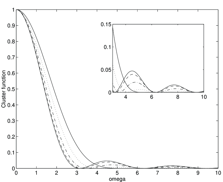
FIG. 1.: The cluster function $Y_{2}$, defined by Eq. (59), against $\tilde{\omega}$ for the parameter values $\tilde{y}_{1}=\tilde{y}_{2}=0$ and $a=0$ (left solid line, the GUE case), $a=0.5$ (dashed line), $a=1.0$ (dot-dashed line), $a=1.5$ (dotted line), and $a=2.0$ (the right solid line, well approximates the Ginibre case)

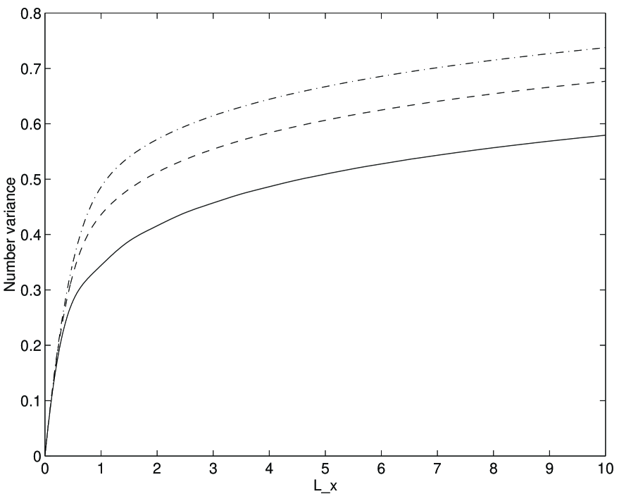
FIG. 2.: The number variance $\Sigma_{2}$, defined by Eq. (62), against $L_{x}$ for the parameter values $a=0$ (solid line, the GUE case), $a=1.5$ (dashed line), and $a=2.0$ (dot-dashed line)

REFERENCES

- [1] Statistical Theory of Spectra: Fluctuations, ed. by C. E. Porter (Academic Press, New York, 1965).
- [2] M. L. Mehta, Random Matrices (Academic Press, San Diego, CA, 1991).
- [3] F. Haake, Quantum Signature of Chaos (Springer-Verlag, Berlin Heidelberg New York, 1991).
- [4] O. Bohigas, in Chaos and Quantum Physics, Proceedings of the Les-Houches Summer School. Session LII, ed. by M.J. Giannoni et.al (North Holland, Amsterdam, 1991), p.91.
- [5] B. L. Altshuler and B. D. Simons, in Mesoscopic Quantum Physics, Proceedings of the Les-Houches Summer School, Session LXI, ed. by E.Akkermans et al.
- [6] C.W.J. Beenakker, Rev.Mod.Phys. 69, 731 (1997)
- [7] T. Guhr, A. Müller-Groeling, and H. A. Weidenmüller, to appear in Rev. Mod. Phys.
- [8] M. Berry, Proc. R. Soc. London, Ser. A 400, 229 (1985).
- [9] E. Bogomolny and J. Keating, Phys.Rev.Lett 77, 1472 (1996).
- [10] B. A. Muzykantsky and D. E. Khmelnitsky JETP Lett. 62, 76 (1995).
- [11] A. Andreev, O. Agam, B. Altshuler and B. D. Simons . Phys.Rev.Lett., 76, 3947 (1996).
- [12] R. Grobe, F. Haake, and H.-J. Sommers, Phys. Rev. Lett. 61, 1899 (1988).
- [13] L. E. Reichl, Z. Y. Chen and M. Millonas Phys. Rev. Lett. 63, 2013 (1989).
- [14] H. Sompolinsky, A. Crisanti, and H.-J. Sommers, Phys. Rev. Lett. 61, 259 (1988); B. Doyon, B. Cessac, M. Quoy, and M. Samuelidis, Int. J. Bifurc. Chaos 3, 279 (1993).
- [15] H.-J. Sommers, A. Crisanti, H. Sompolinsky, and Y. Stein, Phys. Rev. Lett. 60, 1895 (1988).
- [16] V. V. Sokolov and V. G. Zelevinsky, Phys. Lett. B 202, 10 (1988) and Nucl. Phys. A 504, 562 (1989).
- [17] F. Haake, F. Izrailev, N. Lehmann, D. Saher, and H.-J. Sommers, Z. Phys. B 88, 359 (1992); N. Lehmann, D. Saher, V. V. Sokolov, and H.-J. Sommers, Nucl. Phys. A 582, 223 (1995);
- [18] M. Müller, F.-M. Dittes, W. Iskra, and I. Rotter, Phys. Rev. E 52, 5961 (1995).
- [19] Y. V. Fyodorov and H.-J. Sommers, Pis’ma ZhETF 63, 970, (1996) [Engl. tranls. JETP Letters 63, 1026 (1996)].
- [20] Y. V. Fyodorov and H.-J. Sommers, J.Math. Phys., 38, 1918 (1997).
- [21] R. Blumel, Phys. Rev. E, 54, 5420 (1996); V.A. Mandelshtam and H.S. Taylor, J. Chem. Soc. Faraday. Trans., 93,847 (1997) and Phys. Rev. Lett., 78, 3274 (1997).
- [22] J. J. M. Verbaarschot, H. A. Weidenmüller, and M. R. Zirnbauer, Phys. Rep. 129 (1985), 367.
- [23] D. V. Savin and V. V. Sokolov, Phys. Rev. E 56, R4911 (1997); see also the related papers: G.Casati, G.Maspero and D.L.Shepelyansky Phys. Rev. E 56, R6223 (1997); K.Frahm Phys. Rev. E 56, R6237 (1997)
- [24] N. Hatano and D. R. Nelson, Phys. Rev. Lett. 77, 570 (1996) and Phys. Rev. B 56 8651 (1997).
- [25] D. R. Nelson and N.M. Shnerb, e-preprint cond/mat/9708071.
- [26] J. Miller and J. Wang, Phys. Rev. Lett. 76, 1461 (1996); J. Chalker and J. Wang, Phys. Rev. Lett. 79, 1797 (1997)
- [27] K.B. Efetov, Phys.Rev.Lett. 79, 491 (1997); Phys. Rev. B 56, 9630 (1997).
- [28] R.A. Janik M.A. Novak, G. Papp, and I. Zahed, e-preprints cond-mat/9705098 and hep-th/9710103.
- [29] P.W. Brouwer, P.G. Silvestrov and C.W.J. Beenakker Phys.Rev.B 56, 4333 (1997); B.A. Khoruzhenko and I. Ya. Goldscheid, e-preprint cond-mat/9707230.
- [30] E. Brezin and A. Zee, Nucl.Phys.B, 509, 599 (1997); J. Feinberg and A. Zee, e-preprint cond-mat/9710040; A. Zee e-preprint cond-mat/9711114.
- [31] N. M. Shnerb and D. R. Nelson, e-preprint cond-mat 9801111.
- [32] M.A. Stephanov, Phys. Rev. Lett. 76, 4472 (1996); R.A. Janik M.A. Novak, G. Papp, and I. Zahed, Phys. Rev. Lett. 77, 4876 (1996); M. A. Halasz, A. D. Jackson and J. J. M. Verbaarschot, Phys. Lett. B 395, 293 (1997) and Phys. Rev. D, 56, 5140 (1997); M.A. Halasz, J.C.Osborn and J.J.M. Verbaarschot Phys. Rev. D, 56, 7059 (1997)
- [33] M. V. Feigelman and M. A. Skvortsov, Nucl. Phys.B 506, 665 (1997); A. Khare and K. Ray, Phys. Lett. A 230, 139 (1997).
- [34] L. N. Trefethen, Pseudospectra of matrices, in Numerical Analysis, D. F. Griffiths and G. A. Watson (Eds.) (Longman, Harlow, Essex, U.K., 1992), pp. 234 – 266.
- [35] E. Gudowska-Nowak, G. Papp and J. Brickmann Chem.Physics v.220, 125 (1997)
- [36] J. Ginibre, J. Math. Phys. 6, 440 (1965).
- [37] N. Lehmann and H.-J. Sommers, Phys.Rev.Lett. 67, 941 (1991).
- [38] A.Edelman, E.Kostlan and M.Shub J.Am.Math.Soc. v.7 (1994), 247; A. Edelman, J. Multivariate Anal. 60, 203 (1997).
- [39] P.J. Forrester, Phys. Lett. A 169,21 (1992); J. Phys. A: Math. Gen. 26, 1179 (1993).
- [40] G. Oas, Phys. Rev. E 55, 205 (1997).
- [41] Y.V. Fyodorov, B. A. Khoruzhenko and H.-J. Sommers, Phys. Rev. Lett. 79, 557 (1997).
- [42] V. L. Girko Theor. Prob. Appl. 29, 694 (1985) and ibid. 30, 677 (1986).
- [43] Z. D. Bai, Ann. Prob. 25, 494 (1997).
- [44] B. A. Khoruzhenko, J. Phys. A: Math. Gen. 29, L165 (1996).
- [45] Y. V. Fyodorov, B. A. Khoruzhenko and H.-J. Sommers, Physics Letters A 226, 46 (1997);
- [46] R. A. Janik, M. A. Nowak, G. Papp, and I. Zahed Nucl.Phys.B 501, 603 (1997);
- [47] J. Feinberg and A. Zee, Nucl. Phys. B 501, 643 (1997) and ibid 504, 579 (1997).
- [48] M. Kus, F. Haake, D. Zaitsev and A. Huckleberry, J. Phys. A: Math. Gen. 30, 8635 (1997)
- [49] E. P. Wigner, Ann. Math. 62, 548 (1955) and ibid. 67 325 (1958).
- [50] L. A. Pastur, Russ. Math. Surv. 28 3 (1973); see also L.A. Pastur, Annales de l’Institut Henri Poincare. Physique Theoretique 64 325 (1996).
- [51] E. Brezin, C. Itzykson, G. Parisi, and J. Zuber, Commun. Math. Phys. 59, 35 (1978).
- [52] A. Boutet de Monvel, L. A. Pastur, and M. V. Shcherbina, J. Stat. Phys. 79, 585 (1995).
- [53] G. J. Rodgers and A. J. Bray, Phys. Rev. B 37, 3557 (1988).
- [54] A. D. Mirlin, Y. V. Fyodorov, J. Phys. A: Math. Gen. 24, 2273 (1991); Y. V. Fyodorov, A. D. Mirlin, Phys. Rev. Lett. 67, 2049 (1991).
- [55] Y. V. Fyodorov and H.-J. Sommers, Z.Phys.B 99, 123 (1995).
- [56] L. Pastur, Lett. Math. Phys. 25 259 (1992); L. Pastur and M. Shcherbina J. Stat. Phys. 86, 109 (1997).
- [57] E. Brezin, A. Zee, Nucl. Phys. B 402, 613 (1993).
- [58] G. Hackenbroich and H. A. Weidenmüller Phys. Rev. Lett. 74, 4118 (1995).
- [59] Strictly speaking, the form of the correlation function of eigenvalue densities for sparse matrices was shown to be identical to that known for the corresponding Gaussian ensemble provided the average number of non-zero elements in each row exceeds some critical value . The ”threshold” value is nonuniversal. However, direct numerical simulations, see S.Evangelou J.Stat.Phys. v.69 (1992), 361 show that actual value is . Thus even existence of two nonvanishing elements per row already ensure, that the corresponding statistics belongs to the Gaussian universality class.
- [60] J. Ambjorn, J. Jurkiewicz and Y. Makeenko, Phys. Lett. B251, 517 (1990); G. Akemann and J. Ambjorn, J. Phys. A: Math. Gen. 29 L555 (1996).
- [61] A. M. Khorunzhy, B. A. Khoruzhenko and L. A. Pastur J. Phys. A: Math. Gen. 28 L31 (1995) and J. Math. Phys. 37, 5033 (1996); J. D’Anna and A. Zee, Phys. Rev. E 53, 1399 (1996).
- [62] M. Bowick and E. Brezin, Phys. Lett. B 268, 21 (1991).
- [63] Ya. Sinai and A. Soshnikov, private communication.
- [64] K. B. Efetov Supersymmetry in Disorder and Chaos (Cambridge )
- [65] Y. V. Fyodorov, in “Mesosocopic Quantum Physics”, Les Houches Summer School, Session LXI,1994, edited E.Akkermans et al., Elsever Science, 1995, p.493
- [66] A. Pandey and M. L. Mehta, Commun. Math. Phys. 87, 449 (1983).
- [67] A. Altland, K. B. Efetov, S. Iida, J. Phys. A: Math. Gen. 26, 2545 (1993).
- [68] J. H. Wilkinson, The Algebraic Eigenvalue Problem (Clarendon Press, Oxford, 1965).
- [69] Ref. [2], Appendix 35.
- [70] F. Di Francesco, M. Gaudin, C. Itzykson, and F. Lesage, Int. J. Mod. Phys. A 9, 4257 (1994).
- [71] P. J. Forrester and B. Jancovici, Int. J. Mod. Phys. A 11,941 (1997).
- [72] G. Szegö, Orthogonal polynomials, 4th ed. (AMS, Providence, 1975), p. 380.
- [73] I. S. Gradshteyn, I. M. Ryzhik, Table of Integrals, Series, and Products (Academic Press, N.Y. 1980).
- [74] T. Gorin, F.-M. Dittes, M. Müller, I. Rotter and T. H. Seligman , Phys.Rev.E, 56, 2481 (1997).
- [75] Y.V.Fyodorov, M.Titov and H.-J.Sommers , under preparation.