On the Strength of Attractors in a High-dimensional System: Milnor Attractor Network, Robust Global Attraction, and Noise-induced Selection

Abstract

Strength of attractor is studied by the return rate to itself after perturbations, for a multi-attractor state of a globally coupled map. It is found that fragile (Milnor) attractors have a large basin volume at the partially ordered phase. Such dominance of fragile attractors is understood by robustness of global attraction in the phase space. Change of the attractor strength and basin volume against the parameter and size are studied. In the partially ordered phase, the dynamics is often described as Milnor attractor network, which leads to a new interpretation of chaotic itinerancy. Noise-induced selection of fragile attractors is found that has a sharp dependence on the noise amplitude. Relevance of the observed results to neural dynamics and cell differentiation is also discussed.

1 Introduction

Study of a multi-attractor system is important in a variety of physical, chemical, biological, and engineering problems. In a system with many degrees of freedom, coexistence of many attractors is rather common. On the other hand, memory storage to each attractor is often discussed in application of dynamical systems to information processing, where the abundance in attractors is required. In neural dynamics, attribution of attractors to memory is often adopted. In a dynamical system model for cell differentiation, different cell types are often regarded as different attractors in a genetic network.

There are several approaches to a multi-attractor system. Even for a system with low degrees of freedom, dynamical systems studies have revealed (fractal) basin structures and their metamorphose [1]. If the dynamics is of an overdamped type with a function to be minimized, the basin volume is understood from the valley structure of such (energy) function, as shown schematically in Fig.1a). In this case, the dynamics can be understood through the landscape structure, and static representation is possible. Indeed, for a system with many degrees of freedoms, rugged landscape structure has been studied in spin glass, Boolean net, and neural networks, where static aspects of a multi-attractor system are studied [2].

When the system does not have such damping term, further information on the phase space structure is required than the landscape. In a high-dimensional Hamiltonian dynamical system, there are several attempts to make direct “anatomy” [3, 4] of the phase space. Connection path among several ordered states has been studied therein.

If the dynamics is high-dimensional and dissipative, but not of the over-damped relaxation-type, the structure of phase space remains totally unclear. Even for dynamical systems with few degrees, the basin structure is often riddled [5, 6], where the selection of attractors can be regarded almost probabilistic for an initial point distant from the attractors. As the degrees get larger, the study is more difficult, although there are some attempts in cellular automata [8] and in globally coupled map [7, 6].

It is necessary to distinguish the basin volume and the stability of an attractor. The former characterizes how large the area for the attraction is, while the latter gives how strong the attraction is. There can be several possibilities on the definition of stability of an attractor. In §2 we will introduce a few of them, and discuss one of them in detail.

As a specific example of a multi-attractor system, we choose a globally coupled map (GCM), where the characterization and coding of attractors are rather straightforward. In §3, bifurcation of several attractors in GCM is surveyed, with the emphasis on the change of basin volume.

In §4, the stability of attractors in GCM is characterized using the measures introduced in §2. It is found that there is a class of attractors that globally attracts orbits, but whose orbits are kicked away from them by any small perturbation. Such attractor without the stability is called Milnor attractor[9, 10]. By adopting the quantifiers for the stability introduced in §2, it is shown that global attraction is rather robust in contrast with local stability. Appearance of Milnor attractors is due to the discrepancy between the global attraction and the local stability. In §5, it is shown that Milnor attractors are quite common in the partially ordered phase in GCM. Such dominance of Milnor attractors is preserved with the increase of system size, and is a general feature in a system with many degrees of freedom, as is demonstrated in §6.

By perturbing an attractor with a small noise, orbits can be switched to a different attractor. Through this switch, connectivity matrix among attractors is defined depending on the input noise. In §7 this connectivity is studied. In particular, in the partially ordered phase, the dynamics is shown to be represented by connection network among Milnor attractors. This dynamics over Milnor attractors reminds us of the chaotic itinerancy, previously found as the itinerant dynamics over attractor ruins. In §8, the chaotic itinerancy is re-interpreted as Milnor attractor networks.

Existence of attractors with weak stability may lead us to suspect that the orbits might not be attracted to them in the presence of noise. In §9, we have studied the rate of attraction to each attractor in the presence of noise. In contrary to our naive expectation, weak, or even Milnor, attractors may attract more orbits in the presence of noise. This mechanism is discussed in relation with the global attraction in the phase space. Complicated dependence of the attraction rate on the noise strength is found, which reflects the complex connection among attractors.

Relevance of our observation to biological networks is given in §10, focusing on dynamic information processing in neural dynamics, and developmental process of cell society. Summary and discussion are given in §11 (see also ref.[11] for rapid communication).

Figure 1: Schematic representation of strength of an attractor: a) overdamped motion of $x$ in a potential $U(x)$ b) dynamics without a potential

2 Stability of Attractors

It is natural to define stability of an attractor in relation with the degree of return of an orbit to the attractor when it is perturbed. Now there are choices on the measure of return, and the way how to perturb the orbit.

Let us start with a trivial example with over-damped motion in a ’potential’ (see Fig.1). In this case, the stability of fixed points at the bottom of each valley can be discussed by the depth of a hill $H$, and its basin size $W_{1}+W_{2}$. Consider two extreme cases, one is stability against a one-shot noise and the other for the stability under continuous presence of noise. The stability in the former case is related with the minimum of $(W_{1},W_{2})$, since the orbit perturbed to $x_{0}+\delta$ remains within the same valley if $\delta<$minimum of $(W_{1},W_{2})$ (see Fig.1). On the other hand, the dynamic stability in the presence of noise is often characterized by the height $H$, as is typically expressed by the Kramers formula $exp(-H/(kT))$ for the transition probability from one valley to another when the system is under a Gaussian white (or a similar) noise with $kT$ corresponding to the noise strength.

Here we aim at generalizing the stability to a high-dimensional dissipative case, without a potential. To characterize an attractor, we discuss the basin volume, and measures of static and dynamic stability.

The basin volume of an attractor is estimated as the ratio of initial points that are attracted to it, by choosing them randomly. Even though the basin is generally not a smoothly connected object, with its fractal or riddled basin structure, this estimate still works as an effective means.

Although the basin volume ($W_{1}+W_{2}$) and the static stability (minimum of $(W_{1},W_{2})$) are highly related in the above one-dimensional static potential case, they are in general independent. Even if the basin is smooth, the static stability is distinguishable from a basin volume. As a simple illustration consider the case schematically given by Fig.1b). As long as a one-shot perturbation is smaller than $\sigma_{c}$, the orbit returns to the attractor after the perturbation. For this simple case, the stability is related with the minimal distance between the attractor and its basin boundary, in contrast with the basin volume.

Although there can be several possible ways for the definition of (static) stability, it is defined as follows here: Perturb an orbit on an attractor at one time, and leave the system evolve according to its dynamics (without perturbation), and check if the orbit comes back to it, after transients are decayed. The static stability is defined from a measure of the degree of return to the original attractor.

To be specific, we define the return probability as follows. Consider an $N$-dimensional dynamical system for $x(i)$ ($i=1,\cdots,N$). Take an orbital point $x(i)$ on an attractor, and perturb the orbit by $\sigma$, i.e., $x(i)+\sigma\times rnd(i)$, as $rnd(i)$ a random number taken from $[-.5,.5]$. By taking this perturbed point, evolve the system according to the dynamics (without the noise term), and check if the orbit reruns to the original attractor or not. Repeat this trial a large number of times, and define the return rate $P(\sigma)$ as the ratio of returns to the number of all trials. $P(\sigma)$ characterizes how paths to other attractors are opened as the orbit is perturbed from the attractor. The smallest $\sigma$ ($\sigma_{c}$) such that $P(\sigma)$ is less than 1 gives an estimate for the strength of an attractor. In the previous examples, $\sigma_{c}$ gives the minimal distance between the attractor and the basin boundary.

Later we will see that there are “attractors” with $\sigma_{c}=0$. Although such “attractors” are not asymptotically stable, we will see that a large number of initial points is attracted to them at some parameter regime. For such attractors, $P(+0)\equiv\lim_{\sigma\rightarrow 0}P(\sigma)$ gives another measure for the strength.

Of course, it is often important to discuss the form of $P(\sigma)$ itself, which is relevant to characterize global attraction in the phase space. As another estimate for the strength, we define $\sigma_{m}$ as the half-return threshold, i.e., the smallest $\sigma$ such that $P(\sigma)$ is less than 0.5.

Besides the stability, it is also interesting to discuss connection among attractors. Using the above perturbation, one can define the probability transition matrix $T(i,j;\sigma)$ from one attractor $i$ to another attractor $j$. ($P_{i}(\sigma)=T(i,i;\sigma)$). With this transition matrix, ‘connectivity’ among attractors in the presence of noise, or ‘distance’ among attractors in its rough sense, can be discussed.

On the other hand, the dynamic stability can be discussed as the residence probability to each attractor in the presence of noise. However, it is in general, not possible, to check precisely if the orbit stays at an attractor in the presence of noise. One possible way to define the dynamic stability is the use of the return rate $P(\sigma)$ and the transition matrix $T(i,j;\sigma)$ after the noise is added over long enough time steps continuously. Instead of it, we check to which attractor the orbit is settled after the noise is added for (long enough) time steps. The rate of attraction $V(\sigma)$ is defined as a function of noise strength $\sigma$. The value $V(\sigma)-V(0)$ for an attractor gives a measure of the net flow to the attractor from others, in the presence of noise.

Some quantifiers and terms adopted in the present paper are summarized in Table I.

Table I:Summary of quantifiers and terms adopted in the present paper (see text for details)

Basin Volume	the ratio of initial points attracted to the attractor,
Ratio $V$	to all the randomly chosen initial points
Return Rate	Rate of points that return to the original attractor
$P(\sigma)$	after a random perturbation with the size $\sigma$ is applied
$\sigma_{c}$ (strength)	the minimum strength of perturbation that leads to $P(\sigma)<1$
$P(+0)$	characterizes the asymptotic stability
robust attractor	an attractor with $\sigma_{c}>0$
Milnor attractor	an attractor with $\sigma_{c}=0$, i.e., $P(+0)<1$
fragile attractor	an attractor with $P(+0)<1$ but close to 1
pseudo attractor	an attractor with $P(+0)<<1$, to be regarded as a transient
	state that is trapped as an artifact of digital computation
probability transition	rate of transition form attractor $i$ to $j$ with
matrix $T(i,j,\sigma)$	the perturbation $\sigma$
basin volume $V(\sigma)$ in	ratio of initial points attracted to the attractor
the presence of noise	with the random noise over initial time steps

3 Revisit to partially ordered phase in GCM

As an example of high-dimensional dynamical systems with potentiality of many attractors, we adopt the globally coupled map (GCM) [7] given by

$$x_{n+1}(i)=(1-\epsilon)f(x_{n}(i))+\frac{\epsilon}{N}\sum_{j=1}^{N}f(x_{n}(j)),$$ (1)

where $n$ is a discrete time step and $i$ is the index for elements ($i=1,2,\cdots,N$ = system size). Here we choose the logistic map $f(x)=1-ax^{2}$ as the local element in eq.(1), as it has been investigated as a standard model for a high-dimensional dynamical system. Throughout the paper we fix the parameter $\epsilon=.1$. In the model, attractors are known to be coded by clustering, that is the partition of $N$ elements into mutually synchronized clusters, i.e., a set of elements in which $x(i)=x(j)$ [7]. Attractors in GCM are classified by the number of synchronized clusters $k$ and the number of elements for each cluster $N_{k}$. Each attractor is coded by the clustering condition $[N_{1}(\geq),N_{2}(\geq),\cdots,(\geq)N_{k})]$. Due to the symmetry, there are at least $\frac{N!}{\prod_{i=1}^{k}N_{i}!}\prod_{oversetsofN_{i}=N_{j}}\frac{1}{m_{\ell}!}$ attractors for each clustering condition, where $m_{\ell}$ is the number of clusters with the same value of $N_{j}$. This estimate is based on the assumption that the cluster with the same number of elements is indistinguishable due to the symmetry. For example the attractor with $[2,2,2,2,2]$ has 945-fold degeneracy.

This number of attractors can be under-estimated, since different attractors can exist for the same partition. For example, period-2 type band motion sometimes remains. Although elements are desynchronized, they keep the relation on the band motion ( see Fig.2 and Fig.3 for some examples of such coexisting attractors.). The attractors in Fig.2 can be classified by adopting band-splitting instead of clustering. The attractor of Fig 2a is given by (2-band;(5:5)) while that of Fig.2b by (2-band(7:3)). For the attractors with the clustering of, say [3,1,1,..1], there can be a few attractors with a different partition into two bands. In Fig.3a, elements split into two bands with 4 elements clustered into [3,1] and 6 elements mutually desynchronized, denoted by the band (4[3,1],6[1,1,…,1]). Another attractor with the same clustering [3,1,..,1] coexists at $a=1.65$ (and $\epsilon=0.1$), which has a band splitting to 3 and 7 elements, where the former are synchronized and the latter desynchronized. Since for most parameters one-to-one correspondence between clustering and an attractor holds ( at least for that with a large enough basin volume to be detected numerically), and the classification both with the band and clusterings is complicated, we distinguish the attractors only by the clustering, unless the use of both is necessary.

Figure 2: Overlaid time series of $x_{n}(i)$ of the attractor with the clustering [1….1], accompanied by the time series of the mean field. $a=1.66,\epsilon=.1,$ and $N=10$. Two examples. (a) the band splitting with 5:5 (b) band splitting with 7:3.

Figure 3: Overlaid time series of $x_{n}(i)$ of the attractor with the clustering [3,1…,1], accompanied by the time series of the mean field. $a=1.65,\epsilon=.1,N=10$. Three examples. (a) the band splitting with 4:6 (b) band splitting with 7:3.

With the increase of nonlinearity $a$ or decrease of coupling $\epsilon$, the following phases appear successively after the collapse of a completely synchronized state; (i) Coherent phase: Only a coherent attractor ($k=1$) exists. (ii) Ordered (O) phase: All attractors consist of few ($k=o(N)$) clusters. (iii) Partially ordered (PO) phase: Attractors with a variety of clusterings coexist, while most of them have many clusters ($k=O(N)$). (vi) Turbulent phase: Elements are completely desynchronized, and all attractors have $N$ clusters.

In the ordered and partially ordered phases, there exists a variety of attractors depending on the partition. In Fig.4, basin volumes for attractors with different clusterings are plotted, where the decimal representation of the clusterings $[N_{1}N_{2}\cdots N_{k}]$ is adopted for each attractor. Successive appearance of attractors with the cluster numbers 2,3, 4 $\cdots$ proceeds at the ordered phase, and attractors with a large number of clusters are dominant at the PO phase.

For a system with a larger number of elements, enumeration of all attractors by $[N_{1}N_{2}\cdots N_{k}]$ is almost impossible. Hence it is necessary to introduce some other simple measures. The simplest measure is just the number of attractors, which is enhanced at the border between O and PO phases. A better quantifier to incorporate with the clustering is the ratio that two elements fall into the same cluster defined by $Y\equiv\sum_{j}(N_{j}/N)^{2}$ [12]. See Fig.5 for the parameter dependence of the basin volume rate to each $Y$ value. Note that $Y$ is close to 1/2 for a ( typical or evenly partitioned) 2-cluster attractor, 1/3 for a typical 3-cluster attractor, and so forth. Successive appearance of attractors with a larger number of clusters is seen in Fig. 5.

The ‘partition complexity’ is defined in [12] as the fluctuation of $Y$ over initial conditions. It is found that this fluctuation remains finite in the thermodynamic limit at the PO phase, whose value is enhanced at the border between O and PO phases.

Another simple way is the use of entropy-like function from the cluster probability. The probability $p^{clust}(i)$ is defined as the basin ratio of attractors with the cluster number $i$. The function $-\sum_{j}p^{clust}(j)lnp^{clust}(j)$ has a peak again at the boundary between O and PO phases [13]. Hence measures to characterize the variety of attractors defined from the basin volume ratio has a peak at the PO phase (precisely speaking at the border between O and PO), while correspondence of the PO phase with the spin glass has been emphasized [12, 13].

Figure 4: Change of the partition code for existing attractors, with the change of $a$. The vertical axis gives the number $[N_{1}N_{2}\cdots N_{k}]$. For example the largest partition code corresponds to 1111111111, and the smallest one is 55. By taking 10000 initial conditions, and iterating our dynamics over 100000 steps, we have checked on which attractor the orbit falls. Hereafter the basin volume rate is computed with this procedure, and is measured as the sum of all rates over the attractors with the same partition $[N_{1},..N_{k}]$, unless otherwise mentioned. The rate of initial conditions leading to such partition is plotted as different marks. $\triangle$( $>50$%),$\times$ ($>10$%), $\Box$($>5$%), $+$($>1$%), and $\Diamond$($>.1$%).

Figure 5: The basin for each $Y$ value, with the change of $a$. The rate of initial conditions leading to such value of $Y$ is plotted as different marks. $\triangle$( $>50$%),$\times$ ($>10$%), $\Box$($>5$%), $+$($>1$%), and $\Diamond$($>.1$%). See text for the definition of $Y$.

Another measure for the split of elements is given by the split exponent $\lambda_{spl}$ defined by

$$\lambda_{spl}=(1/N)\sum_{j}\lambda_{spl}^{j}=(1/N)\sum_{j}log|(1-\epsilon)f^{\prime}(x(j))|$$ (2)

where the exponent gives a measure for the average split rate of two elements taking close values[14].

As is shown in Fig.6, the basin volume of the attractors with $\lambda_{spl}\approx 0$ increases around the onset of partially ordered phase, while the completely desynchronized phase appears with the further increase of $a$. Attractors with $\lambda_{spl}>0$ start to appear around $a\approx 1.61$, which corresponds to the appearance of attractors with many clusters, while the average of $\lambda_{spl}$ over initial conditions starts to be positive at the PO phase around $a\approx 1.66$.

Figure 6: Basin volume for attractors with $\lambda_{spl}$, as $a$ is changed. The rate of initial conditions leading to such value of $\lambda_{spl}$ with the bin size 0.01 is plotted as different marks. $\triangle$( $>50$%),$\times$ ($>10$%), $\Box$($>5$%), $+$($>1$%), and $\Diamond$($>.1$%). The average over 10000 initial conditions is also plotted as a line.

Before studying the attractor strength, let us discuss the bifurcation of the GCM in a more detail, adopting the basin volume change. In Fig.7, the basin volume rates to attractors of given partitions are plotted for $N=10$. As the parameter $a$ is increased, attractors with more clusters appear successively. Two-cluster attractors disappear around $a\approx 1.58$, three clusters at $a\approx 1.6$, 4, 5, and 6 clusters around 1.65. Roughly speaking, for $a>1.65$ the attractors with the type of $[k,1,1,1,\cdots]$ are dominant as to the basin volume.

Figure 7: Change of the basin volume rates with the parameter $a$. $N=10$. (a) the basin volume rates for two-cluster attractors. (b) the basin volume rates for three-cluster attractors. (c) the basin volume rates for attractors with the partition $[\ell,1,\cdots,1]$.

At the ordered phase with smaller $a$ ( e.g., $a<1.65$ for $\epsilon=.1$) two- and three-cluster attractors are dominant. Two-cluster attractors lose their stability successively from biased partitions (e.g. [9,1],[8,2],[7,3],…). Note that there are several ‘cliffs’ in the basin rate of a two-cluster attractor ( see e.g., the basin rate for [5,5] attractors). Indeed the cliffs are seen when an attractor with a split cluster from it has a larger basin volume. For example, the cliff around $a\approx 1.55$ for a [5,5] attractor is due to the increase of the basin volume of the [5,4,1] attractor. By some change in the phase space structure, new paths to [5,4,1] attractors are opened, by which some orbits previously attracted to [5,5] attractors are attracted to [5,4,1].

As the number of clusters increases, more paths are opened or closed with the parameter change, which leads to complicated bifurcation structures for attractors with 4, 5, and more clusters. Among them, a clear structure is seen as successive appearance of $[\ell,1,,,1]$ attractors with decreasing $\ell$, when $a$ is increased from 1.5, as shown in Fig. 7c).

4 Existence of Fragile attractors and Stability of Global attraction

Now we study how the stability of attractors change, by using the return probability $P(\sigma)$, defined in §2. See Fig.8 for examples of $P(\sigma)$ for some attractors. There are two types of behaviors in $P(\sigma)$. The first one is that with $P(\sigma)=1$ up to some threshold $\sigma>0$. Indeed, this behavior is expected for an asymptotically stable attractor. In this case, the ‘strength’ of attractor is measured by defining $\sigma_{c}$ as the smallest $\sigma$ such that $P(\sigma)<1$, as mentioned.

In contrast with our naive expectation from the concept of an attractor, there are some ‘attractors’ with $\sigma_{c}=0$, i.e., $P(+0)\equiv\lim_{\delta\rightarrow 0}P(\delta)<1$. If $\sigma_{c}=0$ holds for a given state, it cannot be an “attractor” in the sense with asymptotic stability, since some tiny perturbations kick the orbit out of the “attractor”. The attractors with $\sigma_{c}=0$ are called Milnor attractors. In other words, Milnor attractor is defined as an attractor that is unstable by some perturbations of arbitrarily small size, but globally attracts orbital points with a finite Lebesgue measure. Since it is not asymptotically stable, one might, at first sight, think that it is rather special, and appear only at a critical point like the crisis point in the logistic map[9]. Recent discovery of riddled basin attractors, however, leads us to expect that such attractors may not be so special[1, 6]. One of the claims in the present paper is that they are rather common at a high-dimensional dynamical system, in particular at the partially ordered phase.

Figure 8: $P(\sigma)$ for several attractors for $a=1.64$, and $N=10$. For all the figures, we have 10000 initial conditions randomly chosen over $[-1,1]$ for each parameter, to make samplings. $P(\sigma$) is estimated by sampling over 1000 possible perturbations for each $\sigma$. We often use the abbreviated notation like $31^{7}$ for $[3,1,1,1,1,1,1,1]$. Plotted are robust attractors [32221] (with the basin volume rate $V\approx 6.3\%$ and $\sigma_{c}\approx.01$) and [3322] (with $V\approx 15$% and $\sigma_{c}\approx$.0012), fragile attractors [31111111] (with $V\approx 42$%), [22111111] (with $V\approx 29$ %), and pseudo attractors [4321] (with $V\approx.2$%) and [4111111] (with $V\approx 4.8\%$).

Milnor attractors of our model are rather well separated into two types; one with $P(+0)$ close to 1, the other with $P(+0)$ close to 0 (see Fig.8). For the former type, which we call “fragile” attractor, $P(\sigma)$ is close to 1 up to some perturbation strength $\sigma$ and decreases for larger $\sigma$. The other type with much smaller $P(+0)$, to be called ‘pseudo-attractor’, shows increase in $P(\sigma)$ for larger $\sigma$. (See also Table I in §2 for the terminology adopted in the present paper). One relevant index to characterize the strength of these attractors is given by $P(+0)$.

The above distinction between the two types of Milnor attractors may look mathematically ill-defined. In our simulations, however, the values of $P(+0)$ are rather well separated, either into $>.5$ or $<.1$. Practically speaking, we call attractors with $0.5<P(+0)<1$ as “fragile”, while those with $P(+0)<0.5$ are pseudo-attractors. Indeed, the reason why we call the latter as ‘pseudo’ is that this attraction is thought to be due to a finite precision in computation. In ref.[14], we have reported that iterations of (1) with any finite precision can lead to a pseudo-attractor due to artificial synchronization (see also [15]). If the split exponent, measured over some time steps, remains negative for long enough time, then two elements may be synchronized down to its smallest bit in the computer. Then, even if they are supposed to desynchronize later, they cannot do in a digital computer. Indeed, the ‘pseudo-attractors’ in our simulation have very small basin ratio, which can be affected by a way of computation. Hence we mostly focus on the stable and fragile attractors later.

As another measure for the stability of an attractor against a larger noise, we also use ‘half-decay threshold’ $\sigma_{m}$ defined as the smallest $\sigma$ such that $P(\sigma)<0.5$. For a fragile attractor $\sigma_{m}$ is positive, while it is zero for a pseudo-attractor.

It is interesting to note that $P(\sigma)$ sometimes increases with the increase of $\sigma$ (see Fig.9). Such increase is generally seen in weak attractors, and in Milnor attractors. As a simple example in the ordered phase, take a two-cluster attractor. At $a=1.5$, we have attractors with the clusterings [5,5],[6,4],[7,3],and [8,2]. At this parameter regime, the [5,5] attractor has the largest $\sigma_{c}$, which decreases as the partition is biased. $P(\sigma)$ for the [5,5] attractor decreases monotonically, while those for [7,3],[8,2] attractors have a double humped structure. After $P(\sigma)$ approaches 0, it shows an increase for larger $\sigma$, and has an extremum around $\sigma\approx 0.5$. Indeed $P(\sigma)$ for large $\sigma$ is smallest for the [5,5] attractor, and gets larger as the partition is biased. This is an example showing that a weaker attractor can have a larger global attraction, which indeed is seen generally in our system.

Figure 9: $P(\sigma)$ for two-cluster attractors, with the clustering [5,5], [6,4] [7,3], and [8,2].

Extreme examples of global attraction are seen in pseudo- and fragile attractors. In the pseudo-attractor, $P(\sigma)$ increases slightly as $\sigma$ is increased from 0. In this sense, there are some points attracted globally to the pseudo-attractor, although there always exists a path going out of it. In Fig.10 a)b), we have plotted such examples.

In Fig.10a), we have plotted the change of $P(\sigma)$ for the [2,2,1,1,..,1] attractor with the increase of the parameter $a$, as it changes from robust, to fragile, and then to pseudo attractors. One can clearly see that the function $P(\sigma)$ is not much changed for large $\sigma$, although the structure at smaller $\sigma$ is largely changed.

Another example with a smaller number of clusters is given by Fig.10b), where the change of $P(\sigma)$ for [5,3,2] attractor is plotted. Although $P(0)$ changes sensitively on the parameter $a$ here, and the attractor changes from fragile, pseudo, and robust ones. Again, the global attraction is rather robust in contrast with the change of stability near the attractor.

This discrepancy between global attraction and local stability, as well as the stability of global attraction against the parameter change, will be important later. It should be noted that the basin volume reflects global attraction more, which leads to the existence of weak or fragile attractors with a large basin volume. Indeed, $P(0)$ that characterizes the local attraction often changes sensitively on the parameter $a$, but the basin volume changes smoothly as will be shown in the next section.

Figure 10: a) $P(\sigma)$ for [2,1,1,1,…1] with the change of $a$ for $a=1,6,1.62,\cdots 1.63$. The attractor is robust for $a=1.6$ and 1.61, fragile for 1.62, and pseudo for 1.63. The inlet is the expansion near $P(\sigma)=1$. b) $P(\sigma)$ for [5,3,2] with the change of $a$. The attractor is fragile ($a=1.6$), pseudo (1.61) and robust (1.62).

The strength and basin volume of attractors are not necessarily correlated. It should be noted that such fragile attractors can have a large basin volume. Often $\sigma_{c}$ is small, (i.e.,the attractor is weak) even if the basin volume is large, when the orbit is located near the basin boundary. In Fig.11, we have plotted $\sigma_{c}$ versus basin volume rate $V$. Points from $a=1.57,58,\cdots 1.62$ are overlaid with different marks. Roughly speaking, there are three groups of attractors. One of them keeps some relationship between the two, ($V\propto\sigma_{c}^{m}$ with $m\approx(1\sim 3)$), while two other groups are deviated from this trend. One is a group of fragile attractors with $\sigma_{c}=0$ with a relatively large basin volume and the other is a strong attractor ($\sigma_{c}\stackrel{{\scriptstyle>}}{{\approx}}0.005$) with relatively smaller basin volume.

Figure 11: Strength $\sigma_{c}$ versus basin volume. $\sigma_{c}$ is estimated from $P(\sigma)$ measured by changing $\sigma$ 20% successively from $10^{-5}$. The points at $\sigma_{c}=10^{-5}$ just represent that $\sigma_{c}<10^{-5}$. For Fig.11-13, we have estimated $\sigma_{c}$ from 100 possible perturbations: $\sigma_{c}$ is regarded to be less than the value of $\sigma$ adopted in the run, as long as all of 100 trials result in the return to the original attractor.

It may be useful to note some relationship between the basin volume and the strength by taking a schematic example. If the basin is given by a hyper-ellipsoid with the radii $r_{1}(\leq)$,$r_{2}(\leq)$,$\cdots$,$(\leq)r_{N}$, and the attractor is localized around the center of it, the strength $\sigma_{c}$ is given by the minimum of $r_{j}$ (i.e., $r_{1}$). In our clustered attractors, there is often some degeneracy of $r_{j}$ due to the symmetry. If few $r_{j}$’s ($j\leq m$) are relevant to $\sigma_{c}$ ($r_{j}\approx\sigma_{c}$) while others remain large and insensitive to the choice of attractors, we could roughly estimate $V\propto\sigma_{c}^{m}\times O(1)$. In this context the points on the same power-law correspond to attractors with similar basin shapes.

5 Dominance of Milnor Attractors at the PO phase

Figure 12: Dependence of $\sigma_{c}$ on the parameter $a$, for $N=100$. By measuring $\sigma_{c}$ for attractors fallen from $10^{4}$ random initial conditions, a histogram of $log_{10}\sigma_{c}$ is constructed with a bin size 0.1. The number of initial conditions leading to $log_{10}\sigma_{c}$ within the bin is plotted as different marks. $\triangle$( $>50$%),$\times$ ( $>10$%), $\Box$($>5$%), $+$($>1$%), and $\Diamond$($>.1$%). For all figures we have estimated $\sigma_{c}$ following the procedure given in the caption of Fig.11. The points at $\sigma_{c}<10^{-4}$ just represent that $\sigma_{c}<10^{-4}$.

Figure 13: Average strength $\sigma_{c}$ plotted as a function of $a$. The basin volume of each attractor is estimated as the rate of initial points leading to the attractor, divided by the degeneracy. The average is taken over $10^{4}$ random initial conditions. For $N=10$, the strength is measured by increasing $a$ by 0.001, while for $N=50$ and $N=100$ it is measured by the increment 0.01.

Here we study parameter dependence of the attractor strength to see the dominance of attractors in the PO phase. In Fig.12, we have plotted the strength $\sigma_{c}$ of attractors with the change of $a$. We note the decrease of strength at the PO phase. The average of attractor strengths (over random initial configurations) is plotted in Fig.13. The results are summarized as follows (by fixing the parameter $\epsilon$ at 0.1).

(1) $a\stackrel{{\scriptstyle<}}{{\approx}}1.62$[16] ( ordered phase) Robust attractors with 2 or 3 clusters take up a large basin volume, although a robust attractor with $[1,1,\cdots,1]$ with a single band (with a synchronized band motion) may also coexist. No fragile attractors exist.

(2) $a\stackrel{{\scriptstyle<}}{{\approx}}1.65$ ( complex ordered (CO) region in the ordered phase): There are a variety of attractors with different partitions, although the number of clusters is not huge ( in other words, it is o(N) for large $N$). The number of attractors increases towards the border between CO and PO phases, and the basin volume for each attractor is small[11]. Some attractors start to have positive $\lambda_{spl}$. There appears fragile attractors with a large basin volume, besides strong attractors with a small number of clusters.

(3) $a\stackrel{{\scriptstyle<}}{{\approx}}1.68$ ( partially ordered phase): The split exponent $<\lambda_{spl}>$ averaged over initial conditions starts to be positive at this phase. In other words, the tendency to split elements overcomes the synchronization. Thus the number of clusters is typically large ($O(N)$), while the basin volume for each attractor is larger than the case (2). For example, for $N=10$, the attractors with $[2,2,1\cdots,1]$ with $P(+0)=.72$ has 60% basin volume, and that with $[1,1,\cdots,1]$ with $P(+0)=.99$ has 36%, at $a=1.661$. For $N=10$, all detected attractors are Milnor attractors, around $a=1.66$.

(4) At $a\stackrel{{\scriptstyle>}}{{\approx}}1.69$, a single desynchronized attractor takes up all basin volume.

What causes the dominance of fragile attractors at the PO phase? First we note that global attraction in the phase space is still kept, when an attractor loses its stability. This is expected by the fact that $P(\sigma)$ at large $\sigma$ keeps a rather large value, even when $P(+0)$ starts to be smaller than unity. Recall that $P(\sigma)$ for large $\sigma$ is not so much changed, while the change from robust, fragile, to pseudo attractors proceeds. (see Fig.10).

This robustness of global attraction is a key to the understanding of the dominance of Milnor attractors at the PO phase. Note there are a large number of attractors at the border between O (CO) and PO. Most of them lose the stability at the CO and PO phases successively. When the stability of an attractor is lost, there appears a set of points in the vicinity of the attractor, that are kicked out of it through the temporal evolution, while the global attraction still remains. This is a reason why fragile attractors are dominant around the PO phase. In Fig.14, we have plotted the sum of basin volume rates for all the Milnor attractors. Dominance of Milnor (fragile) attractors is clearly seen. It is also interesting to note that the basin rate for Milnor attractors sensitively depends on the parameter $a$.

Figure 14: The basin volume ratio of Milnor attractors with the change of $a$. For each $a$, we take 1000 initial conditions, and iterate the dynamics over 100000 steps to get an attractor. We check if the orbit returns to the original attractor, by perturbing each attractor by $\sigma=10^{-7}$ over 100 trails. If the orbit does not return at least for one of the trails, the attractor is counted as a Milnor one. For $N=10$, the ratio is measured for $1.5<a<1.7$ with the increment 0.001, while for larger sizes it is measured only for $1.62<a<1.7$ with the increment 0.01.

The results imply that attractors are often near the crisis point[17] and lose or gain the stability at many parameter values in the PO phase. Furthermore, the stability of an attractor often shows sensitive dependence on the parameter. It is interesting to see how $P(+0)$ and basin volume change with the parameter $a$, when an attractor loses asymptotic stability. In Fig.15 we have plotted the change of the two quantifiers for the attractors with $[3,1....,1]$, $[2,1,...,1]$, $[2,2,1,..,1]$ and $[1,1,...,1]$. In Fig.15a), the basin volume has a peak when the attractor loses the stability and then decreases slowly as $P(0)$ gets smaller than unity, and the attractor becomes a Milnor one. Although the local attraction gets weaker as $P(+0)$ is smaller than 1, the global attraction remains. Furthermore, the basin volume often has a peak around the parameter value of the change of stability (i.e., where $P(+0)$ starts to be less than 1), which is rather commonly observed for several attractors. Indeed, slight increase in the basin volume is seen for the attractors with $[2,1,...,1]$ and $[1,1,...,1]$ when $P(0)$ gets smaller than 1. It is also noted that $P(0)$ often shows sensitive dependence on $a$, when it is smaller than 1. The attractor $[2,2,1,..,1]$, with a relatively large basin volume, is often fragile, around $1.63<a<1.67$.

Figure 15: Change of the strength and basin volume rate with the increase of $a$ by 0.001. For each attractor, the orbit is perturbed by $\sigma=10^{-7}$ over 1000 trails, to get the return rate $P(+0)$, while the basin volume is measured from $10^{4}$ initial conditions. If none of the initial conditions leads to the attractor, the strength is not plotted (while the basin volume is plotted as 0). (a) the attractor [3,1,..,1] with the band splitting (3:7) (b) the attractor [2,2,1,..,1] (c) the attractor [2,1,…,1] (d) the attractors [1,1,..,1] with the band splitting (10:0) (written as $1^{10}-0$), (7:3) ( $1^{10}-3$), (6:4) ( $1^{10}-4$), and (5:5) ( $1^{10}-5$). ”S” shows the strength $P(0)$, ”B” the basin volume ratio.

6 Size Dependence

The dominance of fragile attractors is preserved as $N$ is increased, as shown in Fig.14[16], while $<\sigma_{c}>$, the average of $\sigma_{c}$ over initial conditions is also shown in Fig.12. Roughly speaking, $<\sigma_{c}>$ seems to be smaller with the increase of $N$ at PO phase, although the size dependence of $<\sigma_{c}>$ is irregular. As is discussed and seen in these figures, the PO phase shifts to a higher value of $a$. Except this shift, the dominance of fragile attractors is rather common, and preserved for large $N$.

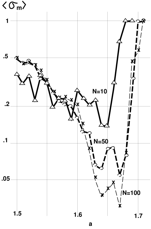
Figure 16: Size dependence of $<\sigma_{m}>$. The value $\sigma_{m}$ is estimated from $P(\sigma)$, measured by changing $\sigma$ as $10^{-4+j/4}$ for ($j=0,1,\cdots,16$), by taking 1000 possible perturbations, while, for $N=50$ and $N=100$, we have made only 100 possible perturbations.

On the other hand, we have also plotted the average of $\sigma_{m}$ in Fig.16, with the increase of the size $N$. The average of $<\sigma_{m}>$ decreases with $N$, which is related with the escape paths from attractors. To consider the paths, let us discuss the size dependence of $P(\sigma)$ for each attractor.

With the increase of $N$, the strengths $\sigma_{c}$ for attractors with a proportional partition (e.g., $[6,4]$ for $N=10$ versus $[60,40]$ for $N=100$) approaches a size independent value, while the value of $\sigma_{m}$ decrease monotonically. In Fig.17, $P(\sigma)$ for the two-cluster attractors with equal partition (i.e., [5,5] for $N=10$ and [50,50] for $N=100$) are plotted with the increase of the size $N$. The strength $\sigma_{c}$ is invariant, while the slope in the decay of $P(\sigma)$ gets larger with the increase of $N$. The latter is due to the increase of the dimension of the path out of the attractor, since the decrease rate in $P(\sigma)$ for $\sigma>\sigma_{c}$ reflects the volume of the path.

The dimension of the exit path is highly correlated with the number of elements in synchronized clusters. For example, take an attractor with the clustering [3,1,1,..,1]. If the perturbation destroys the synchronization of the first three elements, the orbit is easily kicked out of the attractor, while stronger perturbation for the desynchronized 7 elements is required to kick the orbit. Thus the relevant dimension of the exit path is less than $2(=3-1)$. Roughly speaking, the dimension of the exit path for small $\sigma$ is correlated with $\sum_{j}(N_{j}-1)$. The decrease in $<\sigma_{m}>$ at the CO and PO phases (as in Fig. 16) is due to increase of dimensionality in paths out of the attractors.

In Fig.18, we have plotted $P(\sigma)$ for many-cluster attractors for $N=50$ and $N=100$. Here (for $a=1.65$ at the CO phase), two groups exist. One has a larger $\sigma_{c}$, and positive $\lambda_{spl}$, and a larger number of clusters with the clustering $[N_{1},N_{2},1,1,...,1]$ ( e.g., [12,10,1.,,1] for $N=50$ and $[22,21,1,...,1]$ for $N=100$). For this group, not only the threshold $\sigma_{c}$ but also the decay slope of $P(\sigma)$ near $\sigma\stackrel{{\scriptstyle>}}{{\approx}}\sigma_{c}$ does not change so much with the size $N$. The other group has a smaller or null $\sigma_{c}$, negative $\lambda_{spl}$, and a fewer number of clusters. Examples are [12,12,9,8,6,2,1] for $N=50$ and [29,22,21,19,6,2,1] for $N=100$. Although $\sigma_{c}$ is not changed significantly, the decay in $P(\sigma)$ is faster with the increase of $N$, as in the case for the two-cluster attractors.

In general, the path of exits gets larger with the size $N$ for a few number of clusters ($k=o(N)$). The decay in $P(\sigma)$ with $\sigma$ is faster. On the other hand, for an attractor with many clusters ($k=O(N)$ with $[..,1,1,..,1]$ part in the clustering), the decay slope of $P(\sigma)$ does not change much with the size $N$. The exit path does not increase so much, as is expected in the above argument for the path for $[3,1,1,1,,,,1]$.

These two distinct behaviors of $P(\sigma)$ on the size lead to the following implications. First, at the PO phase, where the attractors with many clusters (with the clustering [..,1,1,..,1] ) are dominant, the decrease of $<\sigma_{m}>$ with size will stop ( see $<\sigma_{m}>$ for $N=50$ and 100 with $1.67<a<1.7$[16]). On the other hand, in the CO phase where the attractors with fewer clusters coexist, the decrease with size continues down to the value close to $<\sigma_{c}>$ ( of course $<\sigma_{m}>$ is bounded by $<\sigma_{c}>$). As shown in Fig.16, the decrease is prominent near the edge of CO and PO phases, where $<\sigma_{c}>$ is close to 0.

The observation that the decay slope of $P(\sigma)$ for many-cluster attractors (with [..,1,1,..,1]) does not increase with the size also implies that the global attraction to them is relatively larger than attractors with few clusters, when the size gets larger. In the PO phase, the attractors with [..,1,1,..,1] are often fragile. The long-term dynamics is expected to constitute in the successive alternations between (global) attraction to such fragile attractors and departures from them. This will lead to chaotic itinerancy dynamics as will be discussed in §8. The above argument implies the importance of chaotic itinerancy for a system with a large size.

Figure 17: $P(\sigma)$ for two-cluster attractors with the equal partition. $N=10$ ([5,5]), $N=20$,[10,10], $N=40$, $N=70$, and $N=100$ ([50,50]). $a=1.5$.

Figure 18: $P(\sigma)$ for several attractors with $a=1.65$. (a) $N=50$ and (b) $N=100$.

7 Milnor Attractor Network

Following the method in §2, we have also studied the transition matrix among attractors, that give the rate of transition from one attractor to another when the former is perturbed by $\sigma\times rnd(i)$. In general, Milnor attractors are connected to a variety of attractors. Hence, small perturbations to such attractors make the orbit fall into a variety of different attractors. On the other hand, robust attractors are mutually disconnected each other, and the transition between such attractors requires a large amplitude noise.

Typical connections that appear at a small noise are

(i)’split’ ; process of $[..,n_{i},...]\rightarrow[..,n_{\ell},n_{m},...]$ with $n_{i}=n_{\ell}+n_{m}$. The simplest and most frequently observed case is the evaporation of an element from a cluster given by $[..,n_{i},...]\rightarrow[..,n_{i}-1,1,...]$.

(ii) ’fusion’; process to join two clusters; the inverse process of split $[..,n_{\ell},...,n_{m},...]\rightarrow[..,n_{i},...]$with $n_{i}=n_{\ell}+n_{m}$. The simplest and the most frequent case is the absorption of an element.

(iii) ’exchange of elements’; $[..,n_{i},...,n_{m}...]\rightarrow[..,n_{i}-1,...,n_{m}+1,...]$.

Although these three processes are most common for small perturbation $\sigma$, a composite process is found, for a switch from Milnor attractors with $[...,1,1,,..,1]$. In this case, several elements from the $[1,1,1,..,1]$ part join to form more than two clusters or a cluster with more than two elements. For example, at $a=1.63$, the transition from the fragile attractor [2,1,…1] to [3,2,1,…,1] or [4,1,..,1] is seen for $\sigma=+0$, although the transition matrix to [3,1,…,1] (fusion (ii)) or to [2,1,…,1] with a different pair of the two elements (exchange (iii)) has a larger value. On the other hand the switch from a robust attractor to others at $\sigma\approx\sigma_{c}$ consists of the above three fundamental processes. For example, at $a=1.63$, the transition matrix from the robust attractor [3,1,$\cdots$,1] to [4,1,$\cdots$,1] (fusion (ii)) starts to be positive first around $\sigma\stackrel{{\scriptstyle>}}{{\approx}}\sigma_{c}$, and the matrix from the robust attractor [3,3,2,2] to [3,2,2,2,1] (split (i)) is positive around $\sigma\stackrel{{\scriptstyle>}}{{\approx}}\sigma_{c}$.

In the limit of $\sigma\rightarrow 0$, only Milnor attractors are connected to other attractors. There are connections to robust attractors if any, but mutual connections among Milnor attractors are also observed. Here the connection among Milnor attractors is still asymmetric: often, there is a connection from fragile attractor A to fragile attractor B, but not from B to A.

In Fig.19, we have plotted examples of the connection among attractors in this limit. In the complex ordered phase, there are a variety of connections from fragile attractors to robust attractors. Connections among fragile attractors also exist, which can form a network as $[2,1,...,1]\rightarrow[4,1,,...,1]\rightarrow$ $[4,2,1,.,1]\rightarrow[2,1,...,1]$ or $[2,2,...,1]\leftrightarrow[4,1,,...,1]$ as shown in Fig.17 a). Here it is expected that an orbit is kicked out of Milnor attractors and is absorbed to robust attractors, when a very small noise is continuously added to the system.

Figure 19: Examples of connection networks, from $i$ to $j$, such that $T(i,j;+0)\neq 0$. Connections that exists at $\sigma\rightarrow 0$ are plotted for all fragile attractors, and most psuedo attractors. The arrow to itself is not the return to itself (which always exists with some rate), but a switch to a different attractor with the same clustering and different components. The attractors enclosed in a circle are fragile attractors, and those with the parenthesis are pseudo attractors, while those only with the clustering are robust ones. (a) $a=1.63$, (b) $a=1.65$, and (c) $a=1.66$.

As $a$ is increased and the system enters the PO phase, there appears connection network among fragile attractors, as in Fig.19. Note that the arrow to itself indicates not the return to the original ( since it occurs always with some probability), but the transition from a different attractor with the same clustering structure and with different components ( e.g., for the arrow to [2,1,1,…,1], the elements forming a 2-element-cluster is different).

When $\sigma$ gets larger, there appears connection from some robust attractors. Note that the connection to fragile attractors is more frequent than the connection to robust attractors. Hence, in the presence of noise with larger $\sigma$, flow to fragile attractors may be larger than to robust attractors. This will be important to noise-induced selection of Milnor attractors in §9.

From several data in the connection matrix, it may be possible to have the following picture on the phase space structure of our system: In the ordered phase, several attractors exist far apart with each other. The distance can be measured by the minimum perturbation to make the switch between the two. At the complex ordered phase, several robust attractors still exist far apart, while the fragile attractors exist in the intermediate region in the phase space, and are connected to several robust attractors. At the PO phase, basins of Milnor attractors are often mutually connected. Each Milnor attractor is connected with many other Milnor attractors, and the connection is intermingled. At the turbulent regime the basin for a single attractor covers the whole phase space.

8 Chaotic Itinerancy Revisited

In high-dimensional dynamical systems, chaotic itinerancy among several ordered states is often observed[7, 18, 19]. Orbits are globally attracted from a high-dimensional chaotic state to these ordered states, where they stay over long time steps, until they exit from the state at a longer run. These ordered states are also called as attractor ruins, and are lower-dimensional objects in the phase space.

One must note straightforwardly that the Milnor attractors satisfy the condition of the above ordered states constituting chaotic itinerancy. When Milnor attractors that lose the stability ($P(0)<1$) keep attraction for large $\sigma$, the total dynamics can be constructed as the successive alternations to the attraction to them and escapes from them. Note that the Milnor attractor keeps global attraction, which is consistent with the observation that the attraction to ordered states in chaotic itinerancy occurs globally from a high-dimensional chaotic state.

The notion of chaotic itinerancy may be rather broad, and some of CI may not be explained by the Milnor attractor network. In particular, chaotic itinerancy in a Hamiltonian system[3, 4] may not fit directly with the present correspondence. Also, the ‘ordered states’ in CI may not be close enough to Milnor attractors. Still, the attribution of CI to Milnor attractor network dynamics is expected to work as one ideal limit.

9 Noise-induced Selection of Attractors

Coexistence of attractors with different degrees of stability makes us expect the relevance of noise to the choice of an attractor. One might expect that the noise leads to the choice of strong attractors. To discuss this problem, we have simulated the model by applying a white noise with the amplitude $\delta$ (i.e., a random number homogeneously distributed over $[-\delta/2,\delta/2]$. In Fig.20, we have plotted the temporal average of $\lambda_{spl}$ over all elements over 10000 steps. Successive merging of attractors is visible. Here it should be noted that a robust attractor is not necessarily selected. In Fig.20a) in the order of $\lambda_{spl}$ there are following attractors: [2,1,..,1] (fragile; $\lambda_{spl}\approx.11$), [3,1.,,.1](robust; $\lambda_{spl}\approx.024$), [3,3,1,..,1](fragile $\lambda_{spl}\approx-0.09$), [4,4,1,1]( robust; $\lambda_{spl}\approx.-.17$), besides several robust attractors with $-.17<\lambda_{spl}<-.09$. As seen in Fig. 20a), many orbits remain close to the fragile attractors (around $\lambda_{spl}\approx.11$ or $-0.09$), even in the presence of noise. On the contrary, robust attractors around $-.17<\lambda_{spl}<-.09$ merge with a smaller strength of noise. In the example of Fig.20b), there are fragile attractors [3,1,..,1](with the band (3:7); $\lambda_{spl}\approx.079$) [3,1,..,1](with the band (4:6); $\lambda_{spl}\approx.034$), [2,2,1,..,1] $\lambda_{spl}\approx.02$), while the robust ones are [2,2,2,2,1,1]($\lambda_{spl}\approx-.078$), [3,3,2,2]( $\lambda_{spl}\approx-.095$), and [3,2,2,1,1,1]($\lambda_{spl}\approx-.16$). Again the fragile attractors remain in the presence of noise.

Figure 20: The splitting exponent $\lambda_{spl}$ averaged over 100000 time steps, for a GCM with the noise term $(\delta/2)\times rnd_{n}(i)$ added throughout the temporal evolution. Each dot represents the value of $\lambda_{spl}$ from an initial condition, for the corresponding noise amplitude value $\delta$ given by the horizontal axis, while 1000 randomly chosen initial conditions are sampled for each value of $\delta$. (a) $a=1.62$. (b) $a=1.64$.

Figure 21: Change of the average strength $<\sigma_{c}>$ and the rate of fragile attractors, versus the parameter value $a$. Starting from random initial conditions, we have computed the GCM model (1) with an additional noise term $(\delta/2)\times rnd_{n}(i)$ over $10^{4}$ steps with $\delta=0.01$ and checked which attractor is selected after the noise is turned off. $N$ is 25, although the same behaviors are seen for larger N. (a) the rate of fragile attractors with and without the noise term. (b) the average strength $<\sigma_{c}>$ ith and without the noise term.

When the noise is continuously added, however, the dynamics is represented by successive switches over attractors. Then, it is not easy to check the residence at each attractor in the presence of noise, since the criterion of the neighborhood of each attractor is not clearly given. Instead, we adopt a different method to check the noise effect, as outlined in §2: Iterate our dynamics in the presence of noise, over long enough time steps, and then turn off the noise, and check on which attractor the orbit falls. With this process we measure the attraction ratio $V_{i}(\delta)$ for a given attractor $i$.

Roughly speaking, our attraction rate gives an estimate on the residence time for the neighborhood of each attractor. As it is very difficult to define the neighborhood of each attractor, we use the present method as a numerically convenient tool.

Besides this convenience, this method is also relevant to consider the response of our system. For example, in a neural system some inputs are applied and then turned off. Of course the input cannot be purely random, but consider Freeman’s experiment[21] for example, where odor input is applied to a rabbit, and the neural activity in the olfactory bulb is measured. Long-term chaotic transient (of chaotic itinerancy type) is observed for unknown odor to the rabbit. The external input of this odor, may be regarded as almost random for a neural system of a rabbit. In general the present method itself may be relevant to the study of response of a nonlinear system against inputs.

Before discussing $V_{i}(\delta)$ for each attractor, we survey some quantities over all attractors, averaged by the probability $V_{i}(\delta)$ (i.e., average over initial conditions). First our numerical data show that the average cluster number is decreased for the ordered and partially ordered phases. In other words, there is a tendency that the synchronization among elements is enhanced in the presence of noise.

This tendency leads to an opposite effect to the strength of attractors, shown in Fig.21, where the average of $\sigma_{c}$ over initial conditions and the attraction rates to Milnor attractors are plotted, for $\delta=0.01$. In the ordered (but not CO) and PO phases, the attraction to robust attractors is slightly enhanced by the noise, which leads to the increase of the average strength $<\sigma_{c}>$. At the CO phase, however, the attraction rate to Milnor attractors is increased by the noise, which leads to the decrease of $<\sigma_{c}>$. Dependence of the average $<\sigma_{c}>$ on the noise amplitude $\delta$ is given in Fig.4 of ref.[11], where the decrease is observed within some range of $\delta$ ($0.04\stackrel{{\scriptstyle<}}{{\approx}}\delta\stackrel{{\scriptstyle<}}{{\approx}}0.2$), for the CO phase. The mechanism of attraction to fragile attractors is related with the robustness of global attraction, as will be discussed.

To see this mechanism in more detail, we have measured the dependence of attraction rate to several attractors on the noise amplitude $\delta$. A remarkable feature here is its sensitivity in the choice of attractors on $\delta$. At some noise strength, attraction rate to some attractors is enhanced rather sharply. After successive changes in the attraction rate, it comes back to the level of noiseless case, for large $\delta$, since, for large $\delta$, the memory of previous attractors is lost, which essentially leads to random sampling of initial configurations.

In Fig.22, we have plotted the number of initial points attracted to given attractors, versus the noise strength applied during transient time steps. For the ordered state ($a=1.5$), the noise has only a minor effect, which just reduces the rate for an attractor with small $\sigma_{c}$. On the other hand, in the CO phase, there are successive enhancements of attraction rates to some attractors. This stochastic amplification is a novel noise effect, which reflects complex connection paths among attractors. The peak around $\delta\approx.04$ for the attractor $[3,1,\cdots,1]$ and that around $\delta\approx.05$ for the attractor $[4,1,\cdots,1]$ in Fig.22b), for example, are due to the gap between the perturbation threshold allowing for the transitions from such attractors to others and the reverse ones. It should be noted that these attractors are fragile.

Figure 22: Rates of attraction to some attractors with the change of transient noise amplitude $\delta$ for $N=10$. Computations are carried out in the same manner as Fig.21. (a) $a=1.5$ (b) $a=1.64$. Only attractors with relatively large attraction rates are plotted, where those with “rob” are robust attractors and others are fragile.

Why is the increase of the attraction to fragile attractors possible? Although the detailed mechanism for it depends on the phase space structure, it should be noted that there exists global attraction to fragile attractors, as represented by $P(\sigma)$. As is already mentioned, fragile attractors often attract globally (for large $\sigma$) more initial points than robust attractors. Hence the orbits kicked out of attractors may be attracted to fragile ( weak) attractors more. When a large enough noise is added to kick the orbit out of a robust attractor, the return rate to fragile attractors can be larger than to robust ones. Thus, when a noise amplitude exceeds $\sigma_{c}$ of a robust attractor, the attraction rate to some fragile attractors can increase. Complicated structure in the attraction rate in Fig.22 reflects such successive opening of the path from each robust attractor.

10 Relevance to Biological Networks

10.1 Neural Dynamics: Dual Coding and Marginal Attractor

It is interesting to note relevance of the present results to biological problems. In neural network studies, dynamical systems with global coupling is typically adopted, although the coupling is not usually identical. Many features in GCM, however, are still valid even if the coupling is not homogeneous. Indeed, one can construct a chaotic neural network as a globally coupled map with coded couplings, where the partially ordered phase is relevant to the information processing [28, 29].

In Freeman’s study mentioned earlier, he has proposed that the chaotic dynamics corresponds to a searching state for a variety of memories, represented by attractors [21]. Furthermore, Kay and Freeman have observed the dynamics that can be regarded as chaotic itinerancy[27].

We note that the fragile attractors in the CO or PO phases provide a candidate for such a searching state, because of connection to a variety of stronger attractors which possibly play the role of rigidly memorized states. Selection of fragile attractors by some noisy inputs in §9 also supports this correspondence.

It may be possible to introduce a degree of stability in memory, corresponding to the degree of strength of attractors. For a dynamical system to work as a memory, some mechanism to write down and read it out is necessary. If the memory is given in a robust attractor, its information processing is not so easy, instead of its stability. On the other hand, Milnor attractors can support ‘dynamic memory’[18, 30, 31, 32]. In a Milnor attractor, some structure is preserved, while it is dynamically connected with different attractors. Also, it can be switched to different memory by any small inputs. The connection to other attractors is neither one-to-one nor random. It is highly structurized with some constraints as discussed in §7, while it keeps some variety. The switching process is expected to be hierarchically organized, since the clustering in such attractors in the PO phase is hierarchical. Hence the Milnor attractors are good candidates for dynamic, hierarchical memory. We propose that the Milnor attractor (network) is essential to the interface process between inputs and robust memory, which is coded by a robust attractor.

Another important feature in our system is dual coding. Note that our attractor is coded by clustering condition. Depending on possible combination of synchronization between elements, there are a variety of attractors. This coding by synchronization may remind us of recently popular hypothesis on the temporal coding [22, 23] or dynamical cell assembly hypothesis[24]. Against this type of hypothesis, there are some criticisms pointing out that, (i) a large number of connections among units may be required, (ii) synchronization or de-synchronization may require long time, and that (iii) another unit ( neuron) may be necessary to detect synchronization [25]. It is interesting to mention that our system is free from all these criticisms. First, only the connection to a single mean field is necessary in our system, and we do not need $N\times N$ connections. Second, the synchronization and de-synchronization occur within a few time steps when an input is applied to change the orbit. Last, and most importantly, our system has dual coding to overcome the third criticism. Depending on the way of synchronization, the dynamics of the mean field $h_{n}$ varies ( recall Fig.2 and Fig.3). Instead of the condition for synchronization (clustering), each attractor can be characterized by a different type of mean-field dynamics (e.g., periodic or chaotic, the period of the cycle etc.). It is important to note that the check of synchronization requires comparison between $N\times(N-1)/2$ pairs, while the mean field has just a single variable. Since this mean field is applied to all elements, all elements “know” to which type of attractor they belong. Thus the information on synchronization is also stored on each element.

10.2 Relevance to Cell Biology

Another possible application of our results is to cell biology. In the context of dynamical systems it is sometimes assumed that each cell type corresponds to an attractor of some internal cellular dynamics or genetic networks[26], while the differentiation is related with the selection of attractors.

On the other hand, interference between internal cellular dynamics and cell-to-cell interaction has explicitly been taken into account in recent studies[33, 34]. We have studied a class of models with nonlinear intra-cellular dynamics, cell-to-cell interaction, and cell division to increase the number. It is found that cells at an earlier stage change their character by generation, while the same character is preserved to offspring cells at later generations. As to the internal cellular dynamics, this process is understood as a switch from a weak attractorat the initial stage to a strong attractor later, due to the cell-to-cell interaction. When chaotic dynamics is allowed for internal dynamics, another type of cells is found that replicates or switches to different types probabilistically [35]. This type corresponds to stem cells. Here the switched states keep their type by division, and are regarded as determined cell types. In the phase space, the intra-cellular dynamics of the stem-like cell has a wandering orbit visiting the neighborhoods of a few states that correspond to determined cells.

Switch among attractors by a noise in §9 is important in this respect. A Milnor attractor can switch to several robust attractors there. A cell state, if represented by a Milnor attractor, can switch to several different states depending on the interaction, instead of the noise. Noise-induced attraction to Milnor attractors in §9 will be relevant to the appearance of stem cells. It is also interesting to note that due to the chaotic dynamics therein, the switch looks probabilistic as is often assumed in the differentiation from a stem cell [36].

11 Summary and Discussion

In the present paper, we have studied several aspects on the strength of attractors in a high-dimensional dynamical system.

We have introduced the return probability of orbits to an attractor, as a function of perturbation strength $\sigma$. This function $P(\sigma)$ characterizes geometry of attraction to an attractor. By introducing several quantifiers on the stability of an attractor, it is found that the fragile (Milnor) attractors dominate the basin volume in the partially ordered phase.

This dominance originates in the discrepancy between local stability and global attraction. Milnor attractors which lose the local stability often keep global attraction. Indeed, it is found that the global attraction is rather robust against the change of bifurcation parameter, in contrast with the local stability. By the global attraction, fragile attractors often have relatively large basin volumes.

At some parameter regime in the PO phase, only Milnor attractors are observed, where the dynamics is represented by switching process over Milnor attractor network. Chaotic itinerancy, universally observed as a high-dimensional, higher-level dynamics over low dimensional ordered states, is re-interpreted as such Milnor attractor network dynamics.

Gap between local stability and global attraction also leads to a rather strange noise effect. Attraction rate to each attractor depends strongly on the noise amplitude. Some attractors are selectively attracted only with some range of noise amplitudes. Furthermore, Milnor attractors are selected for some range, due to their global attraction.

Such selective attraction will be relevant to function in a biological system. Enzymatic activity of a biopolymer, for example, has a sharp dependence on temperature. When the polymer dynamics is represented by a high-dimensional dynamical system, there should be a mechanism so that it responds selectively to the amplitude of external noise. Our model can provide an example of such noise-selectivity, where by switching the noise on and off, it is possible to make a cyclic process between Milnor attractors and robust attractors.

Although our results are based on the GCM (1), it is expected that the same qualitative behavior is observed in high-dimensional dynamical systems[20], since the previous findings in GCM[7, 38] have been confirmed in a coupled differential equations also[39, 40].

One remaining question is the relevance of our results to a heterogeneous system. We have adopted a GCM with identical elements, which makes us easy to code an attractor only by clusterings. If the elements are not identical, complete synchronization between two elements is not possible. Hence we have to check an attractor not by the condition $x(i)=x(j)$ but by introducing the average “distance” between $x_{n}(i)$ and $x_{n}(j)$. Since the classification by the distance is not automatic, we have to judge it case by case. This is the reason why we have treated only the homogeneous case. Still, it is already verified that many attractors coexist in the heterogeneous case[41]. Chaotic itinerancy dynamics is also seen in some parameter region corresponding to the partially ordered phase. We expect that our observation on the dominance and global attraction of Milnor attractors, and the existence of a Milnor attractor network are valid in the heterogeneous case also.

Dominance of Milnor attractors gives us a suspect on the computability of our system. As long as digital computation is adopted, it is always possible that an orbit is trapped to a state from which it should depart by computation with a higher precision. In this sense a serious problem is cast in numerical computation of GCM.

This computation problem also exists in the switching over Milnor attractor networks. In each event of switching, which Milnor attractor is visited next after the departure from a Milnor attractor may depend on the precision. In this sense the order of visits to Milnor attractors in chaotic itinerancy may not be undecidable in a digital computation. In other words, analog computation with GCM may decide what a digital machine cannot do. With this respect, it may be interesting to note that there is a common statistical feature between (Milnor attractor) dynamics with a riddled basin and a Turing-machine dynamics having undecidability [42].

Existence of Milnor attractors may lead us to suspect the correspondence between a (robust) attractor and memory, often adopted in neuroscience (and theoretical cell biology). It should be mentioned that Milnor attractors can provide dynamic memory [18, 30, 31, 32] allowing for interface between outside and inside, external inputs and internal representation.

I am grateful to Naoko Nakagawa, Tatsuo Yanagita, Takashi Ikegami, and Ichiro Tsuda for useful discussions. This work is partially supported by a Grant-in-Aid for Scientific Research from the Ministry of Education, Science, and Culture of Japan.

Figure Captions

Fig.1 Schematic representation of strength of an attractor: a) overdamped motion of $x$ in a potential $U(x)$ b) dynamics without a potential

Fig.2 Overlaid time series of $x_{n}(i)$ of the attractor with the clustering [1….1], accompanied by the time series of the mean field. $a=1.66,\epsilon=.1,$ and $N=10$. Two examples. (a) the band splitting with 5:5 (b) band splitting with 7:3.

Fig.3 Overlaid time series of $x_{n}(i)$ of the attractor with the clustering [3,1…,1], accompanied by the time series of the mean field. $a=1.65,\epsilon=.1,N=10$. Three examples. (a) the band splitting with 4:6 (b) band splitting with 7:3.

Fig.4 Change of the partition code for existing attractors, with the change of $a$. The vertical axis gives the number $[N_{1}N_{2}\cdots N_{k}]$. For example the largest partition code corresponds to 1111111111, and the smallest one is 55. By taking 10000 initial conditions, and iterating our dynamics over 100000 steps, we have checked on which attractor the orbit falls. Hereafter the basin volume rate is computed with this procedure, and is measured as the sum of all rates over the attractors with the same partition $[N_{1},..N_{k}]$, unless otherwise mentioned. The rate of initial conditions leading to such partition is plotted as different marks. $\triangle$( $>50$%),$\times$ ($>10$%), $\Box$($>5$%), $+$($>1$%), and $\Diamond$($>.1$%).

Fig.5 The basin for each $Y$ value, with the change of $a$. The rate of initial conditions leading to such value of $Y$ is plotted as different marks. $\triangle$( $>50$%),$\times$ ($>10$%), $\Box$($>5$%), $+$($>1$%), and $\Diamond$($>.1$%). See text for the definition of $Y$.

Fig.6 Basin volume for attractors with $\lambda_{spl}$, as $a$ is changed. The rate of initial conditions leading to such value of $\lambda_{spl}$ with the bin size 0.01 is plotted as different marks. $\triangle$( $>50$%),$\times$ ($>10$%), $\Box$($>5$%), $+$($>1$%), and $\Diamond$($>.1$%). The average over 10000 initial conditions is also plotted as a line.

Fig.7 Change of the basin volume rates with the parameter $a$. $N=10$. (a) the basin volume rates for two-cluster attractors. (b) the basin volume rates for three-cluster attractors. (c) the basin volume rates for attractors with the partition $[\ell,1,\cdots,1]$.

Fig.8: $P(\sigma)$ for several attractors for $a=1.64$, and $N=10$. For all the figures, we have 10000 initial conditions randomly chosen over $[-1,1]$ for each parameter, to make samplings. $P(\sigma$) is estimated by sampling over 1000 possible perturbations for each $\sigma$. We often use the abbreviated notation like $31^{7}$ for $[3,1,1,1,1,1,1,1]$. Plotted are robust attractors [32221] (with the basin volume rate $V\approx 6.3\%$ and $\sigma_{c}\approx.01$) and [3322] (with $V\approx 15$% and $\sigma_{c}\approx$.0012), fragile attractors [31111111] (with $V\approx 42$%), [22111111] (with $V\approx 29$ %), and pseudo attractors [4321] (with $V\approx.2$%) and [4111111] (with $V\approx 4.8\%$).

Fig. 9: $P(\sigma)$ for two-cluster attractors, with the clustering [5,5], [6,4] [7,3], and [8,2].

Fig. 10: a) $P(\sigma)$ for [2,1,1,1,…1] with the change of $a$ for $a=1,6,1.62,\cdots 1.63$. The attractor is robust for $a=1.6$ and 1.61, fragile for 1.62, and pseudo for 1.63. The inlet is the expansion near $P(\sigma)=1$.

b) $P(\sigma)$ for [5,3,2] with the change of $a$. The attractor is fragile ($a=1.6$), pseudo (1.61) and robust (1.62).

Fig. 11: Strength $\sigma_{c}$ versus basin volume. $\sigma_{c}$ is estimated from $P(\sigma)$ measured by changing $\sigma$ 20% successively from $10^{-5}$. The points at $\sigma_{c}=10^{-5}$ just represent that $\sigma_{c}<10^{-5}$. For Fig.11-13, we have estimated $\sigma_{c}$ from 100 possible perturbations: $\sigma_{c}$ is regarded to be less than the value of $\sigma$ adopted in the run, as long as all of 100 trials result in the return to the original attractor.

Fig. 12 Dependence of $\sigma_{c}$ on the parameter $a$, for $N=100$. By measuring $\sigma_{c}$ for attractors fallen from $10^{4}$ random initial conditions, a histogram of $log_{10}\sigma_{c}$ is constructed with a bin size 0.1. The number of initial conditions leading to $log_{10}\sigma_{c}$ within the bin is plotted as different marks. $\triangle$( $>50$%),$\times$ ( $>10$%), $\Box$($>5$%), $+$($>1$%), and $\Diamond$($>.1$%). For all figures we have estimated $\sigma_{c}$ following the procedure given in the caption of Fig.11. The points at $\sigma_{c}<10^{-4}$ just represent that $\sigma_{c}<10^{-4}$.

Fig. 13: Average strength $\sigma_{c}$ plotted as a function of $a$. The basin volume of each attractor is estimated as the rate of initial points leading to the attractor, divided by the degeneracy. The average is taken over $10^{4}$ random initial conditions. For $N=10$, the strength is measured by increasing $a$ by 0.001, while for $N=50$ and $N=100$ it is measured by the increment 0.01.

Fig.14: The basin volume ratio of Milnor attractors with the change of $a$. For each $a$, we take 1000 initial conditions, and iterate the dynamics over 100000 steps to get an attractor. We check if the orbit returns to the original attractor, by perturbing each attractor by $\sigma=10^{-7}$ over 100 trails. If the orbit does not return at least for one of the trails, the attractor is counted as a Milnor one. For $N=10$, the ratio is measured for $1.5<a<1.7$ with the increment 0.001, while for larger sizes it is measured only for $1.62<a<1.7$ with the increment 0.01.

Fig.15: Change of the strength and basin volume rate with the increase of $a$ by 0.001. For each attractor, the orbit is perturbed by $\sigma=10^{-7}$ over 1000 trails, to get the return rate $P(+0)$, while the basin volume is measured from $10^{4}$ initial conditions. If none of the initial conditions leads to the attractor, the strength is not plotted (while the basin volume is plotted as 0). (a) the attractor [3,1,..,1] with the band splitting (3:7) (b) the attractor [2,2,1,..,1] (c) the attractor [2,1,…,1] (d) the attractors [1,1,..,1] with the band splitting (10:0) (written as $1^{10}-0$), (7:3) ( $1^{10}-3$), (6:4) ( $1^{10}-4$), and (5:5) ( $1^{10}-5$). ”S” shows the strength $P(0)$, ”B” the basin volume ratio.

Fig.16 Size dependence of $<\sigma_{m}>$. The value $\sigma_{m}$ is estimated from $P(\sigma)$, measured by changing $\sigma$ as $10^{-4+j/4}$ for ($j=0,1,\cdots,16$), by taking 1000 possible perturbations, while, for $N=50$ and $N=100$, we have made only 100 possible perturbations.

Fig. 17: $P(\sigma)$ for two-cluster attractors with the equal partition. $N=10$ ([5,5]), $N=20$,[10,10], $N=40$, $N=70$, and $N=100$ ([50,50]). $a=1.5$.

Fig. 18: $P(\sigma)$ for several attractors with $a=1.65$. (a) $N=50$ and (b) $N=100$.

Fig.19: Examples of connection networks, from $i$ to $j$, such that $T(i,j;+0)\neq 0$. Connections that exists at $\sigma\rightarrow 0$ are plotted for all fragile attractors, and most psuedo attractors. The arrow to itself is not the return to itself (which always exists with some rate), but a switch to a different attractor with the same clustering and different components. The attractors enclosed in a circle are fragile attractors, and those with the parenthesis are pseudo attractors, while those only with the clustering are robust ones.

(a) $a=1.63$, (b) $a=1.65$, and (c) $a=1.66$,

Fig.20: The splitting exponent $\lambda_{spl}$ averaged over 100000 time steps, for a GCM with the noise term $(\delta/2)\times rnd_{n}(i)$ added throughout the temporal evolution. Each dot represents the value of $\lambda_{spl}$ from an initial condition, for the corresponding noise amplitude value $\delta$ given by the horizontal axis, while 1000 randomly chosen initial conditions are sampled for each value of $\delta$. (a) $a=1.62$. (b) $a=1.64$.

Fig.21: Change of the average strength $<\sigma_{c}>$ and the rate of fragile attractors, versus the parameter value $a$. Starting from random initial conditions, we have computed the GCM model (1) with an additional noise term $(\delta/2)\times rnd_{n}(i)$ over $10^{4}$ steps with $\delta=0.01$ and checked which attractor is selected after the noise is turned off. $N$ is 25, although the same behaviors are seen for larger N. (a) the rate of fragile attractors with and without the noise term. (b) the average strength $<\sigma_{c}>$ ith and without the noise term.

Fig.22: Rates of attraction to some attractors with the change of transient noise amplitude $\delta$ for $N=10$. Computations are carried out in the same manner as Fig.21. (a) $a=1.5$ (b) $a=1.64$. Only attractors with relatively large attraction rates are plotted, where those with “rob” are robust attractors and others are fragile.

References

- [1] C. Grebogi, E. Ott, and J.A. Yorke, Phys.Rev. Lett., 50(1983) 935; Physica 24 D (1987) 243; S. Takesue and K. Kaneko, Prog. Theor. Phys. 71 (1984) 35
- [2] M. Mezard, G. Parisi, and M.A. Virasoro eds., Spin Glass Theory and Beyond (World Sci. Pub. 1987)
- [3] T. Konishi and K. Kaneko, J. Phys. A 25 (1992) 6283; K. Kaneko and T. Konishi, Physica D 71 (1994) 146
- [4] K. Shinjo, Phys. Rev. B 40 (1989) 9167; I. Ohmine and H. Tanaka, J. Chem. Phys. 93 (1990) 8138
- [5] J.C. Sommerer and E. Ott., Nature 365 (1993) 138; E. Ott et al., Phys. Rev. Lett. 71 (1993) 4134
- [6] Y-C. Lai abd R.L.Winslow, Physica D 74 (1994) 353; Y-C. Lai and C. Grebogi, Phys. Rev. E. 53 (1996) 1371
- [7] K. Kaneko, Phys. Rev. Lett. 63 (1989) 219; Physica 41D (1990) 38; 54 D (1991) 5; 55D (1992) 368
- [8] K. Kaneko, “ Attractors, Basin Structures, and Information Processing in Cellular Automata” in Theory and Applications of CA (World Sci., 1986, ed S. Wolfram) 367-399
- [9] J. Milnor, Comm. Math. Phys. 99 (1985) 177; 102 (1985) 517
- [10] P. Ashwin, J. Buescu, and I. Stuart, Phys. Lett. A 193 (1994) 126; Nonlinearity 9 (1996) 703
- [11] K. Kaneko, Phys. Rev. Lett., 78 (1997) 2736-2739
- [12] K. Kaneko, J. Phys. A, 24 (1991) 2107
- [13] A. Crisanti, M. Falcioni, and A. Vulpiani, Phys.Rev.Lett. 76 (1996) 612
- [14] K. Kaneko, Physica D 77 (1994) 456
- [15] K.Okuda, private communication (talk at the meeting of Physical Society of Japan, 1996).
- [16] The boundary of these phases change with when is not large enough ( e.g. 50). For example, the region of PO phase shifts upwards with the increase of . For and , the PO phase exists around .
- [17] C. Grebogi, E. Ott, J.A. Yorke, Physica 7D (1983) 181.
- [18] I. Tsuda, World Futures 32(1991)167; Neural Networks 5(1992)313
- [19] K. Ikeda, K. Matsumoto, and K. Ohtsuka, Prog. Theor. Phys. Suppl. 99 (1989) 295
- [20] for weak attractors in a coupled map lattice, see H. Hata, S. Oku, and K. Yabe, Prog. Theor. Phys. 95 (1996) 45
- [21] W. Freeman and C. A. Skarda, Brain Res. Rev. 10 (1985) 147; Physica D, 75 (1994)151
- [22] von Malsburg, Neural Networks 1 (1988) 141
- [23] C.M. Gray, P. Koenig, P. Engel, and W. Singer, Nature 338 (1989) 334
- [24] H. Fujii et al. Neural Networks 9 (1996) 1303-1350
- [25] M. Kawato, Computation Theory in Brain, Sangyo-Tosho Pub. (1996), [in Japanese]
- [26] S.A. Kauffman, J. Theo. Biology. 22, (1969) 437
- [27] L.M. Kay, L.R. Lancaster, and W.J. Freeman, International Journal of Neural Systems, 7(1996)489.
- [28] H.Nozawa, Chaos 2(1992) 377;
- [29] K.Aihara, T.Tanabe and M.Toyoda, Phys. Lett. A144 (1990)333
- [30] J.S.Nicolis and I.Tsuda, Bull. of Math. Biol. 47(1985)343; I. Tsuda, private communication ( talk at the workshop on dynamics and cognition at Kyoto)
- [31] M. Tsukada, private communication ( talk at the Bochum-Tamagawa Workshop, 1997, Bochum)
- [32] G. M. Edelman, Neural Darwinism, Basic Books (1988)
- [33] K.Kaneko, Physica 75 D (1994) 55; Physica 103 D(1997) 505
- [34] K. Kaneko and T. Yomo, Physica 75 D (1994) 89; Bull.Math.Biol. 59 (1997) 139;
- [35] C. Furusawa and K. Kaneko “Emergence of Rules in Cell Society: Differentiation, Hierarchy, and Stability ”, Bull.Math.Biol. in press
- [36] J.E. Till, E.A. McCulloch, and L. Siminovitch, Proc. Natl. Acad. Sci. USA 51 (1964), 29; M. Ogawa, Blood (1993) 81, 2844
- [37] K. Kaneko and N. Nakagawa, in preparation
- [38] P.Hadley and K. Wiesenfeld, Phys. Rev. Lett. 62 (1989) 1335
- [39] D.Dominguez and H.A. Cerdeira, Phys. Rev. Lett. 71 (1993) 3359
- [40] N. Nakagawa and Y. Kuramoto, Prog. Theor. Phys. 89 (1993) 313, and Physica 75 D (1994) 74; V. Hakim and W.J. Rappel, Phys. Rev. A 46 (1992) 7347
- [41] K. Kaneko, Physica 75 D (1994), 55-73
- [42] A. Saito and K. Kaneko, “Geometry of universal languages” submitted to Prog. Theor. Phys.