Transverse instability for non-normal parameters

Abstract

Suppose a smooth dynamical system has an invariant subspace and a parameter that leaves the dynamics in the invariant subspace invariant while changing the normal dynamics. Then we say the parameter is a normal parameter, and much is understood of how attractors can change with normal parameters. Unfortunately, normal parameters do not arise very often in practise.

We consider the behaviour of attractors near invariant subspaces on varying a parameter that does not preserve the dynamics in the invariant subspace but is otherwise generic, in a smooth dynamical system. We refer to such a parameter as “non-normal”. If there is chaos in the invariant subspace that is not structurally stable, this has the effect of “blurring out” blowout bifurcations over a range of parameter values that we show can have positive measure in parameter space.

Associated with such blowout bifurcations are bifurcations to attractors displaying a new type of intermittency that is phenomenologically similar to on-off intermittency, but where the intersection of the attractor by the invariant subspace is larger than a minimal attractor. The presence of distinct repelling and attracting invariant sets leads us to refer to this as “in-out” intermittency. Such behaviour cannot appear in systems where the transverse dynamics is a skew product over the system on the invariant subspace.

We characterise in-out intermittency in terms of its structure in phase space and in terms of invariants of the dynamics obtained from a Markov model of the attractor. This model predicts a scaling of the length of laminar phases that is similar to that for on-off intermittency but which has some differences.

Finally, we discuss some other bifurcation effects associated with non-normal parameters, in particular a bifurcation to riddled basins.

1 Introduction

Nonlinear dynamical systems with invariant subspaces forced by, for example, symmetries or other constraints are of great physical interest. The dynamics on such invariant subspaces can show transverse stability or instability depending on whether small perturbations away from the subspace decay or grow with time. As these subspaces need not be normally hyperbolic, the dynamics near them can be very complicated; for example, the phenomena of riddled basins is typical in such systems [1].

Recently there have been concerted attempts to understand the bifurcations of such attractors on varying a parameter in the system. For system parameters that are normal [7] i.e. parameters that leave the system on the invariant manifold unchanged, there is a good description of the instability that causes a blowout bifurcation [26]; this is a linear instability that can be computed by examining the Lyapunov exponents (LE) corresponding to perturbations in transverse directions. The problem of characterising the global branching in such bifurcations is still not understood, but some progress has been made in [5].

In reality, most physically relevant parameters are not normal; that is, they vary the dynamics within the invariant subspace as well as that outside it. This, coupled with the fact that most physically relevant chaos is not structurally stable (it is fragile in the terminology of [9, 29]), and the fact that most systems do not possess a skew product nature, leads to a variety of novel and physically relevant phenomena that we investigate in this paper. These include

1. “Blurring” of a blowout bifurcation caused by the breakup of fragile chaos.

2. Windows within parameter space where a generalised type of on-off intermittency (which we call “in-out” intermittency) may appear.

3. New mechanisms for bifurcation to locally riddled basins, including cases where the attractor in the invariant subspace is not chaotic.

All of these phenomena arise on varying parameters that are not normal in systems that are fragile and do not have skew product form.

More precisely, consider a family of smooth mappings

$$f_{\nu}:M\rightarrow M$$

parametrised smoothly by $\nu\in{\bf R}$, where $M$ is a compact subset of ${\bf R}^{m}$ with open interior, such that $f_{\nu}$ leaves a linear subspace $N\subset M$ invariant. If the map $h=f_{\nu}|_{N}$, restricted to $N$, is independent of $\nu$ we say that $\nu$ is a normal parameter for $f$ on $N$, otherwise we say $\nu$ is a non-normal parameter.

If a (minimal Milnor) attractor $A\subset N$ becomes transversely unstable on varying a parameter $\nu$ we call this a blowout bifurcation. For normal parameters this can happen at isolated values of $\nu$; we will show that for non-normal parameters a more typical scenario is the blurred blowout bifurcation, where blowouts can accumulate on themselves and can even occur on a positive measure subset of parameters. In practice, a blurred blowout is recognisable as a complicated pattern of inflating and collapsing of the basins of attraction of a family of attractors within $N$.

Now suppose that $A$ is a chaotic attractor for $f$ at some particular parameter value, and $A\not\subset N$. Suppose moreover that $A_{0}=A\cap N$ is non-empty and so there are trajectories in $A$ that get arbitrarily close to $N$ but also a finite distance from $N$, arbitrarily many times. In the case that $A_{0}$ is a (minimal) attractor for $f|_{N}$, we say that $A$ displays on-off intermittency to the attractor $A_{0}$ in $N$ [28]. The attractor $A$ is stuck on [3] to $A_{0}$ for $f|_{N}$.

We will see that in general, although $A_{0}$ is an attractor, it need not be a minimal attractor for $f|_{N}$; in this case we have “transversely attracting” and “transversely repelling” invariant subsets within $A_{0}$; this more general case we refer to as in-out intermittency. If we have an in-out intermittent state that is not on-off, then a minimal attractor for $f|_{N}$ is a proper subset of $A_{0}$; these can be, for example, stable periodic orbits within $N$.

This form of intermittency manifests itself as an attractor where trajectories show long periods close to $N$ shadowing orbits in $A_{0}$, alternating with short bursting phases that may or may not be transient. In particular the “growing” and the “decaying” phases can happen via different mechanisms within the invariant subspace; in particular, only the phases where the trajectory moves away from $N$ remain close to an attractor within $N$.

This sort of intermittency is a truly global phenomenon in that it cannot appear in systems with skew-product structure, even if they show blowout bifurcations etc. Since most systems with invariant subspaces do not have skew-product structure, we therefore believe that in-out intermittency will be commonly observable.

We discuss in Section 2 a simple model mapping of the plane with a non-normal parameter. This mapping can be analysed fairly comprehensively, both numerically and theoretically. It can be shown to demonstrate all of the above (and many more) phenomena. In Section 3 we put forward arguments to show that the observed behaviour of the map in Section 2 is in fact typical. Essential to our arguments are the use of Lyapunov exponents (LEs), minimal Milnor attractors, fragility of chaotic attractors and the lack of a skew product structure.

Section 4 discusses and characterises in-out intermittency in more detail, and shows that the essential features of this behaviour are well-modelled by a Markov map. This map has two parameters that can be used to characterise the intermittency. We define a ratio $R_{io}$ of time spent in the “in” and “out” phases. In the limit of $R_{io}=0$ we regain on-off intermittency. This quantity is an invariant of the intermittent dynamics up to conjugacy.

Next, Section 5 examines other bifurcation effects that appear in systems on varying non-normal parameters; notably we find a new route to creation of a riddled basin via a “non-normal” riddling bifurcation that may well be more common than that described in [25].

Finally in Section 6 we discuss our results and point out similar behaviour that has previously been found in both ordinary and partial differential equation models.

2 A model planar mapping with a non-normal parameter

2.1 The model

The model we consider extends the well-known logistic map to a mapping of the plane

$$f(x,y)=(rx(1-x)+sxy^{2},\nu e^{bx}y+ay^{3}).$$ (1)

This has five parameters $r\in[0,4]$ and $(s,\nu,a,b)\in{\bf R}^{4}$ and it displays a wide variety of bifurcation behaviour. We can view this as a map of ${\bf R}^{2}$ to itself that leaves $N={\bf R}\times\{0\}$ invariant (in fact for arbitrary parameter values most orbits diverge to infinity. Nevertheless, for $0<r<4$ there is a compact subset of initial conditions containing $N$ that remains bounded). The map on $N$ is the well-known logistic map and it undergoes the familiar routes to chaos via intermittency and period-doubling cascades.

In the case $s=0$, the map has extra structure; it is a skew product over the dynamics in $x$, i.e. it can be written as

$$f(x,y)=(h(x),g(x,y))$$ (2)

for some $g$ and $h$, where $x\in N$. We will see that the breaking of the skew product form ($s\neq 0$) is important to see the generic types of dynamics we report here.

If we fix $r$ and vary $s$, $\nu$, $a$ and $b$ we see that the latter four parameters do not affect the map restricted to $N$; i.e. $s$, $\nu$, $a$ and $b$ are normal parameters for the system restricted to $N$. We are especially interested in the case where these parameters are fixed and the only non-normal parameter $r$ is varied. In this case the dynamics in $N$ will undergo many bifurcations in regions of interest.

We investigate the relationship between the dynamics and the numerically measured LEs; these are defined as usual for $(x,y)\in{\bf R}^{2}$ and $(0,0)\neq(u,v)\in{\bf R}^{2}$ by

$$\lambda_{(x,y)}(u,v)=\lim_{n\rightarrow\infty}\frac{1}{n}\|\log Df^{n}_{(x,y)}(u,v)\|$$

where this limit exists [23]; in Section 3 we will return to explain the dynamical behaviour in terms of these rates of asymptotic separation of trajectories.

Roughly speaking, $\lambda_{(x,y)}(u,v)$ measures the exponential rate of growth of perturbations in the direction $(u,v)$ along the orbit of $(x,y)$; typically there will be two distinct Lyapunov exponents.

If $(x,y)\in N$, i.e. $y=0$ then we can classify the LE into two cases: the tangential LE

$$\lambda_{||}(x)=\lambda_{(x,0)}(u,0)$$

and the transverse LE

$$\lambda_{\perp}(x)=\lambda_{(x,0)}(u,v)$$

for some $(u,v)$ such that $v\neq 0$. (Note that it may be the case that $\lambda_{(x,0)}(u,v)=\lambda_{||}(x)$ for almost all $(u,v)$; however if it is different for one value of $(u,v)$ this is $\lambda_{\perp}$).

2.2 Numerical experiments

To get a qualitative understanding of the dynamics possible in non–normal, fragile and skew product settings, we numerically calculated a number of dynamical indicators for the system (1) over a range of control parameters in order to investigate the corresponding attractors and their relationship to the invariant subspace $N$. We now summarise some of the most interesting types of new behaviour we have observed.

2.2.1 Non-normal blowout bifurcation

Figure 1 shows the numerically computed LEs, for the full system (1) as well as the LE corresponding to the map $h(x)=f|_{N}$ restricted to $N$ and the transverse LE, $\lambda_{T}$, as a function of the parameter $r$. In the top panel we have marked by 1 and 2 two different regions where there are “blowout” bifurcations. We show in Figure 2 typical attractors of system (1) with parameter values in these regions for some initial conditions.

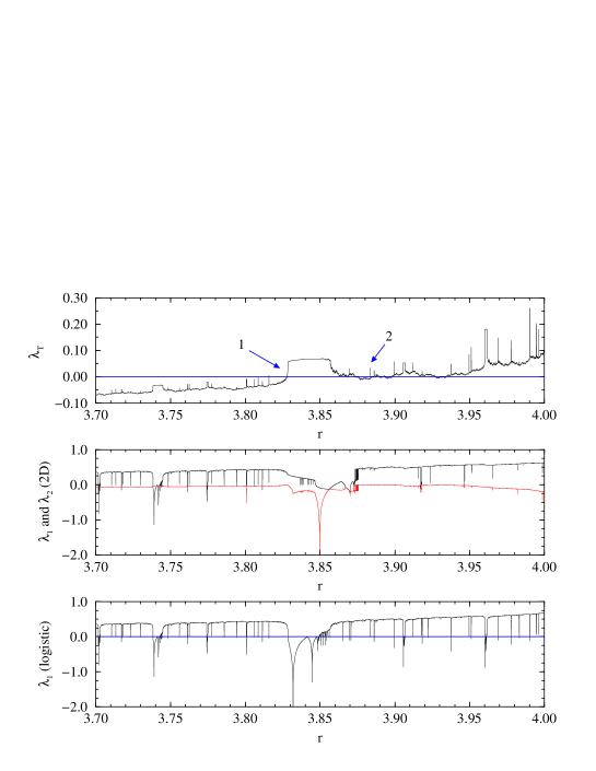
Figure 1: Numerically computed LEs of attractors for the system (1), upon changing the non-normal parameter $r$. Here $\lambda_{T}$ and $\lambda_{1}$ (logistic) are respectively the transverse and tangential exponents for an attractor in $f|_{N}$ (i.e. with initial condition $y=0$), and $\lambda_{1}$ and $\lambda_{2}$ (2D) refer to the LEs for an attractor of the full system. The regions marked by 1 and 2 in the top panel correspond to different occurrences of “blurred blowout bifurcations”, where $\lambda_{T}$ passes through $0$. The other parameters are fixed at $(s,\nu,a,b)=(-0.3,1.82,-1,-1)$

(a)

(b)

Figure 2: Panel (a) represents the phase space picture for the full system (1) for parameter values $r=3.8285$, $\nu=1.82$, $s=-0.3$, $a=-1$ and $b=-1$ (in the region marked 1), and initial conditions $x=1/2$, $y=1/2$, whereas panel (b) represents a similar picture (corresponding to region marked 2) with parameter values $r=3.88615$, $\nu=1.82$, $s=-0.3$, $a=-1$ and $b=-1$ and initial conditions $x=1/2$, $y=1/2$.

We have also calculated in each case the average distances and maximum distance of typical trajectories from $N$ and LEs after transients have been allowed to die away. These are shown in Figures 3 and 4.

The regime 1 corresponding to $r=3.828$ is brought about by a saddle-node going to a stable period $3$ orbit in $N$ that breaks down to chaos on reducing $r$ via saddle-node induced intermittency. The regime 2 located near $r=3.886$ seems to have attractors that barely vary their statistics.

In both cases the blowout is observable over a small range of $r$. As shown in Figures 3(d) and 4(d), the transverse LE appears to vary non-differentially over a large measure set of $r$. We suppose that these show essentially the same phenomenon, with just a different measure set of points where ‘blowout’ bifurcations occur.

Figure 3: Details of the LEs (a,c,d) and the average and maximum distances (b) of a typical trajectory from the invariant manifold $N$ for attractors of the map (1), in the region marked 1. The minimum distance is always very close to zero and hence has been excluded. (d) shows a seemingly non–differentiable change in transverse Lyapunov exponent as a function of $r$, organised by a saddle-node to intermittency at $r=3.828$. Note however the “spikes” in $\lambda_{T}$ in the chaotic regime, $r<3.282$, indicating the locking onto large periodic orbits that are very close in invariant measure to the period three orbit existing for $r>3.282$. Increasing the number of iterates does not seem to affect the structure of this figure. The other parameters are fixed at $(s,\nu,a,b)=(-0.3,1.82,-1,-1)$.

Figure 4: Details of the LEs (a,c,d) and the average and maximum distances (b) of a typical trajectory from the invariant manifold $N$ for attractors of the map (1), in the region marked 2, where the transients have been allowed to decay. The minimum distance is always very close to zero and hence has been excluded, implying that all attractors are “stuck on” to $N$ if they are not actually within $N$. (d) shows an apparently non–differentiable change in transverse Lyapunov exponent as a function of $r$, resulting in a blurred blowout near $r=3.8866$. Increasing the number of iterates does not seem to affect the structure of this figure. The other parameters are fixed at $(s,\nu,a,b)=(-0.3,1.82,-1,-1)$.

Figure 5: Successive scan with amplifications through the two dimensional parameter space $(\nu,r)$, showing regions of transverse stability (below the boundary curve) and transverse instability (above the boundary curve) of typical attractors in $N$. The other parameters are fixed at $(s,a,b)=(-0.3,-1,-1)$. This boundary has locally the form of a graph over $r$ because $\nu$ is a normal parameter.

Finally, Figure 5 shows the boundaries of the regions in the 2–dimensional $(r,\nu)$ parameter space for which the attractor in $N$ is transversely stable (unstable). Note how there are two regions in this parameter space; one in which there is an attractor contained in the invariant subspace and another where there is not. The boundary between the two takes the form of a graph over $r$. This is because $\nu$ is a normal parameter and so for a given attractor in $N$ this varies the normal LE smoothly through zero. The lack of normality of $r$ means that the variation is much more complicated in this direction.

These numerical computations demonstrate a number of important features of the blowout bifurcations observed here, notably:

• There are oscillations through zero of the transverse Lyapunov exponent of the attractor for the map $h$.

• The set of parameter values where the tangential LE is positive (corresponding to a chaotic attractor for $h$) are interrupted by a large number of intervals where the LE is negative and the dynamics is periodic.

• The minimum distance from $N$ is always observed to be exactly (or very close to) zero, implying that all attractors are “stuck on” to $N$ if they are not actually within $N$.

On the basis of results in the next section, we conjecture that there is in fact a positive measure set of $r$ that correspond to blowout bifurcations in some sense.

2.2.2 Intermittent behaviour

(a)

(b)

Figure 6: Panels (a) and (b) show examples of time series generated by iterating (1) from a randomly chosen initial condition, after transients have been allowed to die out. In each case, the top plot shows $y$ in a logarithmic scale, and the second and the third plots show $x$ and $y$ on linear scales. Panel (a) shows an example of on-off intermittency at $r=3.82786$ ($\lambda_{T}=0.0024$) and panel (b) an example of what we refer to as in-out intermittency at $r=3.88615$ ($\lambda_{T}=0.023$). The other parameters are fixed at $(s,\nu,a,b)=(-0.3,1.82,-1,-1)$.

Figure 6 shows two examples of intermittent-type behaviour for the system (1), involving an attractor that is not in $N$ but which contains points arbitrary close to $N$. Figure  6(a) shows an example of the well-known on-off intermittency [28]; while Figure  6(b) shows an example of a related intermittency (in-out intermittency) where the attractor in $N$ is much smaller than the attractor for the full system intersected with $N$. In the latter case, the statistics of the attractor on $N$ are markedly different from the statistics of the attractor for the full system near $N$. This is reflected by the “windows” of periodic behaviour in the $x$ dynamics when $y$ is small and growing exponentially over several orders of magnitude. Section 4 presents a theoretical analysis and characterisation of this type of intermittent behaviour.

2.2.3 Non-normal riddling bifurcation

Suppose there is a minimal attractor $A\subset N$ with a (locally) riddled basin [1, 6] that is fragile. On varying a non-normal parameter it is possible for this to collapse onto a stable periodic orbit within $N$ under arbitrarily small perturbations. If the periodic orbit is linearly stable we can infer that its basin of attraction has open interior and so upon variation of a non-normal parameter we can get transitions from open basins to and from riddled basins in a very natural way.

This transition to riddled basins will in general be “blurred” as with the blowout bifurcation. Figure 7 shows an example of basins of attraction of attractors within $N$ computed for the map (1) at two different but close values of $r$. In one case the attractor in $N$ is periodic and in the other a chaotic attractor in $N$ with a riddled basin. Between these two values there will be a non-normal riddling bifurcation (or more precisely, a set of such bifurcations). We note that despite their apparent similarity, the sets in Figs. 7(a) and 7(b) are fundamentally different. To see this we show details in Figs. 8(a) and 8(b), where the hyperbolic periodic attractor in $N$ clearly shows the presence of open sets.

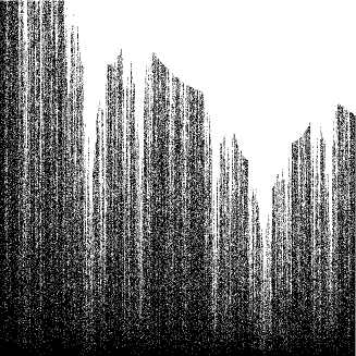
(a)

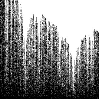
(b)

Figure 7: The white regions show the local basin of attraction of (a) a chaotic attractor in $N$ and (b) a hyperbolic periodic attractor in $N$. In case (a) the basin is riddled whereas in (b) the basin is open. Even though the two sets look very similar; they differ fundamentally on a finer scale. Points in black are attracted to $N$ without leaving $y>0.1$, while those in white cross the threshold $y>0.1$ before going to $N$. The coordinate region depicted by the figures is given by $x=[0,1]$, $y=[0,0.1]$, and the parameters are fixed at $(r,s,\nu,a,b)=(3.886,-0.3,0.545,-1,1)$ and $(r,s,\nu,a,b)=(3.88605,-0.3,0.545,-1,1)$ in (a) and (b) respectively.

(a)

(b)

Figure 8: Detail of Figure 7(a) and (b). Panel (b) clearly shows the presence of open sets (the existence of the open set can also be inferred by noting that there is a linearly stable periodic point at the centre of the bottom of this figure). The coordinate regions depicted here is given by $x=[0.49,0.51]$, $y=[0,0.05]$.

3 Non-normal parameters: theory

We explain the new observed effects of non-normal blowout, in-out intermittency and non-normal riddling in the context of a recent conjecture of Barreto et al.  [9] on the parameter dependence of chaotic attractors.

3.1 Fragile chaos and the windows conjecture

Barreto et al.  consider a class of chaotic attractors that are fragile, i.e. attractors that are not structurally stable under perturbations, but that nonetheless persist for a large measure of nearby parameter values. Such attractors are thought to be present in a large number of physically important systems. More precisely, Barreto et al.  suppose that a mapping $h$ has a chaotic attractor $A$ possessing $k\geq 0$ positive LEs. Suppose that $h^{\prime}$ is a mapping that is $C^{1}$ close to $h$ and such that almost all points in a neighbourhood of $A$ are attracted to periodic orbits. Then they say $A$ is dispelled for $h^{\prime}$. They define the attractor $A$ as being fragile if $A$ is dispelled for $C^{1}$-arbitrarily close $h^{\prime}$.

In particular, their main conjecture (the windows conjecture) for one parameter and one positive LE, suggests that there will be a dense set of nearby parameter values at which the attractors are periodic. This set of parameter values is called the windows set.

For the model (1) that we consider, there are two deep results about the logistic map that mean that the chaotic attractors of the map on $N$ are really fragile in the above sense. Namely:

Theorem 1

(see [18, 13]) Consider the mapping $f_{a}(x)=ax(1-x)$ from $[0,1]$ to itself. There is a positive measure subset $I_{c}$ of $[0,1]$ such that $a\in I_{c}$ implies that $f_{a}$ has a chaotic attractor with absolutely continuous invariant measure and one positive LE. The complement of this set contains an open and dense subset $I_{p}\subset[0,1]$ such that $a\in I_{p}$ implies that almost all points are attracted to a stable periodic orbit.

3.2 Attractors and invariant measures

We briefly sketch some standard definitions and results that we need. Suppose $f:{\bf R}^{m}\rightarrow{\bf R}^{m}$. If $A\subset{\bf R}^{m}$ is a compact invariant set then we define

$${\cal W}^{s}(A)=\{x\in{\bf R}^{m}~{}:~{}\omega(x)\subseteq A\}$$

to be the stable set or basin of attraction of $A$; similarly we define

$${\cal W}^{u}(A)=\{x\in{\bf R}^{m}~{}:~{}\alpha(x)\subseteq A\}$$

to be the unstable set of $A$.

Suppose that $\ell$ is Lebesgue measure on ${\bf R}^{m}$. Following Milnor [22], we say $A$ is an attractor if $\ell({\cal W})>0$. It is a minimal attractor if there is no compact invariant proper subset $A^{\prime}\subset A$ with $\ell({\cal W}^{s}(A^{\prime}))=\ell({\cal W}^{s}(A))$.

Suppose that $A$ is an attractor in the sense of Milnor. We say it possesses a natural measure if there is an ergodic invariant measure $\mu$ supported on $A$ such that almost all points in ${\cal W}^{s}(A)$ are generic for $\mu$; i.e. if almost all $x\in{\cal W}^{s}(A)$ satisfy

$$\lim_{n\rightarrow\infty}\frac{1}{n}\sum_{k=0}^{n-1}\phi(f^{k}(x))=\int\phi\,d\mu.$$

for all compactly supported $\phi\in C^{0}({\bf R}^{m},{\bf R})$.

Note that if $A$ supports chaotic dynamics then typically there are many other ergodic invariant measures supported on $A$; these are the singular measures:

$${\cal M}_{A}=\{\nu~{}\mbox{ ergodic invariant measures }~{}:~{}\mbox{supp}(\nu)\subseteq A\}$$

and include, for example, measures supported on unstable periodic motions contained within $A$.

The basic result of Oseledec’s theorem [23] is that LEs exist and take a finite number of constant values on a set of full $\nu$-measure for any ergodic $\nu$. If $A$ has a natural measure as well as singular measures we say the attractor is chaotic and the LEs to almost all initial points are given by those for the natural measure; however the convergence is non-uniform and shows arbitrarily long deviations towards the LEs for any singular measure for $A$. This causes riddling and several other phenomena associated with chaotic behaviour in an invariant subspace.

As shown, for example, in [31, 27, 1, 7], for a large class of attractors one can classify an attractor in an invariant subspace according to its transverse LEs according to where zero lies relative to this spectrum. Suppose that $\mu_{\nu}$ is a family of natural measures of attractors for $h_{\nu}$ and define

$$\lambda_{T}(\nu)=\max\{\lambda_{\perp}(\mu_{\nu}))\}$$

the most positive transverse LE for the natural measure at $\nu$. Then $A_{\nu}=\mbox{supp}(\mu_{\nu})$ is an attractor for $f_{\nu}$ if $\lambda_{\nu}<0$. It is not an attractor if $\lambda_{T}(\nu)>0$. Parameter values $\nu_{0}$ where $\lambda_{T}$ takes both signs for $\nu$ arbitrarily close to $\nu_{0}$ we refer to as blowout points of $A_{\nu}$ and these govern the bifurcation from the invariant subspace [26].

3.3 Blowout with normal parameters

The transverse LEs can be thought of as the characteristic exponents for the linear skew product system

$$\tilde{f}_{\nu}(x,v)=(h(x),M_{\nu}(x)v)$$

where $M(x)$ is a normal derivative at $x$; i.e. such that

$$D_{(x,0)}f_{\nu}\left(\begin{array}[]{c}{u}\\ {v}\end{array}\right)=\left(\begin{array}[]{cc}{*}&{*}\\ {0}&{M_{\nu}(x)}\end{array}\right)\left(\begin{array}[]{c}{u}\\ {v}\end{array}\right),$$

where $*$ denotes some matrix function of $x$. If we consider such a system perturbed by normal parameters, the transverse LEs are simply those of a perturbed cocycle and so in particular they can vary continuously with any normal parameter (more precisely, they will vary continuously on a generic set of perturbed systems [2]). If the LEs do vary continuously then in particular $\lambda_{T}$ will vary continuously and even

$$\frac{d\lambda_{T}}{d\nu}\neq 0$$

generically for $\lambda_{T}=0$; thus we can see that (at least within an open set of smooth systems), generically the set of blowout points has codimension one in parameter space. On one side of such a normal blowout, $A_{\nu}$ is an attractor for $f_{\nu}$; on the other side it is not. When $A_{\nu}$ loses stability it may give rise to a branch of on-off intermittent attractors (non-hysteretic or supercritical scenario), or there may be no nearby attractors (hysteretic or subcritical scenario), as discussed by Ott & Sommerer (although there are further possibilities, as discussed in [8]). Note that the hysteretic scenario may give rise to transient on-off intermittent behaviour [34] near blowout.

3.4 Blowout with non-normal parameters and the blowout set

If we do not have normal parameters and have fragile chaos in the invariant subspace, the attractors $A_{\nu}$ will typically collapse over some dense set of windows and consequently $\lambda_{\nu}$ will typically not vary continuously.

As $\lambda_{T}(\nu)$ does not vary continuously we cannot apply any intermediate value theorem and so it is possible to pass from $\lambda_{T}<0$ to $\lambda_{T}>0$ without passing through zero. Therefore, we define

$$I^{+}=\{\nu~{}:~{}\lambda_{T}(\nu)\geq 0\},~{}~{}I^{-}=\{\nu~{}:~{}\lambda_{T}(\nu)\leq 0\}$$

and the blowout set to be

$$I^{0}=\partial I^{+}\cap\partial I^{-}=\overline{I^{+}}\cap\overline{I^{-}}.$$

For normal parameters, this is equivalent to the set of blowout bifurcations. The numerical evidence of Section 2 suggests that $I^{0}$ can be a fractal: more precisely we can use Theorem 1 to show the following.

Corollary 1

There is a map of the form (1) whose blowout set $I^{0}$ has positive Lebesgue measure in parameter space.

Proof: Consider any map that has linear form

$$f_{a}(x,y)=(ax(1-x),(a-2ax)y)$$

near the invariant subspace $y=0$. This is such that the tangential and the transverse LEs are the same for all $a$. On varying the non-normal $a$, it is possible to see that $I^{+}=I_{c}$ and $I^{-}=I_{p}$ in the notation of Theorem 1; the conclusions of this theorem imply that $I^{0}=I^{+}$ and consequently the blowout set has positive Lebesgue measure.

QED

In the more general case of $A$ being an attractor that is stuck on to $N$ with $A_{0}=A\cap N$ fragile then we conjecture that there are typically positive measure blowout sets at loss of transverse stability. If $A_{0}$ is not fragile but instead structurally stable (e.g. if it is uniformly hyperbolic) then the blowout set has zero Lebesgue measure. However, even in the case of a positive measure blowout set, the sparcity of windows may mean that they are very difficult to observe even in a region where they exist.

4 In-out intermittency

We now turn to a static (i.e. non-bifurcation) effect that is associated with the blurred blowout. In particular, we characterise a generalised form of on-off intermittency that we refer to as in-out intermittency. This includes forms of on-off intermittency where the attracting dynamics within the invariant subspace does not need to be chaotic.

In the following, we will suppose we have a minimal Milnor attractor $A$ for $f$ such that $A_{0}=A\cap N$ is non-empty and $A\cap N^{c}$ is also non-empty.

We write ${\cal A}$ to be the set of invariant subsets of $A_{0}$ and define

$${\cal A}_{0}^{*}=\{B\subset A_{0}~{}:~{}B\mbox{ is a minimal attractor for $f|_{N}$}\}$$

and

$$A_{0}^{*}=\overline{\cup_{B\in{\cal A}^{*}}B}.$$

This is a closed invariant subset of the invariant set $A_{0}$. We can think of $A_{0}^{*}$ as the set of points that attract almost all points within $A^{0}$. If

$$A_{0}^{*}=A_{0}$$ (3)

then we say the attractor $A$ displays on-off intermittency. In the more general case where

$$A_{0}^{*}\subseteq A_{0}$$ (4)

we say that $A$ displays in-out intermittency, implying that the attraction and repulsion to the invariant subspace are dominated by different dynamics.

Hypothesis We will assume that if $f$ has a Milnor attractor $A$ and $A_{0}=A\cap N$ is non-empty for some invariant manifold $N$ then $A_{0}$ is a Milnor attractor for $f|_{N}$.

Note that if $A$ is an asymptotically stable attractor then this will always hold; at present we have no measurable examples where this fails to hold but are not aware of a sufficiently general setting where this will always hold. Therefore we will leave it as a standing hypothesis. Necessarily this means that $A_{0}^{*}$ will be non-empty, but it may be a proper subset of $A_{0}$.

4.1 Skew product systems

The original examples of on-off intermittency and much theory has been developed for skew product systems. Interestingly enough, non-trivial in-out intermittency cannot occur in such a system, as the following result implies.

Lemma 1

Suppose that $f$ has skew product form (2) and $A$ is a minimal Milnor attractor for $f$. Then $A_{0}=A\cap N$ is a minimal attractor for $g=f|_{N}$.

Proof: Suppose $\Pi:{\bf R}^{m}\rightarrow N$ defined by $\Pi(x,y)=x$ is the orthogonal projection onto $N$. If $f$ has form (2) then $\Pi\circ f=g\circ\Pi$ shows that $g$ is a factor of $f$. This means that $A_{0}$ is compact and invariant and moreover, ${\cal W}^{s}(A_{0})\cap N=\Pi({\cal W}^{s}(A))$; since the image of a set with positive $m$ dimensional Lebesgue measure under $\Pi$ has positive $n$ dimensional measure, this means that $A_{0}$ is a Milnor attractor for $g$. Suppose that $A_{0}$ is not minimal for $g$. Then there will be a positive measure subset of ${\cal W}^{s}(A_{0})\cap N$ that converge to some proper compact subset $B\subset A_{0}$. Thus there will be a positive measure subset of ${\cal W}^{s}(A)$ that converge to a set $B^{\prime}$ with $\Pi(B^{\prime})=B$ and $B^{\prime}\subset A$. Taking the closure of $B^{\prime}$, this contradicts the assumption that $A$ is minimal.

QED

The following theorem is a direct result of Lemma 1.

Theorem 2

If $A$ is a minimal Milnor attractor for a skew product system and $A$ displays in-out intermittency then it displays on-off intermittency.

If $f$ is not a skew product then $A_{0}^{*}$ can be a proper subset of $A_{0}$. For example, see the illustration in Figure 9 of a heteroclinic network in ${\bf R}^{2}$ where the only minimal attractor in $N$ is a fixed point.

Figure 9: Heteroclinic cycle consisting of two equilibria in $N$ connections between them. If this forms part of an attractor then the only minimal attractor within $N$ is the fixed point that is stable within $N$.

The existence of in-out intermittency forces several consequences in terms of LEs (where $\lambda_{T}(\mu)=\max\lambda_{\perp}(\mu)$ for an invariant measure $\mu$):

Lemma 2

Suppose that $A$ is an attractor displaying in-out intermittency and $A_{0}^{*}$ has a natural measure $\mu^{*}$ for $f|_{N}$. Then (i) $A_{0}$ is not uniquely ergodic, (ii) $\lambda_{T}(\mu^{*})\geq 0$ and (iii) there exists a measure $\mu^{\dagger}$ with support on $A_{0}\setminus A_{0}^{*}$ such that $\lambda_{T}(\mu^{\dagger})\leq 0$.

Proof: (i) Is a trivial consequence of the fact that $A_{0}^{*}\neq A_{0}$. (ii) Suppose that $\lambda_{T}(\mu^{*})<0$; then $A_{0}^{*}$ is a minimal attractor for $f$. (iii) Likewise, if this were not the case then $A^{0}$ would be an attractor for $f$.

QED

As far as the dynamics on $A_{0}$ and the minimal attractors $A_{0}^{*}$ go there seem to be many possibilities. In the numerical example, we see examples where $A_{0}$ is a chaotic repellor and $A_{0}^{*}$ is periodic. There is no reason why $A_{0}^{*}$ should be composed of a single minimal attractor, or indeed why $A_{0}^{*}$ itself should not be chaotic.

We now address the question of how to model the in-out intermittent states themselves; we do this with the aid of a Markov model.

4.2 A Markov model of in-out intermittency

We motivate, describe and analyse a Markov chain model of in-out intermittency that enables us to predict scalings associated with this form of intermittency. In particular we consider the laminar phases, corresponding to phases where the trajectory is below a given threshold from the invariant submanifold. Note that unlike the case for on-off intermittency, we do not have a corresponding Fokker-Planck equation which models this Markov model (cf [27]).

Consider a Markov chain described by two semi-infinite chains of states $P_{i}$ and $Q_{i}$, $i=0,1,2,\ldots$. We call the chain $P_{i}$ the “in” chain and $Q_{i}$ the “out” chain. We assign transition probabilities as shown in Table 1 and show the chain schematically in Figure 10. This model has three parameters

$$\alpha_{U},~{}~{}\alpha_{D}~{}~{}\mbox{ and }~{}~{}\epsilon$$

which are all positive and such that $\alpha_{U}+\alpha_{D}+\epsilon\leq 1$. For simplicity we assume that $\alpha_{U}+\alpha_{D}+\epsilon=1$ and so the transition from $P_{i}$ to $P_{i}$ cannot happen. In this case we can reparametrise using $\lambda\in{\bf R}$ by defining

$$\alpha_{U}=\frac{1-\epsilon+\lambda}{2},~{}~{}\alpha_{D}=\frac{1-\epsilon-\lambda}{2}.$$

and note that $\lambda$ corresponds to a bias in the drift on the “in” chain.

$$\begin{array}[]{c|cccccc}&\lx@intercol\hfil\mbox{To}\hfil\lx@intercol\\ &P_{i-1}&P_{i}&P_{i+1}&Q_{i-1}&Q_{i}&Q_{i+1}\\ \hline\cr P_{i}&\alpha_{U}&1-\alpha_{U}-\alpha_{D}-\epsilon&\alpha_{D}&0&\epsilon&0\\ Q_{i}&0&0&0&1&0&0\\ \end{array}$$

($i\geq 2$)

$$\begin{array}[]{c|ccc}&\lx@intercol\hfil\mbox{To}\hfil\lx@intercol\\ &P_{1}&P_{2}&Q_{1}\\ \hline\cr P_{1}&1-\alpha_{D}-\epsilon&\alpha_{D}&\epsilon\\ Q_{1}&1&0&0\\ \end{array}$$

Table 1: Probability of transition from the states $P_{i}$ and $Q_{i}$ for $i\geq 1$ in the Markov model of in-out intermittency. The $P_{i}$ model a biased random walk that can leak onto a deterministic motion away from $\infty$. At $i=1$ the $Q_{i}$ chain feeds into the $P_{i}$ chain.

Figure 10: Schematic diagram showing transitions in the Markov model for in-out intermittency. The site $i$ can be thought of as indexing a distance $\gamma^{i}$ from the invariant manifold for some $\gamma<1$ and so we approach the invariant subspace on letting the index $i\rightarrow\infty$.

Equilibrium distributions

We compute equilibrium probability distributions $p_{i}$ and $q_{i}$ of the above model by solving the linear recurrence relations:

$$p_{i} = \alpha_{U}p_{i+1}+\alpha_{D}p_{i-1}+(1-\alpha_{U}-\alpha_{D}-\epsilon)p_{i},~{}~{}i\geq 2$$

$$q_{i} = q_{i+1}+\epsilon p_{i},~{}~{}i\geq 2$$

$$p_{1} = \alpha_{U}p_{2}+q_{1}+(1-\epsilon-\alpha_{D})p_{1}.$$

Expressing in terms of the parameters $\lambda$ and $\epsilon$ we use an ansatz $p_{i}=\mu^{i}$ to obtain

$$q_{i} = \frac{\epsilon}{1-\mu}\mu^{i}$$ (5)

$$p_{i} = \mu^{i}$$ (6)

where $\mu$ satisfies

$$(1-\epsilon+\lambda)\mu^{2}-2\mu+(1-\epsilon-\lambda)=0.$$

This quadratic equation has solutions

$$\frac{1\pm\sqrt{\lambda^{2}+2\epsilon-\epsilon^{2}}}{1-\epsilon+\lambda}$$

but we are only interested in normalised probability measures; this means that the only physically relevant solution (with $|\mu|\leq 1$) is

$$\mu=\frac{1-\sqrt{\lambda^{2}+2\epsilon-\epsilon^{2}}}{1-\epsilon+\lambda}.$$

For normalisation, the sum over all probabilities is unity

$$1=\sum_{i=1}^{\infty}C(p_{i}+q_{i})=C\frac{\epsilon+1-\mu}{(1-\mu)^{2}},$$ (7)

giving $C=\frac{(1-\mu)^{2}}{\epsilon+1-\mu}$. Now the asymptotic ratio between time spent in the “in” and “out” phases, $R_{io}$, which is a dynamical invariant, can be easily calculated as

$$R_{io}=\frac{\sum_{i=1}^{\infty}Cp_{i}}{\sum_{i=1}^{\infty}Cq_{i}}=\frac{1-\mu}{\epsilon}$$ (8)

and the average value of the transverse variable $y$ can be similarly found to be

$$<y>=\sum_{i=1}^{\infty}C(p_{i}+q_{i})\gamma^{-i}=\frac{(1-\mu)\gamma}{\gamma-\mu}.$$ (9)

This quantity $R_{io}$ can be seen to be an invariant of the system up to conjugacy and so is a quantity by which the intermittency can be characterised. The case $R_{io}=\infty$ (equivalently $\epsilon=0$) corresponds to when the trajectory stays on the “in” phase and hence performs on-off intermittency. In the case $R_{io}\ll 1$, the trajectory will spend long times moving away from the invariant subspace on the “out” phase interspersed with short and necessarily fast-moving contractions towards the invariant subspace. We have seen examples of in-out intermittency in the map (1) that show a wide range of $0\leq R_{io}<\infty$.

Note that $\log\gamma$ corresponds to the transverse LE $\lambda_{T}$ for the “out” phases. Usually for systems with normal parameters, the average laminar phase as a function of $(r-r_{c})$, where $r_{c}$ is the value of $r$ for which the blowout bifurcation occurs, scales as $<y>^{-1}$. If there is a scaling between $<y>$ or $R_{io}$ and the normal parameters $\nu$, $a$, $b$ or $s$, then we can go further and obtain $\mu$.

Therefore, we can use this model for any in-out intermittent attractor by identifying

$$\lambda_{T},~{}~{}\lambda,~{}\mbox{ and }~{}\epsilon,$$

or equivalently, by measuring

$$\lambda_{T},~{}~{}R_{io},~{}~{}\mu~{}\mbox{ and }~{}<y>$$

and computing $\gamma$, $\lambda$, $\mu$ and $\epsilon$ via

$$\mu = \frac{1-\sqrt{\lambda^{2}+2\epsilon-\epsilon^{2}}}{1-\epsilon+\lambda}$$

$$R_{io} = \frac{\epsilon}{1-\mu}$$

$$<y> = \frac{(1-\mu)\gamma}{\gamma-\mu}$$

$$\lambda_{T} = \log\gamma.$$

We can also calculate the average length of “out” phases, $L_{o}$ as

$$L_{o}=\sum_{i=1}^{\infty}Cq_{i}=\frac{1}{1-\mu-\epsilon}.$$ (10)

Note that it would be equally possible to have more than two chains corresponding to, for example, more than one type of “out” dynamics. Equally, the out dynamics could be chaotic and give rise to a biased but two-directional random walk on the out-chain. There are many possibilities and we do not examine all of these in detail on this occasion, however we have observed such behaviours in the model mapping (1).

4.3 Scalings of laminar phases

We now compute long time asymptotic properties of the scaling of laminar phases for in-out intermittency by analysing the Markov model proposed in the previous section. We find that for small $\epsilon$ this is very similar to that found for on-off intermittency; namely for small times it decays according to a power law $n^{-3/2}$ whereas for larger times it decays much faster, namely exponentially.

To compute the distribution we consider a trajectory starting at some site on the “in” chain and consider the distribution of times as to when it returns for the first time to that site in the “in” chain. Suppose we want to find the probability of the trajectory returning for the first time after $2n$ steps. This can occur either by the trajectory remaining in the “in” chain for that excursion, or it can happen by ‘leaking’ onto the $2n-2l$th site further down the “out” chain after a time $2l$ and then propagating up the “out” chain for the remaining time.

More precisely, let

$$S_{2n}=P\{\mbox{first return is after time $2n+2$}\}$$

where this is computed assuming that we start at a given site on the “in” chain and $P_{in}(2n+2)$ the probability of the first return occur at time $2n+2$ always in the “in” chain. Let

$$T_{2n}(2l)=P\{\mbox{attains site $2l$ after a time $2n$, has not returned or switched before then}\}.$$

Then we can compute

$$S_{2n}=P_{in}(T=2n+2)+\epsilon\sum_{l=\lceil n/2\rceil}^{n-1}T_{2l}(2n-2l).$$

Using a directed version of the probability of the first return and the hitting time formulas [15, 14] given by

$$P_{in}(T=2n+2)=\frac{1}{n+1}\left(\begin{array}[]{c}{2n}\\ {n}\end{array}\right)(\alpha_{D}\alpha_{U})^{n+1}$$

and

$$T_{2n}(2l)=\frac{l}{n}\left(\begin{array}[]{c}{2n}\\ {n+l}\end{array}\right)(\alpha_{D})^{n+l}(\alpha_{U})^{n-l}$$

respectively, we obtain, for $\alpha_{U}\neq 0$,

$$S_{2n} = \frac{1}{n+1}\left(\begin{array}[]{c}{2n}\\ {n}\end{array}\right)(\alpha_{D}\alpha_{U})^{n+1}+\epsilon\sum_{l=\lceil n/2\rceil}^{n-1}\frac{n-l}{l}\left(\begin{array}[]{c}{2l}\\ {n}\end{array}\right)(\alpha_{D})^{n}(\alpha_{U})^{2l-n}$$

$$= \frac{1}{n+1}\left(\begin{array}[]{c}{2n}\\ {n}\end{array}\right)(\alpha_{D}\alpha_{U})^{n+1}+\epsilon\left(\frac{\alpha_{D}}{\alpha_{U}}\right)^{n}\sum_{l=\lceil n/2\rceil}^{n-1}\frac{n-l}{l}\left(\begin{array}[]{c}{2l}\\ {n}\end{array}\right)(\alpha_{U})^{2l}.$$

It now remains to find the asymptotic behaviour of this expression. Using Stirling’s formula $n!\sim n^{n+\frac{1}{2}}e^{-n}\sqrt{2\pi}$ we have

$$\left(\begin{array}[]{c}{2n}\\ {n}\end{array}\right)\sim\frac{4^{n}}{\sqrt{n\pi}}$$

which upon taking $n\rightarrow\infty$ gives

$$S_{2n} \sim \alpha_{U}\alpha_{D}\,n^{-\frac{3}{2}}\frac{(4\alpha_{U}\alpha_{D})^{n}}{\sqrt{\pi}}$$

$$+\epsilon\left(\frac{\alpha_{D}}{\alpha_{U}}\right)^{n}\frac{1}{n^{n}\sqrt{2\pi n}}\sum_{l=\lceil n/2\rceil}^{n-1}\frac{n-l}{l}(2l)^{2l+\frac{1}{2}}(2l-n)^{-2l+n-\frac{1}{2}}(\alpha_{U})^{2l}$$

$$= I_{1}+I_{2}.$$

We can approximate $I_{2}$ by

$$I_{2} \sim \epsilon\left(\frac{\alpha_{D}}{\alpha_{U}}\right)^{n}\frac{1}{n^{n}\sqrt{2\pi n}}\int_{x=\lceil n/2\rceil}^{n}\frac{n-x}{x}(2x)^{2x+\frac{1}{2}}(2x-n)^{-2x+n-\frac{1}{2}}(\alpha_{U})^{2x}\,dx$$

which by changing the integration variable to $x=n(1+y)/2$ becomes

$$I_{2} \sim \epsilon\left(\frac{\alpha_{D}}{\alpha_{U}}\right)^{n}\frac{\sqrt{n}}{\sqrt{2\pi}}\int_{0}^{1}\frac{1-y}{\sqrt{(1+y)y}}(1+y)^{n(1+y)}y^{-ny}(\alpha_{U}^{n})^{1+y}\,dy$$

$$\sim \epsilon\left(\frac{\alpha_{D}}{\alpha_{U}}\right)^{n}\frac{\sqrt{n}}{\sqrt{2\pi}}\int_{0}^{1}q(y)e^{np(y)}\,dy$$

where $p(y)=(1+y)\log((1+y)\alpha_{U})-y\log y$ and $q(y)=\frac{1-y}{\sqrt{y(1+y)}}$. Note that $p(y)$ has a single maximum at $y_{m}\in[0,1]$ given by solving

$$p^{\prime}=\log(\alpha_{U}(1+y))-\log y=0$$

and $p^{\prime\prime}(y)=\frac{1}{1+y}-\frac{1}{y}$. We need at this point to distinguish between two cases for $\alpha_{U}$.

Case of $0<\alpha_{U}<\frac{1}{2}$

In this case, $y_{m}=\frac{\alpha_{U}}{1-\alpha_{U}}$ and the maximum $y_{m}$ is in the interior of the range of integration. Laplaces’ method gives

$$\int_{0}^{1}q(y)e^{np(y)}\,dy\sim q(y_{m})e^{np(y_{m})}\frac{1}{\sqrt{-2\pi np^{\prime\prime}(y_{m})}}$$

asymptotically as $n\rightarrow\infty$ and so we can estimate

$$I_{2}\sim\frac{\epsilon}{2\pi}\frac{2\alpha_{U}-1}{\alpha_{U}-1}\left(\frac{\alpha_{D}}{1-\alpha_{U}}\right)^{n}$$

to leading order. Note that this implies that $I_{1}\ll I_{2}$ and $I_{2}$ gives exponential fall off of $S_{2n}$ in $n$ for large $n$. Note however the factor $\epsilon$ in $I_{2}$ means that $I_{1}$ may dominate the statistics up to a moderately large values of $n$.

Case of $1>\alpha_{U}>\frac{1}{2}$

In this case $y_{m}=1$ and $p^{\prime}(1)>0$. This means that the leading term in $I_{2}$ is given by

$$I_{2}\sim\epsilon n^{-\frac{3}{2}}(4\alpha_{D}\alpha_{U})^{n}$$

as $n\rightarrow\infty$. This is the same scaling with $n$ as for $I_{1}$ and so it will appear to scale exactly as for on-off intermittency. Thus in this case

$$S_{2n}\sim n^{-\frac{3}{2}}(4\alpha_{U}\alpha_{D})^{n}$$

in the limit of large $n$. Rewriting this as

$$S_{2n}\sim n^{-\frac{3}{2}}\exp(n\log(4\alpha_{U}\alpha_{D}))$$

we note that for any $\epsilon>0$

$$0<4\alpha_{U}\alpha_{D}=(1-\epsilon)^{2}-\lambda^{2}<1$$

and so $S_{2n}$ scales as $n^{-3/2}$ up to the point where exponential decay sets in.

Other cases

In the case $\alpha_{U}=\frac{1}{2}$ we note that $y_{m}=1$ and $p^{\prime}(1)=0$; we do not consider this case in detail. In the case $\alpha_{U}=0$ we have a deterministic propagation down the “in” chain and it is easy to compute that

$$S_{2n}\sim\epsilon(1-\epsilon)^{n}$$

i.e. we have exponential decay only, and no $n^{-\frac{3}{2}}$ scaling. This case is the limiting case where $\lambda\rightarrow\epsilon-1$.

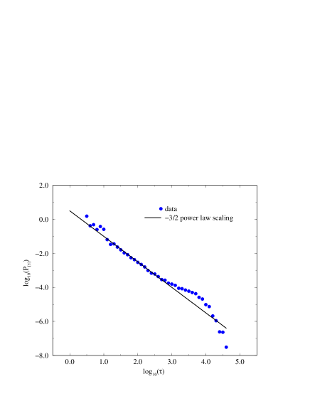
Figure 11: Scaling law for proportion $P$ of laminar phases of length $\tau$ for in-out intermittency at $r=3.8800045$ and $\nu=1.82$, $a=-1$, $s=-0.3$ and $b=-1$. This case corresponds to a case for which $\alpha_{U}<\frac{1}{2}$. Note the $n^{-3/2}$ fall off changing to exponential for larger times.

4.4 Distribution of laminar phases: summary

We note that if $\epsilon>0$ for any value of $\lambda$ the distribution $S_{2n}$ of laminar phases of length $2n$ always decays exponentially with $n$. For large $n$, we consider two cases in detail. In the case where $\alpha_{U}>\frac{1}{2}$ we have

$$S_{2n}\sim n^{-3/2}e^{n\log(4\alpha_{U}\alpha_{D})}$$

($\log(4\alpha_{U}\alpha_{D})=\log((1-\epsilon)^{2}-\lambda^{2})\leq 0$ with equality if and only if $\lambda=\epsilon=0$).

In the case of $\alpha_{U}<\frac{1}{2}$, or equivalently when $\epsilon>\lambda$, there is an asymptotic scaling of the form

$$S_{2n}\sim\frac{\alpha_{U}\alpha_{D}}{\sqrt{\pi}}n^{-3/2}e^{n\log(4\alpha_{U}\alpha_{D})}+\frac{\epsilon}{2\pi}\frac{2\alpha_{U}-1}{\alpha_{U}-1}\ e^{n\zeta}$$

where $\log(4\alpha_{U}\alpha_{D})<\zeta<0$. This causes the exponential tail to continue to much higher $n$, and indicates the presence of a higher proportion of very long laminar phases. The shoulder at high $n$ in Fig. 11 is caused by the contribution of $I_{2}$ and is a clear indicator of in-out intermittency. Pure on-off intermittency, in the noise-free case, has a scaling law which is always convex in the log-log plot. It is also possible to use these results to understand how the scaling of laminar phases varies on changing LEs in the intermittency.

5 Other bifurcations on varying a non-normal parameter

The bifurcation to riddling (and associated bifurcation to bubbling) has been discussed in detail by [24, 25, 21, 32, 33], in the case where a normal parameter is varied.

In this section we can see how basin riddling can appear on varying a non-normal parameter; this occurs via a breakdown of fragile chaos of an attractor within the invariant subspace.

5.1 Bifurcation to riddling

If we vary a non-normal parameter we expect riddled basins to typically appear and disappear in the following way;

Suppose there is a $\nu_{0}$ such that

• There is a branch of attracting periodic orbits (or more generally, uniquely ergodic attractors $B_{\nu}\subset N$ for $\nu>\nu_{0}$).

• There is a large measure subset of $\nu<\nu_{0}$ where there exist a branch of attractors $C_{\nu}\subset N$ such that $B_{\nu}$ are in a neighbourhood of the $C_{\nu}$ and the basins of the $C_{\nu}$ are locally riddled.

Then we say there is a non-normal bifurcation to riddling at $\nu_{0}$. Note that (b) holds if there is a transversely unstable measure supported on $C_{\nu}$, subject to certain regularity conditions. Some of these transversely unstable measures will continue through the bifurcation to give rise to complicated repelling sets for $\nu>\nu_{0}$.

We expect this new bifurcation is in fact a more typical way to create riddled basins on varying a non-normal parameter than the normal parameter scenario discussed in [25]. An example of the basins of attraction before and after such a bifurcation is shown in Figure 7.

5.2 Other transitions.

There are many other bifurcations that have been studied in the case of normal parameters and which will carry across to non-normal parameter systems, modulo the fact that if the chaotic invariant set in $N$ is fragile then these transitions will happen on sets that may be considerably large than codimension one.

For example, the transition to bubbling [32, 33], an attractor becoming unstuck [3] and a transition to cycling chaos [8] may all appear in a non-normal setting.

Moreover, the case $\epsilon\rightarrow 0$ in the Markov model for in-out intermittency will correspond to a transition from on-off to in-out intermittency.

6 Discussion

The motivation for this paper came from previous work of the authors [12] that investigated a truncated PDE model of an axisymmetric mean field dynamo model. Bifurcation and dynamical effects came to light that did not fit into the usual setting of a blowout bifurcation; this led us to consider these effects in the simple mapping (1).

In this paper we have addressed two main questions; firstly, what happens to a blowout bifurcation in non-skew product systems on varying the dynamics by a non–normal parameter within the invariant subspace and secondly, how to characterise the dynamics of what we call “in-out” intermittency which we suggest should be a commonly observable type of dynamics in realistic models with invariant subspaces. We have also raised a number of other questions relating to riddling and other bifurcations and discussed these in passing.

We have tried to give a general characterisation of in-out intermittency, have contrasted it to on–off intermittency and have related its likelihood to the non–skew product nature of the system and the non–normal nature of its parameters. We have proposed that this type of behaviour can be well modelled by a simple Markov chain and have used this to obtain quantitative measures of this state (notably the ratio $R_{io}$ of “in”- to “out”- states, which is a dynamical invariant).

An important signature of in–out intermittency is the presence of intervals with exponential growth in the “out” variables with a constant rate, over many orders of magnitude. While this occurs, the “in” variables closely shadow the periodic attractor in the invariant submanifold, thus giving a clear distinction from on–off intermittency where the on and off phases are not so clearly differentiated.

We shall show in a future publication that in–out intermittency can account for the behaviour observed in the study of mean field dynamo models (modelled on partial differential equations) and referred to as “icicle” intermittency by Brooke [10], who uses a skew product model to investigate this (see also Tworkowski et al.  [30] and Brooke et al.  [11]) as well as in the truncated versions of related models by the authors [12]. Similarly this type of behaviour is related to the “new type of intermittency” reported by Hasegawa et al.  [16] in a ring of phase-locked loops.

There are still few rigorous results on what has been called “fragile chaos” [9]. Further progress in the rigorous classification of non-normal blowouts is clearly hampered by the lack of these results in what is a very difficult area of analysis.

References

References

- [1] Alexander, J., Kan, I., Yorke, J. and You., Z., Riddled Basins. Int. Journal of Bifurcations and Chaos 2:795–813 (1992).
- [2] Arnold, L. and Cong, N. D., Generic properties of Lyapunov exponents. Random and Computational Dynamics 2:335–345 (1994).
- [3] Ashwin, P., Attractors stuck on to invariant subspaces. Phys. Lett. A 209:338–344 (1995).
- [4] Ashwin, P., Cycles homoclinic to chaotic sets; robustness and resonance. Chaos 7:207–220 (1997).
- [5] Ashwin, P., Aston, P. and Nicol, M., On the unfolding of a blowout bifurcation. Physica D 111:81–95 (1997).
- [6] Ashwin, P., Buescu, J. and Stewart, I., Bubbling of attractors and synchronisation of oscillators. Phys. Lett. A 193:126–139 (1994).
- [7] Ashwin, P., Buescu, J. and Stewart, I., From attractor to chaotic saddle: a tale of transverse instability. Nonlinearity 9:703–737 (1996).
- [8] Ashwin, P. and Rucklidge, A. M., Cycling chaos: its creation, persistence and loss of stability in a model of nonlinear magnetoconvection. Technical Report 97/26, Dept. of Maths and Stats, University of Surrey (1997).
- [9] Barreto, E., Hunt, B., Grebogi, C. and Yorke, J., From high dimensional chaos to stable periodic orbits: the structure of parameter space. Phys. Rev. Lett. 78:4561–4 (1997).
- [10] Brooke, J. M., Breaking of equatorial symmetry in a rotating system: a spiralling intermittency mechanism., Europhysics Letters 37:171–176 (1997).
- [11] Brooke, J.M., Pelt, J., Tavakol, R. and Tworkowski, A., Grand minima and equatorial symmetry breaking in axisymmetric dynamo models. A&A, in press (1998).
- [12] Covas, E., Ashwin, P. and Tavakol, R., Non-normal parameter blowout bifurcation: an example in a truncated mean field dynamo model. Phys. Rev. E, 56:6451–8 (1997).
- [13] Grazcyk, J. and Swiatek, G., Hyperbolicity in the real quadratic family. Annals of Math, 54:1–52, (1997).
- [14] Grimmett, G. and Stirzaker, D., Probability and random processes. Oxford University Press, 1982.
- [15] Feller, W., An Introduction to Probability Theory and Its Applications, Vol. 1, 3rd ed. John Wiley & Sons, 1968.
- [16] Hasegawa, A., Komuro, M. and Endo T., A new type of intermittency from a ring of four coupled phase-locked loops. Proceedings of ECCTD’97, Budapest, Sept. 1997 (sponsored by the European Circuit Society).
- [17] Hunt, B. and Ott, E., Optimal periodic orbits of chaotic systems. Phys. Rev. Lett. 76:2254–57 (1996).
- [18] Jakobson, M. V., Absolutely continuous invariant measures for one-parameter families of one-dimensional maps. Comm. Math. Phys. 81:39–88 (1981)
- [19] Katok, A. and Hasselblatt, B., Introduction to the Modern Theory of Dynamical Systems (Encyclopedia of Mathematics and its Applications 54). Cambridge University Press, 1995.
- [20] Lai, Y-C. and Grebogi, C., Characterising riddled fractal sets. Phys. Rev. E. 53:1371-58 reference 3 (1996).
- [21] Lai, Y-C., Grebogi, C., Yorke, J. A. and Venkataramani, S. C., Riddling bifurcation in chaotic dynamical systems. Phys. Rev. Lett. 77:55-58 (1996).
- [22] Milnor, J., On the concept of attractor. Commun. Math. Phys. 99:177–195 (1985); Comments Commun. Math. Phys. 102:517–519 (1985).
- [23] Oseledec, V. I., A multiplicative ergodic theorem: Lyapunov characteristic numbers for dynamical systems. Trans. Mosc. Math. Soc. 19:197–231 (1968).
- [24] Ott, E., Sommerer, J. C., Alexander, J., Kan, I. and Yorke, J. A., Scaling behaviour of chaotic systems with riddled basins. Phys. Rev. Lett. 71:4134–4137 (1993).
- [25] Ott, E., Sommerer, J. C., Alexander, J., Kan, I. and Yorke, J. A., A transition to chaotic attractors with riddled basins. Physica D 76:384–410 (1994).
- [26] Ott, E. and Sommerer, J., Blowout bifurcations: the occurrence of riddled basins and on-off intermittency. Phys. Lett. A 188:39–47 (1994).
- [27] Pikovsky, A. S., On the interaction of strange attractors. Z. Phys. B, 55:149–154, (1984).
- [28] Platt, M., Spiegel, E. and Tresser, C., On-off intermittency; a mechanism for bursting. Phys. Rev. Lett. 70:279–282 (1993).
- [29] Tavakol, R. K. and Ellis G. F. R., On the question of cosmological modelling. Phys. Lett. A 130:217–223 (1988).
- [30] Tworkowski, A., Tavakol, R., Brandenberg, A., Moss, D. and Tuominnen, I., Intermittent behaviour in axisymmetric mean field dynamo models. Mon. Not. R. Astro Soc., in press (1998).
- [31] Yamada, T. and Fujisaka, H., Stability theory of synchronised motion in coupled-oscillator systems. Prog. Theor. Phys. 70:1240-8 (1984).
- [32] Venkataramani, S. C., Hunt, B. R., Ott, E., Gauthier, D. J. and Bienfang, J. C., Transitions to bubbling of chaotic systems. Phys. Rev. Lett. 77:5361–4 (1996).
- [33] Venkataramani, S. C., Hunt, B. R. and Ott, E., Bubbling transition. Phys Rev E 54:1346-60 (1996).
- [34] Xie F. and Hu, G., Transient on-off intermittency in a coupled map lattice system. Phys. Rev. E. 53: 1232–35 (1996).