Plateau in Above-Threshold-Ionization Spectra and Chaotic Behavior in Rescattering Process

Abstract

An improved quasistatic model is used to describe the ionization process of atoms in intense linearly polarized fields. Numerical calculations of Above-Threshold-Ionization (ATI) energy spectra and photoelectron angular distributions (PAD) of hydrogen atoms reveal clearly plateau and side lobe structures, which are in good agreement with recent ATI experiments. Our results show that, the existence of this plateau and side lobes is consequences of the classical kinematics of the electrons in combined atom and laser fields. Furthermore, we find that the onset of these unusual phenomena is related to the onset of the chaotic behavior in the system.

I Introduction

The most recent important finding in Above-Threshold-Ionization (ATI) experiments is the existence of a plateau formed by the high-order ATI peaks which halts and even temporarily reverses the decrease of the heights of the peaks with increasing order$[1]$. Moreover, the Photoelectron Angular Distribution (PAD) in the transition region at the onset of the plateau, seem unusual: while the angular distributions both below and well above this region are strongly concentrated in the field direction, additional ’side lobes’ at angles between $\pi/6$ and $\pi/4$ with respect to the field direction develop in the transition region $[1]$.

It has been concluded by numerical calculation of the one-electron Schroedinger equation that the new phenomena can be understood in the context of single- electron ionization dynamics $[1]$. The conjecture that the electron returning to the ion core will cause a number of observable consequences , such as the cut-off law of the high-order harmonic production, has been made by many authors $[2,3]$ and it now seems evident that recent findings of ATI result from the rescattering effect as well. A fully quantum mechanical calculations for the rescattering effect based on a two-step model with a simplified delta source has been well performed by Becker et al $[4]$. An extensive analysis of this effect based on the Keldysh-Faisal-Reiss (KFR) theory with realistic atomic potential has also been presented $[5]$. Lewenstein and coworkers have made analysis on lobes in ATI and its relation to rescattering by using semiclassical method $[6]$. However, the precise physical origin of the plateau and lobes is still unclear. Are they due to some genuinely quantum mechanical effect such as interference or can they be traced back to the essentially classical behavior of the electrons in the combined atom and laser fields? This question is partially answered by Paulus et al $[7]$. However the emission of photoelectrons in the direction of the laser electric fields is strongly underestimated by their simple classical model.

In this paper, first we shall develope a 3D quasistatic model which generalizes the well-known quasistatic model$[2,3]$ by including the effect of Coulomb potential on electron motion after tunnel-ionization. Taking the simple Hydrogen atom as an example, we shall investigate its ionization process in an intense laser field based on the improved model. Our results show clearly that, the plateau structure in ATI spectra and side lobes in the PADs can be attributed to the pure classical behavior of electrons in the combined Coulomb and laser field. Second, we shall present numerical evidence that, the unusual phenomena observed in ATI data result from a kind of irregular motion in the nonlinear dynamical system. Our discussions connect the optical field ionization problem with another active field, namely, Chaotic Dynamics. This connection will enrich and deepen our understandings on atom-laser interaction.

II An Improved Quasistatic Model

As Keldysh parameter $\gamma\equiv(I_{0}/2U_{p})^{1/2}\ll 1,\hbar\omega/2U_{p}\ll 1$ and field strength $F<F_{th}$, tunneling ionization occurs. Here, $\hbar$ is the Planck constant, $I_{0}$ is the ionization potential of the electron, $\omega$ is the field frequency, $Z$ the core charge, $U_{p}=\frac{Z^{2}e^{2}F^{2}}{4m_{e}\omega^{2}}$ the ponderomotive potential, $F_{th}$ the threshold field (its meaning and value will be given in following disscussions). The probability of the tunnel-ionization is first obtained by Landau $[8]$ for a hydrogen atom ( in the ground state) and then be extended to complex atoms $[9]$. More recently, Delone and Krainov derived an analytical expression for the probabilities of tunnel-ionization of atoms and for the energy and angular electron spectra in a strong low-frequency electric field $[10]$. Their discussions give a perfect description of the tunneling problem and will be helpful to provide the initial conditions of an electron after tunneling in our 3D model.

In the second step of the quasistatic procedure, by including the Coulomb potential as well as the laser fields, we obtain a complete Newtonian equation, which describes the motion of an electron after tunneling ionization.

$$m_{e}\ddot{\vec{r}}=-\frac{Ze^{2}\vec{r}}{r^{3}}+(-ZeFcos\omega t\vec{e_{z}}+\beta ZeFsin\omega t\vec{e_{y}})\,\,\,,$$ (1)

where $\beta=0$ for linearly polarized laser and $\beta=\pm 1$ for circular polarization.

It is convenient to introduce the compensated energy $E_{c}$ advocated by Leopold and Percival$[11]$ (the $E_{c}$ is just the Hamiltonian function in the velocity gauge),

$$E_{c}=\frac{m_{e}}{2}[\dot{\vec{r}}+(ZeF/m_{e}\omega)\sin(\omega t)\vec{e_{z}}-\beta(ZeF/m_{e}\omega)\cos(\omega t)\vec{e_{y}}]^{2}-Ze^{2}/r\,\,\,.$$ (2)

When an electron is ionized completely, the Coulomb potential is weak enough and $E_{c}$ tends to be a positive constant which is just the ATI energy ($E_{ATI}$) in ultrashort pulse laser.

In what follows, taking the simple Hydrogen atom in the linearly polarized fields as an example we shall demonstrate this approach. For simplicity, the atomic units are used ( that is, $m_{e}=e=\hbar=1a.u.$). The field parameters are chosen as $F=0.06a.u.(1.2\times 10^{14}w/cm^{2})$ and $\omega=0.04242(\lambda=1064nm)$, $I_{0}=U_{p}=0.5a.u.(13.5eV)$, then $\gamma=0.71<1$ and $\hbar\omega/2U_{p}=0.04242<<1$, and therefore this situation is well in the tunnel ionization regime.

We first recall the deduction of the effective potential in $[8]$ for the self-consistence of the paper. Schroedinger’s equation for the hydrogen atom in a uniform electric field is of the form

$$(\frac{1}{2}\Delta+I_{0}+\frac{1}{r}-\epsilon z)\Psi=0,$$ (3)

where $\Delta$ is the Laplace operator; $\epsilon=F\cos\phi_{0}$, the quasistatic field; $\phi_{0}=\omega t_{0}$, the field phase at time $t_{0}$.

Let us introduce the parabolic coordinates $\xi,\eta,\psi$

$$x=\sqrt{\xi\eta}\cos\psi,y=\sqrt{\xi\eta}\sin\psi,z=(\xi-\eta)/2.$$ (4)

We seek the eigenfunctions in the form

$$\Psi=\frac{f_{1}(\xi)f_{2}(\eta)}{\sqrt{\xi\eta}}e^{im\psi},$$ (5)

where $m$ is the magnetic quantum number.

Then equation (3) is brought into the form

$$\frac{d^{2}f_{1}}{d\xi^{2}}+(\frac{I_{0}}{2}+\frac{\beta_{1}}{\xi}-\frac{m^{2}-1}{4\xi^{2}}-\frac{1}{4}\epsilon\xi)f_{1}=0,$$ (6)

$$\frac{d^{2}f_{2}}{d\eta^{2}}+(\frac{I_{0}}{2}+\frac{\beta_{2}}{\eta}-\frac{m^{2}-1}{4\eta^{2}}+\frac{1}{4}\epsilon\eta)f_{2}=0,$$ (7)

$$\beta_{1}+\beta_{2}=1.$$ (8)

We shall regard the energy $I_{0}$ as a parameter which has a definitive value. Solving the equations, as functions of $I_{0}$ and $\epsilon$, and then the condition $\beta_{1}+\beta_{2}=1$ will give the energy as a function of the external field.

Above equations show that there exist a potential barrier along the $\eta$ coordinate, the ionization of the electron from the atom in the direction $z\to-\infty$ corresponds to its passage into the region of large $\eta$. To determine the ionization probability it is necessary to investigate the form of the wave function for large $\eta$ and small $\xi$. Neglecting the stark shift we have $I_{0}=-\frac{1}{2}$ and $\beta_{1}=\beta_{2}=\frac{1}{2}$ and $m=0$. In the absence of the field, the wave function is

$$\Psi_{0}=e^{-(\xi+\eta)/2}/\sqrt{\pi}.$$ (9)

When the field is present, the dependence of the $\Psi$ on $\xi$ can be regarded as being the same as (9), while to determine its dependence on $\eta$ we have the equation (from (7)),

$$\frac{d^{2}\Phi}{d\eta^{2}}+(-\frac{1}{4}+\frac{1}{2\eta}+\frac{1}{4\eta^{2}}+\frac{1}{4}\epsilon\eta)\Phi=0,$$ (10)

where $\Phi=\sqrt{\eta}\Psi$.

Above equation has the form of the one-dimensional Schrodinger’s equation with the potential $U(\eta)=-\frac{1}{4\eta}-\frac{1}{8\eta^{2}}-\frac{1}{8}\epsilon\eta$ and the energy $K=-\frac{1}{8}$. The turning point ( at the outer edge of the suppressed potential ) where an electron born at time $t_{0}$ is determined by $U(\eta)=K$ and expressed by

$$\eta_{0}=\frac{1}{3\epsilon}+2s^{-3/2}\cos\theta,s=\sqrt{-(\frac{p}{3})^{3}},\theta=\frac{1}{3}\arccos(-\frac{q}{2s}),$$

$$p=-\frac{1}{3\epsilon^{2}}+\frac{2}{\epsilon},q=-\frac{2}{9\epsilon^{3}}+\frac{2}{3\epsilon^{2}}+\frac{1}{\epsilon}\,\,\,.$$ (11)

As $\epsilon>F_{th}$, the turning point will be complex, which determines the threshold value of the field $F_{th}=0.113a.u.$.

WKB method is used to obtain the tunneling rate of the above system and gives$[8]$ $w(0)=\frac{4}{\epsilon}exp(-\frac{2}{3\epsilon})$, which is used in the original quasistatic model$[2,3]$ (quasi one-dimensional model). This model can qualitatively predict the ATI spectrum and provide a analytic expression of the initial parameters in the problem of the optical field ionization X-ray laser. However, this simple model can not include the rescattering effects that result in many important observable phenomena, such as Plateau in ATI spectra. Morever, it can not predict the PADs for it is an one-dimensional model. Recently, Delone et al generalized the above tunneling formula and obtained the probabilities of tunnel ionization for both energy and angular energy as follows$[10]$,

$$w(p_{\bot})=w(0)w(1),w(1)=exp(-p_{\bot}^{2}/\epsilon)$$ (12)

where $p_{\bot}$ is the perpendicular momentum of the photoelectrons.

The above formula will be used to weight an classical trajectory in our three-dimensional quasistatic model.

Since the system is azimuthal symmetric about the polarization axis, we can restrict the motion of an electron on the plane $(x,z)$. In addition, for the exponential decay of the tunneling rate along the $\xi$ axis, it is a reasonable assumption that $\xi_{0}=0$ for an electron just after tunneling. Thus, the initial position of an electron born at time $t_{0}$ is given by $x_{0}=0,z_{0}=-\eta_{0}/2$ from equation (4). The initial velocity is set to be $v_{z}=0,v_{x}=v_{x0}$. The weight of each trajectory is evaluated by the Delone’s expression of tunnel rate (12),

$$w(\phi_{0},v_{x0})=w(0)\bar{w}(1),w(0)=\frac{4}{\epsilon}exp(-\frac{2}{3\epsilon}),\bar{w}(1)=\frac{v_{x0}}{\epsilon\pi}exp(-v_{x0}^{2}/\epsilon)\,\,\,.$$ (13)

In applying Delone’s formula to our problem, the second term should be normalized to present form. From this formula, one can readily verify that, for a fixed initial perpendular velocity $v_{x0}$, the trajectory corresponding to the initial field phase $\phi_{0}=0$ (i.e. at maximum quasistatic field $\epsilon=F$) has the maximum probability; for a fixed initial field phase $\phi_{0}$, the trajectories corresponding to $v_{x0}=\sqrt{\epsilon/2}$ has the maximum probability.

In our computations, $10^{5}$ initial points are randomly distributed in the parameter plane $-\pi/2<\phi_{0}<\pi/2,v_{x0}>0$ so that the weight of the chosen trajectory is larger than $10^{-11}$. Each trajectory is traced for such a long time that the electron is actually ionized (this can be evaluated by using the compensated energy $E_{ATI}$.) The final ATI spectra and the PADs can be obtained by making statistics on an ensemble of classical trajectories. The results have been tested for numerical convergence by increasing the number of trajectories.

Before we turn to our numerical results, we would like to mention that similar model has been used successifully to double ionization of He atoms by Brabec et al $[12]$. Differently, in this model, the initial conditions of electrons after tunneling is derived strictly from the effective potential in Landau’s tunneling theory rather than Coulomb potential. This deduction gives the correct threshold field $F_{th}=0.113a.u$ for 3d hydrogen atom. This model is restricted to the situation where the external field strength is smaller than the threshold value.

III Results

A ATI Spectra and PADs of Photoelectrons

In Fig.1, we demonstrate the ATI spectra and the total angular distribution (of the emitted electrons with respect to the angle $\theta$, i.e. at the detector) calculated from our model. The original simple quasistatic model predicts an sharply decreasing ATI spectra curve and the photoelectron energy can not be larger than $2U_{p}$$[2,3]$. Our results show clearly that the rescattering increases the fraction of the hot electrons. This is due to that an electron has a higher probability of staying in the vicinity of the nucleus and then absorb more photons in the rescattering process. In particular, the ATI spectrum exhibits a sharply decreasing slope (region I, 0 - 2$U_{p}$) followed by a plateau (the transition region II, 2$U_{p}$ - 8$U_{p}$) and again a sharply decreasing slope (region III, $>$ 8$U_{p}$). The height of the plateau is three orders of magnitude below the maximum of the spectrum and its width is about $6U_{p}$. This phenomenon is qualitatively in agreement with the existing experiments and various theories $[1,4,5,6]$. The distinctive feature is the plateau’s extension about $6U_{p}$ width to rather high energy before abruptly delcining at about $8U_{p}$. This differs from the previous experiments $[1]$ but is much closer to recent experiment $[13]$ which is performed in strong tunneling limit. The total angular distribution in Fig.1b contains only the electron initiated in phase interval $[-\pi/2,\pi/2]$. The angular distribution of the electrons originated in $[\pi/2,3\pi/2]$ will be the mirror image with respect to $90^{0}$, so the sum of the two contributions will show a main concentration in the field direction.

Furthermore, in Fig.2 we calculate statistics on the angular distribution of photoelectrons in three different energy regions. The most striking feature of the plots is the existence of a slight slope up to $40^{0}$ followed by a sharp cut-off, i.e. no photoelectrons in the transition region emit at angles much larger than $40^{0}$ (see fig.2b). This remarkable phonomenon corroborates the data of Paulus et al $[14]$ , which we think is due to the pure tunneling nature. In contrast, in the mixing regime where multiphoton ionization becomes significant, the angular distributions show no such cut-off, and there appears to be emission even at $90^{0}$. Considering the rescattering effects from a simple classical model, Paulus et al find a peak at $30^{0}$ of the angular distribution for the electrons in the transition region. However, the emission of the photoelectrons in the direction of the laser electric field is largely underestimated $[7]$. In our model, a complete Newtonian equation is used to simulate the electron motion after the tunneling so that the effects of multiple returns are included. Therefore, our model gives more reasonable results on the emission of the photoelectron in field direction. Furthermore, the PADs in the regime of plateau exihibit additional peak which is so called side lobe phenomenon observed in the experiments. One example is shown in figure 2d for $4U_{p}\pm 0.1U_{p}$, there the side lobe occurs at about $40^{0}$. The sum of the side lobes for photoelectron in the plateau region are responsible for the slight slope followed by a sharp cut-off observed in the Fig.2b. Our numerical results also show that the angular distributions both below and well above the plateau region are strongly concentrated in the field direction. Detailed investigations show that, aside from these electrons which directly drift away without returning to the core , the most electrons in the region I experience the forward scattering , while the electrons in the region III are backscattered by almost $180^{0}$. However, in the plateau region the forward scattering and back scattering are equally important and seem have equal probability.

In Fig.3 we demonstrate three typical trajectories of the photoelectrons corresponding to the region I, II and III in Fig.1a respectively. Generally speaking, after tunneling, most electrons will be driven by the external fields to return to and interact with the core. This rescattering process greatly determine the final energy and momentum distributions of photoelectrons. Without considering the rescattering, the PADs are expected to become more peaked along the polarization axis as the order of the ATI peak increase, and the ATI spectrum be a sharply decreasing curve. However, in the rescattering process, an electron’s energy changes a lot through an exchange of momentum with the core. It can obtain high energy from a strong collision. Then, a near $180^{0}$ backscattering which imply a large exchange of momentum certainly gives the highest energy (region III). A forward scattering with small emission angle only provides a relative low energy for an electron (region I). Whereas, in the transition region ( region II) the situation become quite complicated. Multiple return and long-time trapping can be experienced by those electrons in this region. The classical trajectories show complex behavior. This fact leads to the randomness in emission direction of photoelectrons. As will be seen later, this is a signature of the chaotic behavior of the trajectories that constitute the plateau region..

B Chaotic Behavior in Rescattering Process

As was shown above, in our model, the rescattering process of the electrons after tunneling can be well described by the Newtonian equation (1). ATI spectra and PADs can be obtained by calculating statistics on an ensemble of trajectories correspinding to different initial field phase and perpendular velocity. To investigate the detailed dynamical mechanism underlying those unusual phenomena such as plateau structure in ATI data, we shall first fix the velocity and calculate the initial phase ($\phi_{0}$) dependence ATI energy and emission angle (Fig.4,5). As the initial velocity perpendicular to the polarization of the electric field is relatively large (case a and b), we have smooth phase dependence ATI energy and emission angle which imply regular motion of classical trajectories. In these cases, an ionized electron with lower ATI energy tends to possess a higher probability (near $\phi_{0}=0$), and the plots of angular distribution indicate that hoter photoelectron tends to emit in the polarization direction. Moreover, in these cases the ATI energy of the photoelectron is smaller than 2$U_{p}$ approximately. Considering the exponential form of the expression of ionization rate (13), one can conclude that these cases correspond to a sharply decreasing spectrum such as the region I in Fig.1a. Therefore these trajectories have very small contribution to the unusual distributions in the plateau region in Fig.1a. For case c and b , things become quite different. The dependence of $E_{ATI}$ and the emission angle on the initial phase is poorly resolved in a region near zero point where many strong peaks are observed. Successive magnifications (Fig.6) of the unresolved regions show that any arbitrarily small change in the initial phase may result in a substantial change of the final electron energy and emission angle. Multiple returns and even infinite long time trapping can occur in this region. This is the character of chaotic behavior, namely, sensitive dependence on the initial condition, which has been observed in many chaotic scattering models $[15]$. The usual rule that the higher energy corresponds to the lower emission angle and the lower probability which is identified in the case a and b is broken up now. In the unresolved regions, some chaotic trajectories can produce rather high ATI energy ($>2U_{p}$) and therefore are responsible for the unusual structure – plateau in ATI spectra. Additionally, emission angle of these trajectories are also strange, this fact leads to the unusual angular distribution in the transition region. In the unresolved region, the electrons with chaotic trajectories are backscattered or forward scattered randomly, this also explains the fact observed in the last section , that the coexistence of forward scattering and back scattering motion of the photoelectrons in the plateau region.

Now we turn to apply the nonlinear dynamics theory$[16]$ to give a quantitative description of the singularity of the unresolved regions in the phase dependence ATI energy plot. We call a value $\phi_{0}$ a singularity if, in any small neighborhood domain there is a pair of $\phi_{0}$ which have different signs in their final moments projected in the field direction, i.e. they correspond to the forward scattering or back scattering, respectively. This singularity results from the unstable manifolds and stable manifolds which intersect with each other and form a nonattracting hyperbolic invariant set with fractal structure. Taking the situation of Fig.4c as an example, we employ the uncertainty exponent technique to obtain the fractal dimension of the singular set in the phase axis. We randomly choose many values of $\phi_{0}$ in an interval containing the fractal set. We then perturb each value by an amount $\epsilon$ and determine whether the final canonical momentum projected in the polarization direction corresponding to initial $\phi_{0},\phi_{0}-\epsilon$ and $\phi_{0}+\epsilon$ have the same sign. If so , we say that the $\phi$ value is $\epsilon$-certain; if not, we say it is $\epsilon$-uncertain. We do this for several $\epsilon$ and plot on a log-log scale the fraction of uncertain $\phi_{0}$ values $f(\epsilon)$. The result is plotted in fig.7 which shows a good straight line and indicates a power law dependence $f(\epsilon)\sim\epsilon^{\gamma}$, where $\gamma=0.25$. The exponent $\gamma$ is related to the dimension of the fractal set of the singular $\phi_{s}$ values in $\phi_{0}$-axis in Fig.4c by $[16]$

$$D_{0}=1-\gamma=0.75\,\,\,.$$ (14)

As discussed above, the irregular phase dependence ATI energy and emission angle resulting in the unusual phenomena such as plateau and side lobe in recorded ATI data, come from the chaotic scattering behavior in system (1). To demonstrate phase structure of the chaotic scattering, we choose the initial condition as those points in phase space well in the asymptotic region of the potential, typically, $x=0,v_{x}\in(-0.5,0.5)$ and $z=150,v_{z}\in(-2,0)$ and then trace the evolution of the 5000 trajectories. The stroboscopic map for such an ensemble of scattering trajectories is shown in Fig.8. Since the system can flow arbitrarily between the bounded and unbounded regimes, it is a non-compact system. The phase sections show a rich and complicated dynamical structures which confirms the existence of the chaos.

IV Conclusions and Discussions

In this paper, we calculate the ATI spectra and angular distribution in the regime of tunnel-ionization from an improved quasistatic model , and show that those unusual phenomena recorded in ATI data can be traced back to the essential classical behavior of the electrons in the combined atom and laser fields. The properties of ATI spectra and angular distribution presented in this paper reflect some fundamental features of ionization in the strong field tunneling limit. For example, recent high precision measurements of helium photoelectron energy and angular distributions in the pure tunnel regime demonstrate much similar properties, such as the flat energy distribution that extends out to surprisingly high energies before abruptly truncating at $8-10U_{p}$$[13]$. In another aspect we associate the unusual phenomena in ATI spectra and PADs in a real atom system with the irregular chaotic behavior. We think that nonlinear dynamics theory is very helpful in understanding the behavior of atoms in the intense laser fields just like its successful applications in photoabsorption spectrum of Rydberg atoms$[17]$ and the microwave ionization of the highly excited atoms $[18]$

Captions of Figures

• Fig.1 ATI spectra and total PADs calculated from our model. $F=0.06a.u.,\omega=0.04242a.u.$.

• Fig.2 PADs for different energy regions. a,b and c correspond to the region I,II and III in fig.1a respectively. The d shows the PAD at energy around $4U_{p}$, where the side lobe near $40^{0}$ is very obvious.

• Fig.3 Three typical trajectaries correspond to the region I, II and III in fig.1a respectively. a)Initial conditions are $t_{0}=8.050a.u.,v_{x0}=0.123a.u.$, the weight $2.839\times 10^{-4}a.u$. The final ATI energy is $0.29a.u.$, emission angle $-3.2^{0}$. A weak collision occurs in this case. b)Initial conditions are $t_{0}=-6.356a.u.,v_{x0}=0.130a.u.$, the weight $3.645\times 10^{-4}a.u.$. The final ATI energy is $3.58a.u.$, emission angle $-13.3^{0}$. Multiple return occurs in this case. c)Initial conditions are $t_{0}=0.871a.u.,v_{x0}=6.00\times 10^{-5}a.u.$, the weight $3.154\times 10^{-7}a.u.$. The final ATI energy is $5.02a.u.$, emission angle $-178^{0}$. A strong collision occurs in this case.

• Fig.4 Phase dependence ATI energy spectra for four different initial perpendicular velocities. $F=0.06a.u.,\omega=0.04242a.u.$.

• Fig.5 Phase dependence PADs for four different initial perpendicular velocity. $F=0.06a.u.,\omega=0.04242a.u.$.

• Fig.6 Successive magnifications of fig4c.

• Fig.7 Scaling Law of the Singular Set.

• Fig.8 Stroboscopic map a) in plane $(x,v_{x})$, b) in plane $(z,v_{z})$ for 5000 trajectories originating asymptotically at $x=0,v_{x}\in(-0.5,0.5)$ and $z=150,v_{z}\in(-2,0)$.

FIG. 1.: ATI spectra and total PADs calculated from our model. $F=0.06a.u.,\omega=0.04242a.u.$.

FIG. 2.: PADs for different energy regions. a,b and c correspond to the region I,II and III in fig.1a respectively. The d shows the PAD at energy around $4U_{p}$, where the side lobe near $40^{0}$ is very obvious.

FIG. 3.: Three typical trajectaries correspond to the region I, II and III in fig.1a respectively. a)Initial conditions are $t_{0}=8.050a.u.,v_{x0}=0.123a.u.$, the weight $2.839\times 10^{-4}a.u$. The final ATI energy is $0.29a.u.$, emission angle $-3.2^{0}$. A weak collision occurs in this case. b)Initial conditions are $t_{0}=-6.356a.u.,v_{x0}=0.130a.u.$, the weight $3.645\times 10^{-4}a.u.$. The final ATI energy is $3.58a.u.$, emission angle $-13.3^{0}$. Multiple return occurs in this case. c)Initial conditions are $t_{0}=0.871a.u.,v_{x0}=6.00\times 10^{-5}a.u.$, the weight $3.154\times 10^{-7}a.u.$. The final ATI energy is $5.02a.u.$, emission angle $-178^{0}$. A strong collision occurs in this case.

FIG. 4.: Phase dependence ATI energy spectra for four different initial perpendicular velocities. $F=0.06a.u.,\omega=0.04242a.u.$.

FIG. 5.: Phase dependence PADs for four different initial perpendicular velocities. $F=0.06a.u.,\omega=0.04242a.u.$.

FIG. 6.: Successive magnifications of fig4c.

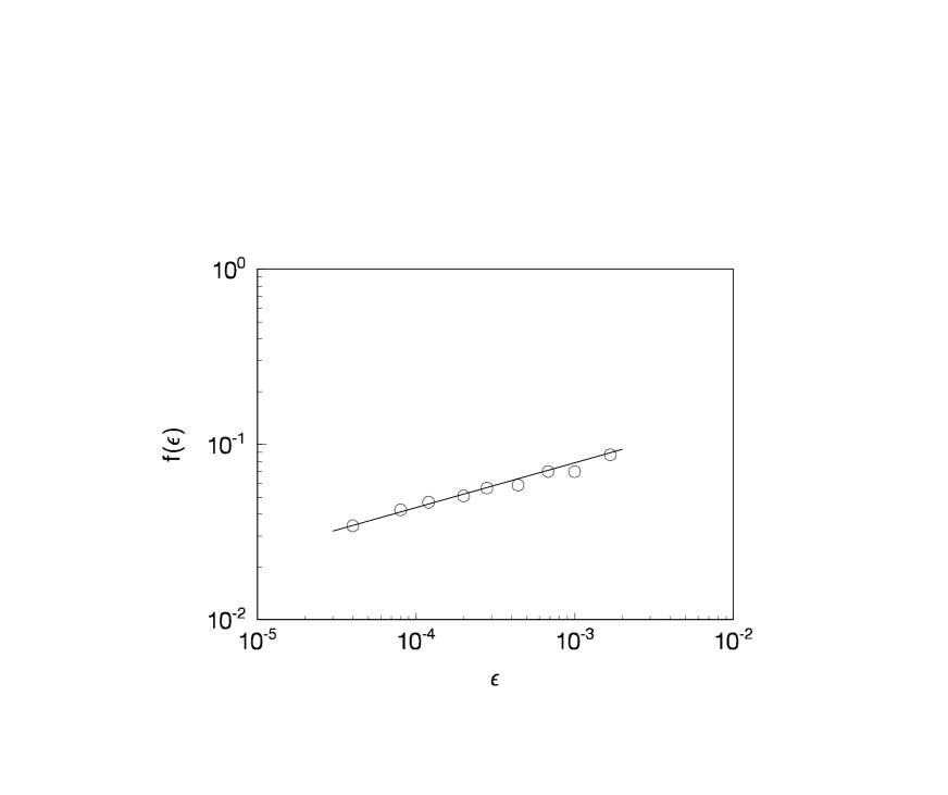
FIG. 7.: Scaling Law of the Singular Set.

FIG. 8.: Stroboscopic map a) in plane $(x,v_{x})$, b) in plane $(z,v_{z})$ for 5000 trajectories originating asymptotically at $X=0,v_{x}\in(-0.5,0.5)$ and $Z=150,v_{z}\in(-2,0)$.

REFERENCES

- [1] G.G.Paulus, W.Nicklich, Huale Xu, P.Lambropoulos and H.Walther, Phys. Rev. Lett. 72, 2851 (1994); B.Yang, K.J.Schafer, B.Walker, K.C.Kulander, P.Agostini, and L.F.DiMauro, Phys. Rev. Lett. 71, 3770 (1993)
- [2] P.B.Corkum, Phys. Rev. Lett. 71, 1994 (1993)
- [3] J.L.Krause, K.J.Schafer and K.C.Kulander, Phys.Rev.Lett. 68, 3535 (1992)
- [4] W.Becker, A.Lohr, and M.Kleber, J.Phys.B 27 ,L325 (1994)
- [5] Dehai Bao , Shi-Gang Chen and Jie Liu, Applied Phys. B 62 , 313 (1996)
- [6] M.Lewenstein, et al, Phys. Rev. A 51, 1495 (1995)
- [7] G.G.Paulus, W.Becker, W.Nicklich, and H.Walther, J.Phys.B 27, L703 (1994)
- [8] L.D.Landau, and E.M.Lifshitz, ’Quantum Mechanics’, P293 (1977), Pergamon Press
- [9] M.V.Ammosov, N.B.Delone and V.P.Krainov, Zh.Eksp.Teor.Fiz., 91, 2008 (1986)
- [10] N.B.Delone, and V.P.Krainov, J.Opt.Soc.Am.B 8 No.6, 1207, (1991)
- [11] J.G.Leopold and I.C.Percival, J.Phys.B 12, 709 (1979) J.Phys.B. 28 L109 (1995)
- [12] S.Brabec et al , Phys. Rev. A 54 , R2551 (1996)
- [13] B.Walker, B.Sheehy, K.C.Kulander, and L.F.DiMauro, Phys. Rev. Lett. 77, 5031 (1996)
- [14] G.G.Paulus, W.Nicklich, and H.Walther, Europhys. Lett. 27 267 (1994)
- [15] E.Doron, U.Smilansky, and A.Frenkel, Quantum Chaotic Scattering and Microwave Experiments in Quantum Chaos, ”Enrico Fermi” (1991), edited by G.Casati, I.Guarneri, and U.Smilansky, North-Holland (1993).
- [16] Edward Ott, ’Chaos in Dynamical System’,P174, Cambridge Univ. Press, (1993)
- [17] H.Friedrich and D.Wintgen, Phys.Rep. 183, 37 (1989)
- [18] G.Casati, B.V.Chirikov, D.L.Shepelyansky, and I.Guarneri, Phys.Rep. 154, 78 (1987)