Failure of linear control in noisy coupled map lattices

Abstract

We study a 1D ring of diffusively coupled logistic maps in the vicinity of an unstable, spatially homogeneous fixed point. The failure of linear controllers due to additive noise is discussed with the aim of clarifying the failure mechanism. A criterion is suggested for estimating the noise level that can be tolerated by the given controller. The criterion implies the loss of control for surprisingly low noise levels in certain cases of interest, and accurately accounts for the results of numerical experiments over a broad range of parameter values. Previous results of Grigoriev et al. (Phys. Rev. Lett. 79, 2795) are reviewed and compared with our numerical and analytic results.

I Introduction

Over the past several years, work on the feedback stabilization of periodic orbits in nonlinear dynamical systems has heightened interest within the physics community in the characteristics of various types of feedback-controlled systems. A problem of particular importance to physicists is the stabilization of uniform or ordered states in spatially extended systems, and it is of interest to analyze generic models of such systems and elucidate the features that make control difficult. Two recent articles have examined what is arguably the simplest representation of a spatially extended system with an unstable, homogeneous fixed point — a 1D ring of diffusively coupled logistic maps [1, 2]. This paper extends those analyses with the aim of clarifying the mechanism responsible for the failure of linear control in the presence of additive noise. Though more rigorous mathematical techniques of the theory of robust control can be applied to this problem to address specific engineering objectives [3], the following analysis provides a useful conceptual picture of the behavior that can be expected to be quantitatively accurate for generic physical systems.

Following Grigoriev et al. [2], we consider the feedback control of a ring of diffusively coupled maps with additive white noise:

$$z_{i}^{(t+1)}=f\left(z_{i}^{(t)}+\epsilon(z_{i-1}^{(t)}-2z_{i}^{(t)}+z_{i+1}^{(t)})\right)+\eta_{i}^{(t)},$$ (1)

where subscripts indicate spatial position and superscripts in parentheses indicate temporal iterates. (Throughout this paper superscripts without parentheses will indicate exponents.) For a given ring size, we show how a typical controller designed using standard linear-quadratic control theory may fail in the presence of very low noise levels, and we suggest a criterion for estimating the maximum tolerable noise level. For a fixed noise level, the maximum ring size that can be controlled can be taken as an estimate of the maximum allowable spacing between controllers in a much larger ring.

The noise $\eta_{i}^{(t)}$ is taken to be an independent number between $-\sqrt{3}\sigma$ and $\sqrt{3}\sigma$, so we have

$$\left\langle\eta_{i}^{(t)}\right\rangle = 0\quad\forall i,t$$ (2)

$$\left\langle\eta_{i}^{(t)}\eta_{j}^{(s)}\right\rangle = \sigma^{2}\delta_{ij}\delta_{ts},$$ (3)

where $\langle\rangle$ represents an ensemble average. We take the ring to contain $L$ sites and the spatial index to run from $1$ to $L$, so $z_{0}$ is identified with $z_{L}$, and $z_{L+1}$ with $z_{1}$. For concreteness, we will take $f$ to be the logistic map

$$f(z)=\mu z(1-z),$$ (4)

where $\mu$ is a real parameter. Generalization of the results to other maps is straightforward.

For any positive $\mu$, Eq. (1) has a homogeneous fixed point solution $z_{i}=1-1/\mu\equiv z^{\ast}$. For $\mu>3$, the homogeneous solution continues to exist but is unstable to long wavelength fluctuations. To study the stability of this solution, we linearize the system in the vicinity of the fixed point. Letting $x_{i}^{(t)}=z_{i}^{(t)}-z^{\ast}$, we obtain

$${\bf x}^{(t+1)}={\bf A}\cdot{\bf x}^{(t)},$$ (5)

with

$${\bf A}=\alpha\left(\begin{array}[]{cccccc}1-2\epsilon&\epsilon&0&\cdots&0&\epsilon\\ \epsilon&1-2\epsilon&\epsilon&\ddots&\ddots&0\\ 0&\ddots&\ddots&\ddots&\ddots&\vdots\\ \vdots&\ddots&\ddots&\ddots&\ddots&0\\ 0&\ddots&\ddots&\epsilon&1-2\epsilon&\epsilon\\ \epsilon&0&\cdots&0&\epsilon&1-2\epsilon\end{array}\right),$$ (6)

where $\alpha=2-\mu$ is the Floquet multiplier of $f$ at the fixed point.

Grigoriev et al. have applied well-known methods to show that control can be achieved in this noiseless system for arbitrarily large $L$ with just two controllers placed at adjacent sites [2]. Taking the two sites to be $i=1$ and $i=L$, the controlled system in the linear regime is written as

$${\bf x}^{(t+1)}=({\bf A}-{\bf BK}){\bf\cdot x}^{(t)},$$ (7)

where ${\bf B}$ is a $2\times L$ matrix with $B_{11}=B_{2L}=1$ and all other elements 0, and ${\bf K}$ is a $L\times 2$ matrix determined by iterative solution of an appropriate Ricatti equation derived using standard techniques of linear-quadratic control theory [4, 5]. We emphasize that the control scheme requires that every site of the system be observed; the feedback signals at sites 1 and $L$ are formed from a linear combination of all the $x_{i}$’s on the most recent time step. The problem of determining the optimal configuration for local controllers that only receive local information is beyond the scope of this work.

Grigoriev et al. have also pointed out that arbitrarily low noise levels destroy the control for sufficiently large system sizes. In general, for any given noise level $\sigma$, the full nonlinear system will not be stabilized by the feedback of Eq. (7) for sufficiently large $L$, or for fixed $L$ and sufficiently large $\sigma$. As will be discussed below, the breakdown of control is caused solely by the fact that the linear-quadratic control theory based on Eq. (5) does not take account of the nonlinear terms in Eq. (1). Naively, one might expect that the nonlinear deviations would be of order $\sigma^{2}$ and hence never play an important role for small $\sigma$, but it turns out that the feedback matrix ${\bf BK}$ necessarily becomes increasingly singular with increasing $L$, leading to great amplification of the noise by the controller itself. The nonlinear deviations due to this amplified noise can be large compared to the original noise level. When this occurs, the nonlinear deviations themselves are amplified further by the controller and the system quickly “blows up”.

In the following, we first describe a method for calculating the amplification of the noise by the controller. We then present our explicit criterion for estimating the tolerable noise level and show that it compares well with the numerical data. Finally, we compare our estimate to a different one suggested by Grigoriev et al., pointing out the relative advantages and disadvantages of each.

II Noise Amplification

The amplification of noise by the controller is a purely linear effect due to the nonnormality of the eigenvectors of the matrix ${\bf A-BK}$. In a nonnormal system that is linearly stable about ${\bf x}=0$ small perturbations in some directions may lead to transient growth in $||{\bf x}||$ before the eventual exponential decay. If the degree of nonnormality is high and the relevant eigenvalues are not too close to being degenerate, one can obtain large transient amplifications of an initial perturbation. Trefethen has emphasized the destabilizing influence of nonlinearities on highly nonnormal systems [6, 7].

Nonnormality is intrinsic to the problem of controlling a spatially extended system using sparsely distributed actuators. It is intuitively obvious that a perturbation occuring far from any actuator will undergo transient growth before the feedback generated by the controller can propagate to the position where the control is needed. This transient growth in the controlled system can be accounted for only by the occurence of nonnormal eigenvectors in the problem. As this physical picture suggests, the nonnormal effects become increasingly important with increasing $L$ and a fixed number of controllers.

As discussed by Trefethen and others, a nonnormal matrix can be characterized by its $\epsilon$-pseudospectra, which can be used to place bounds on the size of the transient growth of initial deviations from the fixed point. We are not aware, however, of any analytic techniques for determining these pseudospectra and so turn instead to a straightforward calculation of the noise amplification, taking advantage of the assumed delta-function correlations in the noise.

For the system defined by Eq. (7), we define an amplification constant $\gamma$ by the equation

$$\lim_{T\rightarrow\infty}\left\langle\frac{1}{L}|{\bf x}^{(T)}|^{2}\right\rangle^{1/2}=\gamma\sigma.$$ (8)

Given an explicit form for the matrix ${\bf A}-{\bf BK}$, $\gamma$ can be computed as follows.

Let ${\bf M}\equiv{\bf A}-{\bf BK}$, let ${\bf e}_{(i)}$ be a normalized eigenvector of ${\bf M}$, where $1<i<L$, let ${\bf v}_{(i)}$ be the vector orthogonal to all of the ${\bf e}_{(j)}$ with $j\neq i$, normalized such that ${\bf v}_{(i)}\cdot{\bf e}_{(j)}=\delta_{ij}$, and let $\lambda_{(i)}$ be the eigenvalue associated with ${\bf e}_{(i)}$. Using $\eta$${}^{(t)}=\sum_{i}{\bf e}_{(i)}({\bf v}_{(i)}\cdot$$\eta$${}^{(t)})$ and noting that the eigenvalues and eigenvectors of ${\bf M}$ may be complex, the left hand side of Eq. (8) can be evaluated directly:

$$\left\langle\frac{1}{L}\left|{\bf x}^{(T)}\right|^{2}\right\rangle = \frac{1}{L}\left\langle\left|\sum_{t=0}^{T}{\bf M}^{t}\mbox{\boldmath$\eta$}^{(T-t)}\right|^{2}\right\rangle$$ (9)

$$= \frac{1}{L}\sum_{t=0}^{T}\sum_{s=0}^{T}\sum_{i=1}^{L}\sum_{j=1}^{L}(\lambda_{(i)})^{t}(\lambda_{(j)}^{\ast})^{s}\left({\bf e}_{(i)}\cdot{\bf e}_{(j)}^{\ast}\right)\left\langle({\bf v}_{(i)}\cdot\mbox{\boldmath$\eta$}^{(T-t)})({\bf v}_{(j)}^{\ast}\cdot\mbox{\boldmath$\eta$}^{(T-s)})\right\rangle.$$ (10)

Using Eqs. (2) and (3) to evaluate the ensemble average and performing the resulting geometric sum, we find

$$\lim_{T\to\infty}\left\langle\frac{1}{L}\left|{\bf x}^{(T)}\right|^{2}\right\rangle=\frac{\sigma^{2}}{L}\sum_{i=1}^{L}\sum_{j=1}^{L}\frac{1}{1-\lambda_{(i)}\lambda_{(j)}^{\ast}}\left({\bf e}_{(i)}\cdot{\bf e}_{(j)}^{\ast}\right)\left({\bf v}_{(i)}\cdot{\bf v}_{(j)}^{\ast}\right).$$ (11)

Comparing to Eq. (8) we find

$$\gamma=\left(\frac{1}{L}\sum_{i=1}^{L}\sum_{j=1}^{L}\frac{1}{1-\lambda_{(i)}\lambda_{(j)}^{\ast}}\left({\bf e}_{(i)}\cdot{\bf e}_{(j)}^{\ast}\right)\left({\bf v}_{(i)}\cdot{\bf v}_{(j)}^{\ast}\right)\right)^{1/2}.$$ (12)

The added noise of strength $\sigma$ produces fluctuations of magnitude $\gamma\sigma$ in the controlled linear system. Analytical estimation of $\gamma$ can be quite difficult, but exact numerical evaluation of $\gamma$ is straightforward, given an explicit form for ${\bf M}$.

Table I shows values of $\gamma$ computed for various $L$, $\mu$, and $\epsilon$, with ${\bf K}$ determined as described below. The table also shows the maximum magnitude eigenvalue $\lambda_{(1)}$ for each case, making it clear that $\gamma$ may be large even when all the $\lambda_{(i)}$’s are substantially less than unity. The largeness of $\gamma$ derives from the nonnormality of the ${\bf e}_{(i)}$’s, which results in large magnitudes of some of the ${\bf v}_{(i)}$’s. Again, the amplification of the noise is a purely linear effect directly attributable to the transient growth of initial perturbations in nonnormal systems.

It is important to note (though it may be obvious to some) that control never fails in the purely linear system with noise added. There can be no threshold above which the noise causes divergence, since in the purely linear system there is no scale that can determine such a threshold. Though the noise may be amplified substantially, it is always limited.

III Estimates of Tolerable Noise Levels

Given our exact computation of $\gamma$, we can now estimate the value of $\sigma$ above which control will be lost in the full nonlinear system. Noting that the control perturbations are designed for optimal stabilization of the linearized system, we are led to consider the effect of the deviations from the linear behavior due to nonlinear terms in the full equations. We make the ansatz that correlations in these nonlinear deviations may be neglected, and hence treat the nonlinear deviations as an additional source of noise in the linear system. We refer to the original noise of strength $\sigma$ as the “additive noise” and the deviations induced by nonlinearities as the “deviational noise” with strength $\sigma_{d}$.

The size of the fluctuations about the fixed point will be given approximately by

$$\Delta=\gamma\sqrt{\sigma^{2}+\sigma_{d}^{2}}.$$ (13)

But $\sigma_{d}$ itself is produced by the nonlinear terms generated by the fluctuations. For the logistic map, $\sigma_{d}$ is therefore of the order of $\mu\Delta^{2}$, so we have

$$\Delta=\gamma\sqrt{\sigma^{2}+\mu^{2}\Delta^{4}}.$$ (14)

This equation has a real solution for $\Delta$ if and only if

$$\sigma<\frac{1}{2\mu\gamma^{2}}.$$ (15)

For $\sigma$ larger than this bound, the deviational noise will exceed the additive noise, thereby generating even larger deviational noise and an exponential divergence in the size of the fluctuations. Thus we take Eq. (15) as our criterion for obtaining effective control.

We note three reasons that this estimate could fail in principle. First, the estimate assumes that the dominant nonlinearity encountered by the fluctuating system is quadratic (which is true in the system studied in this paper). If higher order nonlinearities become important before our criterion is saturated, control may be lost for smaller $\sigma$. Second, the estimate assumes that there are no correlations in the deviational noise, which is not strictly correct. Finally, it is possible that control would be lost for smaller $\sigma$ if the fluctuations are not distributed roughly evenly over the components of ${\bf x}$. If a single component dominates the sum in Eq. (12), for example, it would be inappropriate to divide by $L$ in determining the relevant size of the fluctuations.

For these reasons, it is necessary to investigate the accuracy of our estimate using numerical simulation of the full nonlinear system with additive noise. We have performed simulations on systems of size $L=10$ and $L=20$ for several different values of the parameters $\mu$ and $\epsilon$. For each set of parameters values, the feedback control matrix ${\bf K}$ was determined using standard methods of linear-quadratic control theory. [4, 5] With weight matrices defined as ${\bf Q}={\bf I}_{L\times L}$ and ${\bf R}={\bf I}_{2\times 2}$, ${\bf K}$ is obtained from the relation:

$${\bf K}=({\bf R}+{\bf B}^{\dagger}{\bf PB})^{-1}{\bf B}^{\dagger}{\bf PA},$$ (16)

where ${\bf P}$ is determined from the Ricatti equation:

$${\bf P}=({\bf Q}+{\bf A}^{\dagger}{\bf PA})-{\bf A}^{\dagger}{\bf PB}({\bf R}+{\bf B}^{\dagger}{\bf PB})^{-1}{\bf B}^{\dagger}{\bf PA},$$ (17)

Eq. (17) is solved using a simple iterative procedure until ${\bf P}$ converges according to the condition:

$$\frac{\sum_{i,j}|P^{(T+1)}_{i,j}-P^{(T)}_{i,j}|}{\sum_{i,j}|P^{(T+1)}_{i,j}|}<10^{-6}.$$ (18)

More stringent convergence conditions did not produce noticeable changes in ${\bf K}$.

Each run is started from the homogeneous initial condition $z_{i}=z^{\ast}$ for all sites $i$, and the full system with control is iterated 20,000 times. All computations (including the calculation of ${\bf K}$) are performed at a precision of 30 decimal digits. If control was lost during a run, the feedback mechanism quickly caused the values of $z_{i}$ to stray from the allowed range for the logistic map and resulted in the rapid divergence of $|z_{i}|$. Figs. 1–3 shows $\sigma_{\rm max}$, the maximal value of the noise strength that is effectively controlled, as a function of the coupling $\epsilon$ for 3 values of $\mu$. Our predictions of $\sigma_{\rm max}$ match the measured values well for each $\mu$, indicating that the criterion proposed in Eq. (15) captures the important physics of noise-induced loss of control.

IV Comparison to method of Grigoriev, et al.

Grigoriev et al. have studied this problem from a different perspective. They have developed an estimate for the noise level at which control fails based on an analysis of the controllability of the linear system supplemented by the assumption that the feedback signal applied cannot exceed a number of order unity [2].

Briefly put, Grigoriev et al.’s estimate relies on the well-known result that controllability of a noiseless linear system implies the possibility of directing the system from any arbitrary point in phase space to the desired fixed point within a number of steps equal to the number of degrees of freedom $L$ [4, 5]. This strict criterion is then adapted to the noisy case by assuming that the relevant points in phase space for which it must be possible to direct the system to the fixed point in $L$ steps are just those that can be generated by iterating the uncontrolled noisy system through $L$ steps. If no constraints are placed on the size of the control perturbations, the fact that the system is known to be controllable implies that this can always be done for the purely linear system, regardless of the strength of the noise. If the strength of the control perturbations are limited, however, return to the fixed point in $L$ steps will not be possible for sufficiently large noise strength.

In order to estimate the size of the control perturbations needed for the particular geometry of the system at hand, Grigoriev et al. make the plausible assumption that every perturbation which can affect the central site by the end of the $L$ iterations should be of the order of magnitude required to produce an effect of size $\lambda_{\rm max}^{L}\sigma$ after propagating to the central site, where $\lambda_{\rm max}$ is the largest eigenvalue of ${\bf A}$. The last perturbation that can propagate to the central site by the end of the $L$ steps occurs at step $L/2$ and is suppressed (or amplified) by a factor $(\alpha\epsilon)^{L/2}$ before reaching the central site. Letting the size of the perturbation be $u$, we then have a necessary condition for effective control: we must permit $u$ large enough such that

$$u(\alpha\epsilon)^{L/2}=\lambda_{\rm max}^{L}\sigma.$$ (19)

The estimate of the maximal $\sigma$ that can be controlled is then given by the criterion that both $u$ and $u(\alpha\epsilon)^{L/2}$ remain less than unity. This argument leads directly to the criteria published in Ref. [2]. Note that for the system of coupled logistic maps, it is not clear from this analysis whether the restriction that control perturbations must not exceed order unity arises due to the fact that the individual maps diverge rapidly for $x$ outside the unit interval or due to the fact that nonlinear effects become important. The analysis presented in Section III above clearly indicates that it is the latter effect that is most important.

The method based on controllability has one great advantage over ours in that it makes no reference to the matrix ${\bf K}$; it is intended to apply to the optimal choice of ${\bf K}$, which may be different from the one determined above. One cannot rule out, for example, the possibility that a different choice of ${\bf K}$ would permit control of significantly higher noise levels.

The price of the generality of the method is inaccuracy in certain classes of systems. As shown in Figs. 1–3, for example, the prediction of Grigoriev et al. substantially underestimates the noise level that can be tolerated for small values of the coupling. For $\epsilon>0.5$, however, the prediction of Grigoriev, et al. tends to overestimate the maximum controllable noise strength.

The estimate of Grigoriev et al. handles the linear aspects of the problem quite elegantly but uses a rather crude estimate of when the nonlinear effects become important. It is possible for the deviational noise due to the nonlinearity to become important for much lower additive noise strengths than those required to force control perturbations of order unity. By directly computing the amplification of the noise by a specific proposed controller, we arrive at a more accurate estimate of the point at which nonlinear effects will become important and thereby invalidate the linear analysis. Note that the loss of control has nothing to do with the inability of the controller to supply sufficiently large perturbations, as might be suggested by the use of a cutoff of unity for the feedback signals in the analysis of Grigoriev, et al. Nor is it correct to estimate the importance of the nonlinear effects simply by comparing the magnitudes of linear and nonlinear terms on a single iteration. Rather, the loss of control is due to the effect described in Section III above, and occurs for feedback levels much lower than unity.

We view our results as complementary to those of Grigoriev et al., both for practical and conceptual reasons. Taken together, they form a coherent picture of the breakdown of control in a spatially extended homogeneous system. The important conceptual points can be summarized as follows: (1) sparsely distributed controllers in such systems give rise to highly nonnormal eigenvectors in the vicinity of a homogeneous fixed point; (2) this induces a large amplification of both the noise and the nonlinear deviations from the linearized systems; and (3) an accurate estimate of the tolerable noise level for a given implementation of feedback control can be obtained by considering the nonlinear effects as an additional source of noise and applying the criterion of Eq. (15).

$\mu$	$\epsilon$	$L$	$\gamma$	$|\lambda_{(1)}|$
3.5	0.30	10	1122.	0.807
3.5	0.50	10	412.	0.796
3.5	0.70	10	21427.	0.826
3.3	0.30	20	328814.	0.915
3.3	0.50	20	31615.	0.906
3.3	0.70	20	6.79 $\times 10^{8}$	0.886
3.1	0.30	20	3362.	0.953
3.1	0.50	20	1174.	0.945
3.1	0.50	20	5.98 $\times 10^{7}$	0.946

TABLE I.: The amplification factor $\gamma$ and the maximum magnitude eigenvalue $\lambda_{(1)}$ for a representative set of parameters $\mu$, $\epsilon$, and $L$.

FIG. 1.: The measured value, the prediction of Eq. (15), and the prediction of Grigoriev, et al. for the maximal noise strength $\sigma_{\rm max}$ for which control can be achieved for $\mu=3.1$ and $L=20$.

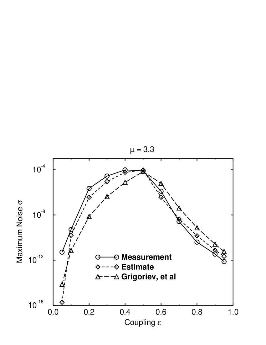
FIG. 2.: The measured value, the prediction of Eq. (15), and the prediction of Grigoriev, et al. for the maximal noise strength $\sigma_{\rm max}$ for which control can be achieved for $\mu=3.3$ and $L=20$.

FIG. 3.: The measured value, the prediction of Eq. (15), and the prediction of Grigoriev, et al. for the maximal noise strength $\sigma_{\rm max}$ for which control can be achieved for $\mu=3.5$ and $L=10$.