Quantum Mechanics and Semiclassics of Hyperbolic n-Disk Scattering Systems

Abstract

The scattering problems of a scalar point particle from an assembly of $1<n<\infty$ non-overlapping and disconnected hard disks, fixed in the two-dimensional plane, belong to the simplest realizations of classically hyperbolic scattering systems. Their simplicity allows for a detailed study of the quantum mechanics, semiclassics and classics of the scattering. Here, we investigate the connection between the spectral properties of the quantum-mechanical scattering matrix and its semiclassical equivalent based on the semiclassical zeta-function of Gutzwiller and Voros. We construct the scattering matrix and its determinant for any non-overlapping $n$-disk system (with $n<\infty$) and rewrite the determinant in such a way that it separates into the product over $n$ determinants of 1-disk scattering matrices – representing the incoherent part of the scattering from the $n$-disk system – and the ratio of two mutually complex conjugate determinants of the genuine multiscattering matrix ${\bf M}$ which is of Korringa-Kohn-Rostoker-type and which represents the coherent multidisk aspect of the $n$-disk scattering. Our quantum-mechanical calculation is well-defined at every step, as the on-shell T–matrix and the multiscattering kernel ${\bf M}\mbox{$-$}{\bf 1}$ are shown to be trace-class. The multiscattering determinant can be organized in terms of the cumulant expansion which is the defining prescription for the determinant over an infinite, but trace-class matrix. The quantum cumulants are then expanded by traces which, in turn, split into quantum itineraries or cycles. These can be organized by a simple symbolic dynamics. The semiclassical reduction of the coherent multiscattering part takes place on the level of the quantum cycles. We show that the semiclassical analog of the $m$th quantum cumulant is the $m$th curvature term of the semiclassical zeta function. In this way quantum mechanics naturally imposes the curvature regularization structured by the topological (not the geometrical) length of the pertinent periodic orbits onto the semiclassical zeta function. However, since the cumulant limit $m\to\infty$ and the semiclassical limit, $\hbar\to 0$ or (wave number) $k\to\infty$, do not commute in general, the semiclassical analog of the quantum multiscattering determinant is a curvature expanded semiclassical zeta function which is truncated in the curvature order. We relate the order of this truncation to the topological entropy of the corresponding classical system. We show this explicitly for the 3-disk scattering system and discuss the consequences of this truncation for the semiclassical predictions of the scattering resonances. We show that, under the above mentioned truncations in the curvature order, unitarity in $n$-disk scattering problems is preserved even at the semiclassical level. Finally, with the help of cluster phase shifts, it is shown that the semiclassical zeta function of Gutzwiller and Voros has the correct stability structure and is superior to all the competitor zeta functions studied in the literature.
PACS numbers: 03.65.Sq, 03.20.+i, 05.45.+b

1 Introduction

The main focus of this manuscript is on the transition from quantum mechanics to semiclassics in classically hyperbolic scattering systems, and in particular, on the convergence problems of periodic orbit expansions of $n$-disk repellers.

1.1 Motivation and historic perspective

Why more than 70 years after the birth of textbook quantum mechanics and in the age of supercomputers is there still interest in semiclassical methods? First of all, there remains the intellectual challenge to derive classical mechanics from quantum mechanics, especially for classically non-separable chaotic problems. Pure quantum mechanics is linear and of power-law complexity, whereas classical mechanics is generically of exponential complexity. How does the latter emerge from the former? Secondly, in many fields (atomic physics, molecular physics and quantum chemistry, but also optics and acoustics which are not quantum systems but are also characterized by the transition from wave dynamics to ray dynamics) semiclassical methods have been very powerful in the past and are still useful today for practical calculations, from the detection of elementary particles to the (radar)-detection of airplanes or submarines. Third, the numerical methods for solving multidimensional, non-integrable quantum systems are generically of “black-box” type, e.g. the diagonalization of a large, but truncated hamiltonian matrix in a suitably chosen basis. They are computationally intense and provide little opportunity for learning how the underlying dynamics organizes itself. In contrast, semiclassical methods have a better chance to provide an intuitive understanding which may even be utilized as a vehicle for the interpretation of numerically calculated quantum-mechanical data.

In the days of “old” quantum mechanics semiclassical techniques provided of course the only quantization techniques. Because of the failure, at that time, to describe more complicated systems such as the helium atom (see, however, the resolution of Wintgen and collaborators [1]; [2] and also [3] provide for a nice account of the history), they were replaced by modern quantum mechanics based on wave mechanics. Here, through WKB methods, they reappeared as approximation techniques for 1-dimensional systems and, in the generalization to the Einstein-Brillouin-Keller (EBK) quantization, for separable problems [3, 4, 5] where an $n$-degree-of-freedom system reduces to $n$ one-degree-of-freedom systems. Thus semiclassical methods had been limited to such systems which are classically nearly integrable.

It was Gutzwiller who in the late 60s and early 70s (see e.g. [5] and [6]) (re-)introduced semiclassical methods to deal with multidimensional, non-integrable quantum problems: with the help of Feynman path integral techniques the exact time-dependent propagator (heat kernel) is approximated, in stationary phase, by the semiclassical Van-Vleck propagator. After a Laplace transformation and under a further stationary phase approximation the energy-dependent semiclassical Green’s function emerges. The trace of the latter is calculated and reduces under a third stationary phase transformation to a smooth Weyl term (which parametrizes the global geometrical features) and an oscillating sum over all periodic orbits of the corresponding classical problem. Since the imaginary part of the trace of the exact Green’s function is proportional to the spectral density, the Gutzwiller trace formula links the spectrum of eigen-energies, or at least the modulations in this spectrum, to the Weyl term and the sum over all periodic orbits. Around the same time, Balian and Bloch obtained similar results with the help of multiple-expansion techniques for Green’s functions, especially in billiard cavities, see e.g. [7].

For more than one degree of freedom, classical systems can exhibit chaos. Generically these are, however, non-hyperbolic classically mixed systems with elliptic islands embedded in chaotic zones and marginally stable orbits for which neither the Gutzwiller trace formula nor the EBK-techniques apply, see Berry and Tabor [8]. Purely hyperbolic systems with only isolated unstable periodic orbits are the exceptions. But in contrast to integrable systems, they are generically stable against small perturbations [5]. Moreover, they allow the semiclassical periodic orbit quantization which can even be exact as for the case of the Selberg trace formula which relates the spectrum of the Laplace-Beltrami operator to geodesic motion on surfaces of constant negative curvature [9]. The Gutzwiller trace formula for generic hyperbolic systems is, however, only an approximation, since its derivation is based on several semiclassical saddle-point methods as mentioned above.

In recent years, mostly driven by the uprise of classical chaos, there has been a resurgence of semiclassical ideas and concepts. Considerable progress has been made by applying semiclassical periodic orbit formulae in the calculation of energy levels for bound-state systems or resonance poles for scattering systems, e.g., the anisotropic Kepler problem [5], the scattering problem on hard disks [10, 11, 12, 13, 14, 15], the helium atom [1] etc. (See Ref.[16] for a recent collection about periodic orbit theory.) It is well known that the periodic orbit sum for chaotic systems is divergent in the physical region of interest. This is the case on the real energy axis for bounded problems and in the region of resonances for scattering problems, because of the exponentially proliferating number of periodic orbits, see [5, 17]. Hence refinements have been introduced in order to transform the periodic orbit sum in the physical domain of interest to a still conditionally convergent sum by using symbolic dynamics and the cycle expansion [18, 19, 14], Riemann-Siegel lookalike formal and pseudo-orbit expansions [20, 21], surface of section techniques [22, 23], inside-outside duality [24], heat-kernel regularization [3, 25] etc. These methods tend to be motivated from other areas in physics and mathematics [26] such as topology of flows in classical chaos, the theory of the Riemann zeta functions, the boundary integral method for partial differential equations, Fredholm theory (see also [27]), quantum field theory etc.

In addition to the convergence problem, there exists the further complication for bounded smooth potential and billiard problems that the corresponding periodic orbit sums predict in general non-hermitean spectra. This problem is addressed by the Berry-Keating resummation techniques [20, 21] – however, in an ad-hoc fashion. In contrast, scattering problems circumvent this difficulty altogether since their corresponding resonances are complex to start with. Moreover, the scattering resonances follow directly from the periodic orbit sum, as the Weyl term is absent for scattering problems. In fact, it is more correct to state that the Weyl term does not interfer with the periodic sum, as a negative Weyl term might still be present, see e.g.[17]. Furthermore, scattering systems allow for a nice interpretation of classical periodic sums in terms of survival probabilities [2, 28]. In this respect, it is an interesting open problem why these classical calculations do not seem to generate a Weyl term, whether applied for bounded or scattering systems. For these reasons, the study of periodic sums for scattering systems should be simpler than the corresponding study for bound-state problems, as only the convergence problem is the issue.

1.2 The $n$-disk repeller: a model for hyperbolic scattering

Hence, one should look for a simple classically hyperbolic scattering system which can be used to address the convergence problem. It should not be too special, as for example the motion on a surface of constant curvature, but reasonably realistic and instructive. Eckhardt [10] suggested such a system, the “classical pinball machine”. It consists of a point particle and a finite number (in his case three) identical non-overlapping disconnected circular disks in the plane which are centered at the corners of a regular polygon (in his case an equilateral triangle). The point particle scatters elastically from the disks and moves freely in between collisions. The classical mechanics, semiclassics and quantum mechanics of this so-called three-disk system was investigated in a series of papers by Gaspard and Rice, [11, 12, 13], and, independently, by Cvitanović and Eckhardt [14], see also Scherer [17] and Ref.[15]. It belongs to a class of mechanical systems which are everywhere defocusing, hence no stable periodic orbit can exist (see Fig.1.1).

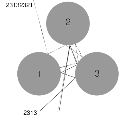
Figure 1.1: The three-disk repeller with the symbolic dynamics of the full domain. The figure is from Ref.[2].

The classical dynamics with one or two disks is simple, there is either no or one trapped trajectory. The latter is obviously unstable, since a small displacement leads to a defocusing after the reflection from the curved surface of disk [11]. The two-disk system is therefore one of the simplest hyperbolic scattering systems, but it is non-chaotic. However, with three or more disks there are infinitely many trapped trajectories forming a repeller [15]. The periodic orbits corresponding to these trapped trajectories are all isolated and unstable because of the defocusing nature of the reflections. Note that the one-disk and two-disk systems, although classically simple, are nonetheless interesting. The quantum-mechanical one-disk scattering system (since it is separable) has been one of the key models for building up the semiclassical theory of diffraction [29, 30, 31]. Similarly, the two-disk system became the toy ground for the periodic-orbit theory of diffraction [32, 33]. In fact, the two-disk system has infinitely many diffractive creeping periodic orbits which can be classified by symbolic dynamics similarly to the infinitely many geometrical orbits of the three-disk system. The symbolic dynamics of a general $n$-disk system is very simple, see e.g. [2]: periodic orbits can be classified by a series of “house numbers” of the disks which are visited by the point particle which follows the corresponding trajectory. Not all sequences are allowed: after each reflection from one disk, the point particle has to proceed to a different disk, since the evolution between the disk is the free one. Furthermore, for general geometries there may exist sequences which correspond to trajectories which would directly pass through a disk. The sequences corresponding to these so-called “ghost orbits” have to be excluded from the classical consideration. In summary, the geometrical periodic orbits (including ghost orbits) are labelled in the full domain of the $n$-disk repeller by itineraries (= periodic words) with $n$ different symbols (=letters) with the trivial “pruning” rule that successive letters in the itinerary must be different. The itineraries corresponding to ghost orbits have to be removed or “pruned” with all their sub-branches from the symbol tree. Periodic trajectories which have reflections from inside of a disk (i.e. the point particle traverses first through a disk and is then reflected from the other side of the disk) can be excluded from the very beginning. In fact, in our semiclassical reduction of Sec.5 we will show for all repeller geometries with $n$ non-overlapping disks that, to each specified itinerary, there belongs uniquely one standard periodic orbit which might contain ghost passages but which cannot be reflected from the inside. There is only one caveat: our method cannot decide whether grazing trajectories (which are tangential to a disk surface) belong to the class of ghost trajectories or to the class of reflected trajectories. For simplicity, we just exclude all geometries which allow for grazing periodic orbits from our proof. Alternatively, one might treat these grazing trajectories separately with the help of the diffractional methods of Refs.[31, 35].

The symbolic dynamics described above in the full domain applies of course to the equilateral three-disk system. However, because of the discrete ${\rm C}_{\rm 3v}$ symmetry of that system, the dynamics can be mapped into the fundamental domain (any one of the 1/6-th slices of the full domain which are centered at the symmetry-point of the system and which exactly cut through one half of each disk, see Fig.1.2).

Figure 1.2: Equilateral 3-disk system and its fundamental domain.

In this fundamental domain the three-letter symbolic dynamics of the full domain reduces a two-letter symbolic dynamics. The symbol ‘0’, say, labels all encounters of a periodic orbit with a disk in the fundamental domain where the point particle in the corresponding full domain is reflected to the disk where it was just coming from, whereas the symbol ‘1’, say, is reserved for encounters where the point particle is reflected to the other disk.

Whether the full or the fundamental domain is used, the 3-disk system allows for a unique symbolic labelling (if the disk separation is large enough even without non-trivial pruning). If a symbolic dynamics exist, the periodic orbits can be classified by their topological length which is defined as the length of the corresponding symbol sequence. In this case the various classical and semiclassical zeta functions are resummable in terms of the cycle expansion [18, 19] which can be cast to a sum over a few fundamental cycles (or primary periodic orbits) $t_{f}$ and higher curvature corrections $C_{m}$ of increasing topological order $m$:

$$\frac{1}{\zeta}=1-\sum_{f}t_{f}-\sum_{m}C_{m}\;.$$ (1.1)

The curvature $C_{m}$ in (1.1) contains all allowed periodic orbits of topological length $m$ for a specified symbolic dynamics and suitable “shadow-corrections” of combinations (pseudo-orbits) of shorter periodic orbits with a combined topological length $m$.

Common to most studies of the semiclassics of the $n$-disk repellers is that they are “bottom-up” approaches. Whether they use the Gutzwiller trace formula [5], the Ruelle or dynamical zeta function [36], the Gutzwiller-Voros zeta function [37], their starting point is the cycle expansion [18, 19, 28]. The periodic orbits are motivated from a semiclassical saddle-point approximation. The rest is classical in the sense that all quantities which enter the periodic orbit calculation as e.g. actions, stabilities and geometrical phases are determined at the classical level (see however Refs.[38, 39, 40] where leading $\hbar$-corrections to the dynamical zeta function as well as the Gutzwiller-Voros zeta function have been calculated). For instance, the dynamical zeta function has typically the form

$$\zeta_{0}^{-1}(E)=\prod_{p}(1-t_{p}),\quad t_{p}=\frac{1}{\sqrt{\Lambda_{p}}}\e^{({\rm i}/\hbar)S_{p}(E)-{\rm i}\frac{\pi}{2}\nu_{p}}.$$ (1.2)

The product is over all prime cycles (prime periodic orbits) $p$. The quantity $\Lambda_{p}$ is the stability factor of the $p$-th cycle, i.e., the expanding eigenvalue of the $p$-cycle Jacobian, $S_{p}$ is the action and $\nu_{p}$ is (the sum of) the Maslov index (and the group theoretical weight for a given representation) of the $p$-th cycle. For $n$-disk repellers, the action is simply $S_{p}=kL_{p}$, the product of the geometrical length $L_{p}$ of the periodic orbit and the wave number $k=\sqrt{2mE}$ in terms of the energy $E$ and mass $m$ of the point particle. The semiclassical predictions for the scattering resonances are then extracted from the zeros of the cycle-expanded semiclassical zeta-function. In this way one derives predictions of the dynamical zeta function for the leading resonances (which are the resonances closest to real $k$-axis). In the case of the Gutzwiller-Voros zeta function also subleading resonances result, however, only if the resonances lie above a line defined by the poles of the dynamical zeta function [41, 42, 43, 15]. The quasiclassical zeta function of Vattay and Cvitanović is entire and gives predictions for subleading resonances for the entire lower half of the complex plane [43].

1.3 Objective

As the $n$-disk scattering systems are generically hyperbolic, but still simple enough to allow for a closed-form quantum-mechanical setup [13] and detailed quantum-mechanical investigations [44, 45], we want to study the structure of the semiclassical periodic sum for a hyperbolic scattering system in a “top-down” approach, i.e. in a direct derivation from the exact quantum mechanics of the $n$-disk repeller. This is in contrast to the usual semiclassical “bottom-up” studies of the $n$-disk repellers which can be affected by uncontrolled operations during the long and mostly formal derivation from the Gutzwiller trace formula. Especially regularization prescriptions, like the cycle expansion, have to be added from the outside in order to get converging semiclassical predictions.

Hence, for any $n$-disk scattering problem with a finite number of non-overlapping disconnected disks we want to construct a direct link from the defining exact ${\bf S}$-matrix to the pertinent semiclassics (in terms of a suitable periodic-orbit expansion) with the following qualifications:

1. The derivation should lead to a unique specification of the periodic orbits for a given $n$-disk geometry. The method should be able to handle $n$-disk geometries which allow for ghost orbits, i.e., periodic orbits existing in any of the pertinent “parent” disk-systems (defined by the removal of one or more disks) which are blocked by the return of at least one of the removed disks.

2. Since disk-systems are known where the semiclassics is strongly governed by diffractive orbits (see [33] and especially [63] for the 2-dimensional scattering analog of the two-well-potential problem), diffractive periodic orbits should emerge together with their standard partners.

3. The subleading stability structure of the standard periodic orbits should follow from this derivation in order to discriminate between the Gutzwiller-Voros zeta function and other competitors, e.g., the dynamical zeta function of Ruelle [36] or the quasiclassical zeta function of Vattay and Cvitanović [43]; in other words, we want to derive the semiclassical spectral function.

4. The setup of the starting-point, the quantum-mechanical side, should not be plagued by formal or uncontrolled manipulations or assumptions. Especially, if the quantum-mechanical side does not exist without a suitable regularization prescription, the latter should be provided before the semiclassical reduction is performed. This should exclude that the semiclassical sums encounter hidden problems which are already present at the quantum-mechanical level.

5. The link between the exact quantum mechanics and semiclassics should not only allow for the computation of scattering resonance, but should be valid for all values of the wave number, also away from the resonances and from the real axis, modulo the boundary of semiclassical convergence, as this issue can only be addressed during the link-procedure. Branch cuts and singularities on the quantum-mechanical side have to be taken into account of course.

6. The spectral function should not only result in a formal sense, but, if necessary, with a pertinent regularization and summation prescription that should not be imposed from the outside.

7. Most importantly, the derivation should be well-defined and allow for a test of the summation prescription of the period-orbit expansion. If potential problems occur, they should be pinpointed in the derivation.

1.4 Outline

The manuscript is organized as follows. We begin in Sec.2 with the standard approach relating quantum-mechanical and semiclassical resonances for $n$-disk repellers.

Generalizing the work of Gaspard and Rice [13] to non-overlapping $n$-disk problems of arbitrary geometry and disk sizes we construct in Sec.3 the ${\bf S}$-matrix from stationary scattering theory. Details of this calculation are relegated to App.B. Utilizing the machinery of trace-class operators which are summarized in App.A we construct the determinant of the $n$-disk ${\bf S}$-matrix as the product of $n$ one-disk determinants and the ratio of the determinant and its complex conjugate of the genuine multiscattering matrix. It is shown how the latter determinants split under symmetry operations. The proofs for the existence of the determinants are relegated to App.C and the comparison to alternative formulations of the multiscattering kernel can be found in App.D.

In Sec.4 we state the link between the exact determinant of the $n$-disk ${\bf S}$-matrix and the Gutzwiller-Voros curvature expansion. We discuss the semiclassical limit of the incoherent part, whereas the actual calculation is reported in App.E. It is shown that, under the semiclassical reduction of the quantum traces, the Plemelj-Smithies recursion relation for the quantum cumulants transforms into the recursion relation for the semiclassical curvatures which are known from the cycle expansion.

The actual semiclassical reduction is worked out in Sec.5. We start with the construction of the quantum cycles or itineraries built from the convolution of a finite number of multiscattering kernels and show that they have the same symbolic dynamics in the full domain of an arbitrary $n$-disk system as their semiclassical counterparts, the geometrical periodic orbits. We discuss the case that the quantum-mechanical cumulant sum incorporates geometries which classically allow for non-trivial pruning and hence for periodic orbits which pass undisturbed straight through a disk, see Refs.[54, 49]. We show how these ghost orbits cancel against their “parent” periodic orbits resulting from itineraries without the disk which is affected by the ghost passage. For the general case of an arbitrary quantum cycle Sec.5.3 mirrors the semiclassical reduction of the convolution of two multiscattering kernels studied in detail in App.F with the help of the Watson contour integration and suitable deformations of the paths in the complex angular-momentum plane. In Sec.5.4 the geometrical limit of a quantum cycle is studied, which is generalized to the case of $r$ times repeated cycles in the following section. In Sec.5.6 the ghost cancellation rule for arbitrary cycles is derived. The semiclassical diffractive creeping contributions are constructed and studied in Secs.5.7 and 5.8. Sec.5 ends with the proof that an arbitrary quantum itinerary reduces semiclassically to a periodic orbit of Gutzwiller-Voros stability, such that the link between the exact determinant of the $n$-disk ${\bf S}$-matrix and the Gutzwiller-Voros curvature sum is established.

Numerical tests of the semiclassical curvature expansion can be found in Sec.6 for the example of the three-disk system in the ${\rm A}_{\rm 1}$ symmetry-class representation. First, the exact quantum-mechanical data are compared to the semiclassical predictions of the Gutzwiller-Voros zeta function, the dynamical zeta function [36] and the quasiclassical zeta function suggested in [43], where all three semiclassical zeta function are expanded in curvatures which are truncated at finite order. Secondly, the exact cluster phase shift (defined by the phase of the determinant of the multiscattering matrix) is compared with the semiclassical predictions of the three zeta functions. Although all three zeta functions seem at first sight empirically equivalent, as they all predict the same leading resonances closest to the real $k$-axis, this comparison shows clearly which of the three is superior and is hence the candidate for – at least – the FAPP (“for all practical purposes”) zeta function. Sec.6 ends with an order-by-order comparison of the exact cumulants with their semiclassical counterpart, the curvatures for the Gutzwiller-Voros zeta function. From these numerical data we extract an empirical truncation rule for the curvature expansion as a function of the wave number. We relate this rule to the uncertainty bound resulting from finite quantum-mechanical resolution of the exponentially proliferating details of the classically repelling set.

Sec.7 concludes with a summary. Here we emphasis the preservation of unitarity under the semiclassical reduction, the decoupling of the incoherent one-disk from the coherent $n$-disk determinants, and the particularities, when bounded domains are formed in the case of (nearly) touching disks. Furthermore, the resonance data are correlated with the truncation from the uncertainty bound. We discuss the relevance of those periodic orbits whose topological order exceeds the uncertainty bound. Arguments are presented that the Gutzwiller-Voros zeta function ought to be interpreted in the asymptotic sense as an truncated sum, whether it converges or not. The conclusions end with a discussion on $\hbar$ corrections.

Note that the contents of Apps.B and C are based on M. Henseler’s diploma thesis [46], while Sec.6 as well as Secs.3,4 and Apps.A.1-2 have partial overlap with Refs.[47] and [48], respectively.

2 Semiclassical resonances of the $n$-disk system

The connection between exact quantum mechanics, on the one side, and semiclassics, on the other, for the $n$-disk repellers in the standard “bottom-up” approach, is rather indirect. It has been mainly based on a comparison of the exact and semiclassical predictions for resonance data. In the exact quantum-mechanical calculations the resonance poles are extracted from the zeros of a characteristic scattering determinant (see ref. [13] and below), whereas the semiclassical predictions follow from the zeros (poles) of one of the semiclassical zeta functions. These semiclassical quantities have either formally been taken over from bounded problems (where the semiclassical reduction is performed via the spectral density) [17, 15] or they have just been extrapolated from the corresponding classical scattering determinant [42, 43]. Our aim is to construct a direct link between the quantum-mechanical and semiclassical treatment of hyperbolic scattering in a concrete context, the $n$-disk repellers.

Following the methods of Gaspard and Rice [13] we will construct in Sec.3 and App.B the pertinent on-shell T–matrix which splits into the product of three matrices, namely ${\bf C}(k){\bf M}^{-1}(k){\bf D}(k)$. The matrices ${\bf C}(k)$ and ${\bf D}(k)$ couple the incoming and outgoing scattering wave (of wave number $k$), respectively, to one of the disks, whereas the matrix ${\bf M}(k)$ parametrizes the scattering interior, i.e., the multiscattering evolution in the multidisk geometry. The understanding is that the resonance poles of the $n>1$ disk problem can only result from the zeros of the characteristic determinant ${\rm det}{\bf M}(k)$; see the quantum-mechanical construction of Gaspard and Rice [13] for the three-disk scattering system [10, 11, 14]. Their work refers back to Berry’s application [49, 50] of the Korringa-Kohn-Rostoker (KKR) method [51] to the (infinite) two-dimensional Sinai-billiard problem which, in turn, is based on Lloyd’s multiple scattering method [52, 53] for a finite cluster of non-overlapping muffin-tin potentials in three dimensions.

The resonance poles are calculated numerically by solving ${\rm det}{\bf M}(k)=0$ in a finite, but large basis, such that the result is insensitive to an enlargement of the basis (see, e.g., [44]). On the semiclassical side, the geometrical primitive periodic orbits (labelled by $p$) have been summed up – including repeats (labelled by $r$) – in the Gutzwiller-Voros zeta function [5, 37]

$$Z_{\rm GV}(z;k) = \exp\left\{-\sum_{p}\sum_{r=1}^{\infty}\frac{1}{r}\frac{\left(z^{n_{p}}\,t_{p}(k)\right)^{r}}{1-\frac{1}{\Lambda_{p}^{r}}}\right\}$$ (2.1)

$$= \prod_{p}\prod_{j=0}^{\infty}\left(1-\frac{z^{n_{p}}t_{p}(k)}{{\Lambda_{p}}^{j}}\right)$$

the dynamical zeta function of Ruelle [36]

$$\zeta_{0}^{-1}(z;k)=\exp\left\{-\sum_{p}\sum_{r=1}^{\infty}\frac{1}{r}z^{rn_{p}}\,t_{p}(k)^{r}\right\}=\prod_{p}\left(1-z^{n_{p}}t_{p}\right)$$ (2.2)

(which is the $j=0$ part of the Gutzwiller-Voros zeta function) or the quasiclassical zeta function of Vattay and Cvitanović [43]

$$Z_{\rm qcl}(z;k) = \exp\left\{-\sum_{p}\sum_{r=1}^{\infty}\frac{1}{r}\frac{\left(z^{n_{p}}\,t_{p}(k)\right)^{r}}{\left(1-\frac{1}{\Lambda_{p}^{r}}\right)^{2}\left(1-\frac{1}{\Lambda_{p}^{2r}}\right)}\right\}$$ (2.3)

$$= \prod_{p}\prod_{j=0}^{\infty}\prod_{l=0}^{\infty}\left(1-\frac{z^{n_{p}}t_{p}(k)}{\Lambda_{p}^{\,j+2l}}\right)^{j+1}\;$$

which is an entire function. In all cases $t_{p}(k)=\e^{{\rm i}kL_{p}-{\rm i}\nu_{p}\pi/2}/\sqrt{|\Lambda_{p}|}$ is the so-called $p^{\,\rm th}$ cycle, $n_{p}$ is its topological length and $z$ is a book-keeping variable for keeping track of the topological order. The input is purely geometrical, i.e., the lengths $L_{p}$, the Maslov indices $\nu_{p}$, and the stabilities (the leading eigenvalues of the stability matrices) $\Lambda_{p}$ of the $p^{\,\rm th}$ primitive periodic orbits. Note that both expressions for the three zeta functions, either the exponential one or the reformulation in terms of infinite product(s), are purely formal. In the physical region of interest, they may not even exist without regularization. (An exception is the non-chaotic 2-disk system, as it has only one periodic orbit, $t_{0}(k)$.) Therefore, the semiclassical resonance poles are computed from these zeta functions in the curvature expansion [42, 19, 15] up to a given topological length $m$. This procedure corresponds to a Taylor expansion of, e.g., $Z_{\rm GV}(z;k)$ in $z$ around $z=0$ up to order $z^{m}$ (with $z$ set to unity in the end), e.g.,

$$Z_{\rm GV}(z;k) = z^{0}-z\sum_{n_{p}=1}\frac{t_{p}}{1-\frac{1}{\Lambda_{p}}}$$

$$\mbox{}-\frac{z^{2}}{2}\left\{\sum_{n_{p}=2}\frac{2t_{p}}{1-\frac{1}{\Lambda_{p}}}\mbox{}+\sum_{n_{p}=1}\frac{(t_{p})^{2}}{1-\left(\frac{1}{\Lambda_{p}}\right)^{2}}-\sum_{n_{p}=1}\sum_{n_{p^{\prime}}=1}\frac{t_{p}}{1-\frac{1}{\Lambda_{p}}}\frac{t_{p^{\prime}}}{1-\frac{1}{\Lambda_{p^{\prime}}}}\right\}+\cdots\;.$$

The hope is that the limit $m\to\infty$ exists — at least in the semiclassical regime ${\rm Re}\,k\gg 1/a$ where $a$ is the characteristic length of the scattering potential. We will show below that in the quantum-mechanical analog — the cumulant expansion – this limit can be taken, but that there are further complications in in the semiclassical case.

The cycle expansion is one way of regularizing the formal expression of the Gutzwiller-Voros zeta function (2.1). Another way would be the multiplication with a smooth cutoff function, as it is customary in quantum field theories, see e.g. [3]. This is, in principle, allowed. In order to be able to compare quantum mechanics with semiclassics, however, the very same cutoff function has to be introduced already on the quantum level. Candidates for such cutoff functions which work on the quantum side and on the semiclassical side are not so obvious, see e.g. App.A.4. They have to be formulated in terms of the ${\bf T}$-matrix or the multiscattering kernel and would introduce further complications. Fortunately, the quantum-mechanical side of the present problem exists without further regularization. Thus there is no need for an extra cutoff function.

As mentioned above, the connection between quantum mechanics and semiclassics for these scattering problems has been the comparison of the corresponding resonance poles, the zeros of the characteristic determinant on the one side and the zeros of the Gutzwiller-Voros zeta function or its competitors – in general in the curvature expansion – on the other side. In the literature (see, e.g., Refs.[12, 17, 15] based on Ref.[54] or [55]) the link is motivated by the semiclassical limit of the left hand sides of the Krein-Friedel-Lloyd sum for the (integrated) spectral density [56, 57] and [52, 53]

$$\lim_{\epsilon\to+0}\lim_{b\to\infty}\left(N^{(n)}(k+{\rm i}\epsilon;b)-N^{(0)}(k+{\rm i}\epsilon;b)\right) = \frac{1}{2\pi}{\rm Im}{\rm Tr}\ln{\bf S}(k)\ ,$$ (2.5)

$$\lim_{\epsilon\to+0}\lim_{b\to\infty}\left(\rho^{(n)}(k+{\rm i}\epsilon;b)-\rho^{(0)}(k+i\epsilon;b)\right) = \frac{1}{2\pi}{\rm Im}{\rm Tr}\frac{d}{dk}\ln{\bf S}(k)\;.$$ (2.6)

See also Ref.[58] for a modern discussion of the Krein-Friedel-Lloyd formula and Refs.[55, 59] for the connection of (2.6) to the the Wigner time delay. In this way the scattering problem is replaced by the difference of two bounded reference billiards (e.g. large circular domains) of the same radius $b$ which finally will be taken to infinity, where the first contains the scattering region or potentials, whereas the other does not (see Fig.2.1). Here $\rho^{(n)}(k;b)$ ($N^{(n)}(k;b)$) and $\rho^{(0)}(k;b)$ ($N^{(0)}(k;b)$) are the spectral densities (integrated spectral densities) in the presence or absence of the scatterers, respectively. In the semiclassical approximation, they will be replaced by a Weyl term and an oscillating sum over periodic orbits [5].

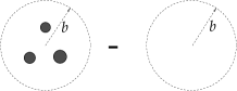
Figure 2.1: The “difference” of two bounded reference systems, where one includes the scattering system.

Note that this expression makes only sense for wave numbers above the real $k$-axis. Especially, if $k$ is chosen to be real, $\epsilon$ must be greater than zero. Otherwise, the exact left hand sides (2.5) and (2.6) would give discontinuous staircase or even delta function sums, respectively, whereas the right hand sides are continuous to start with, since they can be expressed by continuous phase shifts. Thus, the order of the two limits in (2.5) and (2.6) is essential, see e.g. Balian and Bloch [54] who stress that smoothed level densities should be inserted into the Friedel sums. In Ref.[12], chapter IV, Eqs. (4.1–4), the order is, however, erroneously inverted.

Our point is that this link between semiclassics and quantum mechanics is still of very indirect nature, as the procedure seems to use the Gutzwiller-Voros zeta function for bounded systems and not for scattering systems and as it does not specify whether and which regularization has to be used for the semiclassical Gutzwiller trace formula. Neither the curvature regularization scheme nor other constraints on the periodic orbit sum follow naturally in this way. For instance, as the link is made with the help of bounded systems, the question might arise whether even in scattering systems the Gutzwiller-Voros zeta function should be resummed à la Berry and Keating [21] or not. This question is answered by the presence of the ${\rm i}\epsilon$ term and the second limit. The wave number is shifted from the real axis into the positive imaginary $k$-plane. This corresponds to a “de-hermitezation” of the underlying exact hamiltonian – the Berry-Keating resummation should therefore not apply, as it is concerned with hermitean problems. The necessity of the $+{\rm i}\epsilon$ in the semiclassical calculation can be understood by purely phenomenological considerations: Without the ${\rm i}\epsilon$ term there is no reason why one should be able to neglect spurious periodic orbits which solely are there because of the introduction of the confining boundary. The subtraction of the second (empty) reference system helps just in the removal of those spurious periodic orbits which never encounter the scattering region. The ones that do would still survive the first limit $b\to\infty$, if they were not damped out by the $+{\rm i}\epsilon$ term.

Below, we will construct explicitly a direct link between the full quantum-mechanical S–matrix and the Gutzwiller-Voros zeta function. It will be shown that all steps in the quantum-mechanical description are well defined, as the T–matrix and the matrix ${\bf A}\equiv{\bf M}-{\bf 1}$ are trace-class matrices (i.e., the sum of the diagonal matrix elements is absolutely converging in any orthonormal basis). Thus the corresponding determinants of the S-matrix and the characteristic matrix M are guaranteed to exist, although they are infinite matrices.

3 The $n$-disk S-matrix and its determinant

Following the methods of Berry [49] and Gaspard and Rice [13] we here describe the elastic scattering of a point particle from $n$ hard disks in terms of stationary scattering theory. Because of the hard-core potential on the disk surfaces it turns into a boundary value problem. Let ${\psi}(\pol{r}\,)$ be a solution of the pertinent stationary Schrödinger equation at spatial position $\pol{r}$:

$$\left({\pol{\nabla}_{{r}}}^{2}+{\pol{k}}^{2}\right){\psi}(\pol{r}\,) = 0\;,\qquad\pol{r}\;\mbox{outside the $n$ disks,}$$

$$\psi(\pol{r}\,) = 0\;,\qquad\pol{r}\;\mbox{on the surfaces of the disks,}$$

where $E={\hbar^{2}}{\pol{k}^{2}}/2m$ is the energy of the point-particle written in terms of its mass $m$ and the wave vector $\pol{k}$ of the incident wave. After the wave function $\psi(\pol{r}\,)$ is expanded in a basis of angular momentum eigenfunctions in two dimensions, it reads

$$\psi(\pol{r}\,)=\sum_{m=-\infty}^{\infty}\psi_{m}^{k}(\pol{r}\,)\e^{{\rm i}m\frac{\pi}{2}}\e^{-{\rm i}m\Phi_{k}}\;,$$

where $k$ and $\Phi_{k}$ are the length and angle of the wave vector, respectively. The scattering problem in this basis reduces to

$$\left({\pol{\nabla}_{{r}}}^{2}+{\pol{k}}^{2}\right){\psi}^{k}_{m}(\pol{r}\,) = 0\;,\qquad\pol{r}\;\mbox{outside the disks;}$$

$$\psi^{k}_{m}(\pol{r}\,) = 0\;,\qquad\pol{r}\;\mbox{on the disk surfaces.}$$

For large distances from the scatterers ($kr\to\infty$) the spherical components $\psi_{m}^{k}$ can be written as a superposition of in-coming and out-going spherical waves,

$$\psi^{k}_{m}(\pol{r}\,)\sim\frac{1}{\sqrt{2\pi kr}}\sum_{m^{\prime}=-\infty}^{\infty}\left[\delta_{mm^{\prime}}\e^{-{\rm i}(kr-\frac{\pi}{2}m^{\prime}-\frac{\pi}{4})}+{\bf S}_{mm^{\prime}}\e^{{\rm i}(kr-\frac{\pi}{2}m^{\prime}-\frac{\pi}{4})}\right]\e^{{\rm i}m^{\prime}\Phi_{r}}\;,$$ (3.1)

where $r$ and $\Phi_{r}$ denote the distance and angle of the spatial vector $\pol{r}$ as measured in the global two-dimensional coordinate system. Eq.(3.1) defines the scattering matrix ${\bf S}$ which is unitary because of probability conservation. In the angular-momentum basis its matrix elements ${\bf S}_{mm^{\prime}}$ describe the scattering of an in-coming wave with angular momentum $m$ in an out-going wave with angular momentum $m^{\prime}$. If there are no scatterers, then ${\bf S}={\bf 1}$ and the asymptotic expression of the plane wave $\e^{{\rm i}\pol{k}\cdot\pol{r}}$ in two dimensions is recovered from $\psi(\pol{r}\,)$. All scattering effects are incorporated in the deviation of ${\bf S}$ from the unit matrix, i.e., in the T-matrix defined as ${\bf S}(k)={\bf 1}-{\rm i}{\bf T}(k)$. In general, S is non-diagonal and therefore non-separable. An exception is the one-disk problem (see below).

For any non-overlapping system of $n$ disks (of, in general, different disk-radii $a_{j}$, $j=1,\dots,n$) the $\bf S$-matrix can be further split up. Using the methods and notation of Gaspard and Rice [13] this is achieved in the following way (see also Ref.[53] and App. B for a derivation of this result):

$${\bf S}_{mm^{\prime}}^{(n)}(k) = \delta_{mm^{\prime}}-{\rm i}{\bf T}_{mm^{\prime}}^{(n)}(k)$$ (3.2)

$$= \delta_{mm^{\prime}}-{\rm i}{\bf C}_{ml}^{\ \ j}(k){\left({\bf M}^{-1}(k)\right)}_{ll^{\prime}}^{jj^{\prime}}{\bf D}_{l^{\prime}m^{\prime}}^{j^{\prime}}(k)\;.$$

Here the upper indices $j,\,j^{\prime}=1,\dots,n<\infty$ label the $n$ different disks, whereas the lower indices are the angular momentum quantum numbers. Repeated indices are summed over. The matrices ${\bf C}^{j}$ and ${\bf D}^{j}$ depend on the origin and orientation of the global coordinate system of the two-dimensional plane and are separable in the disk index $j$:

$${\bf C}_{ml}^{\ \ j} = \frac{2{\rm i}}{\pi a_{j}}\frac{J_{m-l}(kR_{j})}{H^{(1)}_{l}(ka_{j})}\e^{im\Phi_{R_{j}}}\;,$$ (3.3)

$${\bf D}_{l^{\prime}m^{\prime}}^{j^{\prime}} = -\pi a_{j^{\prime}}J_{m^{\prime}-l^{\prime}}(kR_{j^{\prime}})J_{l^{\prime}}(ka_{j^{\prime}})\e^{-{\rm i}m^{\prime}\Phi_{R_{j^{\prime}}}}\;,$$ (3.4)

where $R_{j}$ and $\Phi_{R_{j}}$ are the distance and angle, respectively, of the ray from the origin in the 2-dimensional plane to the center of disk $j$ as measured in the global coordinate system (see Fig.3.1). $H^{(1)}_{l}(kr)$ is the ordinary Hankel function of first kind and $J_{l}(kr)$ the corresponding ordinary Bessel function. The matrices ${\bf C}^{j}$ and ${\bf D}^{j}$ parameterize the coupling of the incoming and outgoing scattering waves, respectively, to the scattering interior at the $j^{\,\rm th}$ disk. Thus they describe only the single-disk aspects of the scattering of a point particle from the $n$ disks. The matrix ${\bf M}^{jj^{\prime}}$ has the structure of a Kohn-Korringa-Rostoker (KKR)-matrix, see Refs.[49, 50, 53],

$${\bf M}_{ll^{\prime}}^{jj^{\prime}}=\delta_{jj^{\prime}}\delta_{ll^{\prime}}+(1-\delta_{jj^{\prime}})\,\frac{a_{j}}{a_{j^{\prime}}}\,\frac{J_{l}(ka_{j})}{H^{(1)}_{l^{\prime}}(ka_{j^{\prime}})}\,H^{(1)}_{l-l^{\prime}}(kR_{jj^{\prime}})\,\Gamma_{jj^{\prime}}(l,l^{\prime})\;.$$ (3.5)

without Ewald resummation [49], as the number of disks is finite. Here $R_{jj^{\prime}}$ is the separation between the centers of the $j$th and $j^{\prime}$th disk and $R_{jj^{\prime}}=R_{j^{\prime}j}$, of course. The auxiliary matrix $\Gamma_{jj^{\prime}}(l,l^{\prime})=\e^{{\rm i}(l\alpha_{j^{\prime}j}-l^{\prime}(\alpha_{jj^{\prime}}-\pi))}$ contains – aside from a phase factor – the angle $\alpha_{j^{\prime}j}$ of the ray from the center of disk $j$ to the center of disk $j^{\prime}$ as measured in the local (body-fixed) coordinate system of disk $j$ (see Fig.3.1).

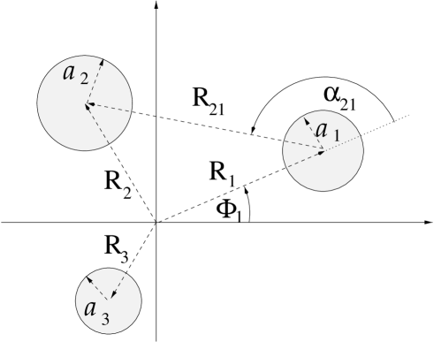
Figure 3.1: Global and local coordinates for a general $3$-disk problem.

Note that $\Gamma_{jj^{\prime}}(l,l^{\prime})=(-1)^{l-l^{\prime}}(\,\Gamma_{j^{\prime}j}(l^{\prime},l)\,)^{\ast}$. The “Gaspard and Rice prefactors” of $\bf M$, i.e., $(\pi a/2i)$ in [13], are rescaled into $\bf C$ and $\bf D$. The matrix ${\bf A}\equiv{\bf M}-{\bf 1}$ contains the genuine multidisk “scattering” aspects of the the $n$-disk problem, e.g., in the pure 1-disk scattering case, $\bf A$ vanishes. When $({\bf M}^{-1})^{jj^{\prime}}$ is expanded as a geometrical series about the unit matrix $\{\delta^{jj^{\prime}}\}$, a multiscattering series in “powers” of the matrix ${\bf A}$ is created.

The product ${\bf C}{\bf M}^{-1}{\bf D}$ is the on-shell ${\bf T}$-matrix of the $n$-disk system. It it the two-dimensional analog of the three-dimensional result of Lloyd and Smith for a finite cluster of non-overlapping muffin-tin potentials. At first sight the expressions of Lloyd and Smith (see Eq.(98) of [53] and also Berry’s form [49] for the infinite Sinai cluster) seem to look simpler than ours and the original ones of Ref.[13], as, e.g., in ${\bf M}$ the asymmetric term $a_{j}J_{l}(ka_{j})/a_{j^{\prime}}H^{(1)}_{l^{\prime}}(ka_{j^{\prime}})$ is replaced by a symmetric combination, $J_{l}(ka_{j})/H^{(1)}_{l}(ka_{j})$. Under a formal manipulation of our matrices we can derive the same result (see App. D). In fact, it can be checked that the (formal) cumulant expansion of Lloyd’s and our ${\bf M}$-matrix are identical and that also numerically the determinants give the same result. Note, however, that in Lloyd’s case the trace-class property of ${\bf M}$ is lost, such that the infinite determinant and the corresponding cumulant expansion converge only conditionally, and not absolutely as in our case. The latter fact is based on the trace-class properties of the underlying matrices and is an essential precondition for all further simplifications, as e.g. unitary transformations, diagonalization of the matrices, etc.

A matrix is called “trace-class”, if and only if, for any choice of the orthonormal basis, the sum of the diagonal matrix elements converges absolutely; it is called “Hilbert-Schmidt”, if the sum of the absolute squared diagonal matrix elements converges (see M. Reed and B. Simon, Vol.1 and 4 [60, 61] and App. A for the definitions and properties of trace-class and Hilbert-Schmidt matrices). Here, we will only list the most important properties:

1. Any trace-class matrix can be represented as the product of two Hilbert-Schmidt matrices and any such product is again trace-class.

2. A matrix ${\bf B}$ is already Hilbert-Schmidt, if the trace of ${\bf B}^{\dagger}{\bf B}$ is absolutely convergent in just one orthonormal basis.

3. The linear combination of a finite number of trace-class matrices is again trace-class.

4. The hermitean-conjugate of a trace-class matrix is again trace-class.

5. The product of two Hilbert-Schmidt matrices or of a trace-class and a bounded matrix is trace-class and commutes under the trace.

6. If a matrix ${\bf B}$ is trace-class, the trace ${\rm tr}({\bf B})$ is finite and independent of the basis.

7. If ${\bf B}$ is trace-class, the determinant ${\rm det}({\bf 1}+z{\bf B})$ exists and is an entire function of $z$.

8. If ${\bf B}$ is trace-class, the determinant ${\rm det}({\bf 1}+z{\bf B})$ is invariant under any unitary transformation.

In App. C we show explicitly that the $l$-labelled matrices ${\bf S}^{(n)}(k)\mbox{$-$}{\bf 1}$, ${\bf C}^{j}(k)$ and ${\bf D}^{j}(k)$ as well as the $\{l,j\}$-labelled matrix ${\bf A}(k)={\bf M}(k)-{\bf 1}$ are of “trace-class”, except at the countable isolated zeros of $H^{(1)}_{m}(ka_{j})$ and of ${\rm Det}{\bf M}(k)$ and at $k\leq 0$, the branch cut of the Hankel functions. The ordinary Hankel functions have a branch cut at negative real $k$, such that even the $k$-plane is two-sheeted. The last property is special for even dimensions and does not hold in the 3-dimensional $n$-ball system [46, 62]. Therefore for almost all values of the wave number $k$ (with the above mentioned exceptions) the determinant of the $n$-disk ${\bf S}$-matrix exist and the operations of (3.6) are mathematically well defined. We concentrate on the determinant, ${\rm det}{\bf S}$, of the scattering matrix, since we are only interested in spectral properties of the $n$-disk scattering problem, i.e. resonances and phase shifts, and not in wave functions. Furthermore, the determinant is invariant under any change of a complete basis expanding the $\bf S$-matrix and therefore also independent of the coordinate system.

$${\rm det}_{{l}}{\bf S}^{(n)} = {\rm det}_{{l}}\left({\bf 1}-{\rm i}{\bf C}{\bf M}^{-1}{\bf D}\right)=\exp{\rm tr}_{{l}}\ln\left({\bf 1}-{\rm i}{\bf C}{\bf M}^{-1}{\bf D}\right)$$ (3.6)

$$= \exp\left(-\sum_{N=1}^{\infty}\frac{{\rm i}^{N}}{N}{\rm tr}_{{l}}\left[\left({\bf C}{\bf M}^{-1}{\bf D}\right)^{N}\right]\right)$$

$$= \exp\left(-\sum_{N=1}^{\infty}\frac{{\rm i}^{N}}{N}{\rm Tr}_{{L}}\left[\left({\bf M}^{-1}{\bf D}{\bf C}\right)^{N}\right]\right)$$

$$= \exp{\rm Tr}_{{L}}\ln\left({\bf 1}-{\rm i}{\bf M}^{-1}{\bf D}{\bf C}\right)={\rm Det}_{{L}}\left({\bf 1}-{\rm i}{\bf M}^{-1}{\bf D}{\bf C}\right)$$

$$= {\rm Det}_{{L}}\left({\bf M}^{-1}({\bf M}-{\rm i}{\bf DC})\right)$$

$$= \frac{{\rm Det}_{{L}}({\bf M}-{\rm i}{\bf DC})}{{\rm Det}_{{L}}({\bf M})}\;.$$

We use here $\exp{{\rm tr}\ln}$ notation as a compact abbreviation for the defining cumulant expansion (A.7), since ${\rm det}({\bf 1}+\mu{\bf A})=\exp(-\sum_{N=1}^{\infty}\frac{(-\mu)^{N}}{N}\rm{tr}({\bf A}^{N}))$, is only valid for $|\mu|{\rm max}|\lambda_{i}|<1$ where $\lambda_{i}$ is the $i$-th eigenvalue of ${\bf A}$. The determinant is directly defined by its cumulant expansion (see Eq.(188) of Ref.[61] and Eq.(A.7) of App. A.2) which is therefore the analytical continuation of the $\e^{{\rm tr}\log}$-representation.

The capital index $L$ is a multi- or “super”-index $L=(l,j)$. On the l.h.s. of Eq.(3.6) the determinant and traces are only taken over small $l$, on the r.h.s. they are taken over the super-indices $L=(l,j)$. In order to signal this difference we will use the following notation: ${\rm det}\dots$ and ${\rm tr}\dots$ refer to the $|m\rangle$ space, ${\rm Det}\dots$ and ${\rm Tr}\dots$ refer to the super-space. The matrices in the super-space are expanded in the complete basis $\{|L\rangle\}=\{|m;j\rangle\}$ which refers for fixed index $j$ to the origin of the $j$th disk and not any longer to the origin of the 2-dimensional plane. In deriving (3.6) the following facts were used:

(a)

${\bf D}^{j},{\bf C}^{j}$ are of trace-class in the $\{|l\rangle\}$ space (see App. C).

(b)

As long as the number of disks is finite, the product ${\bf DC}$ – now evaluated in the super-space $\{|L\rangle\}$ – is of trace-class as well (see property (iii)).

(c)

${\bf M}-{\bf 1}$ is of trace-class (see App. C). Thus the determinant ${\rm Det}\,{\bf M}(k)$ exists.

(d)

Furthermore, ${\bf M}$ is bounded (since it is the sum of a bounded and a trace-class matrix).

(e)

${\bf M}$ is invertible everywhere where ${\rm Det}_{{L}}{\bf M}(k)$ is defined (which excludes a countable number of zeros of the Hankel functions $H^{(1)}_{m}(ka_{j})$ and the negative real $k$-axis as there is a branch cut) and nonzero (which excludes a countable number of isolated points in the lower $k$-plane) – see property (e) of App. A.2. Therefore and because of (d) the matrix ${\bf M}^{-1}$ is bounded.

(f) 

The matrices ${\bf C}{\bf M}^{-1}{\bf D}$, ${\bf M}^{-1}{\bf DC}$, are all of trace-class as they are the product of bounded times trace-class matrices and ${\rm tr}_{{m}}[({\bf C}{\bf M}^{-1}{\bf D})^{N}]={\rm Tr}_{{M}}[({\bf M}^{-1}{\bf DC})^{N}]$, because such products have the cyclic permutation property under the trace (see properties (iii) and (v)).

(g) 

${\bf M}-{\rm i}{\bf DC}-{\bf 1}$ is of trace-class because of the rule that the sum of two trace-class matrices is again trace-class (see property (iii)).

Thus all traces and determinants appearing in Eq.(3.6) are well-defined, except at the above mentioned isolated $k$ singularities and branch cuts. In the $\{|m;j\rangle\}$ basis the trace of ${\bf M}-{\bf 1}$ vanishes trivially because of the $\delta_{jj^{\prime}}$ terms in (3.5). One should not infer from this that the trace-class property of ${\bf M}-{\bf 1}$ is established by this fact, since the finiteness (here vanishing) of ${\rm Tr}({\bf M}-{\bf 1})$ has to be shown for every complete orthonormal basis. After symmetry reduction (see below) ${\rm Tr}({\bf M}-{\bf 1})$, calculated for each irreducible representation separately, does not vanish any longer. However, the sum of the traces of all irreducible representations weighted with their pertinent degeneracies still vanishes of course. Semiclassically, this corresponds to the fact that only in the fundamental domain there can exist one-letter “symbolic words”.

After these manipulations, the computation of the determinant of the S-matrix is very much simplified in comparison to the original formulation, since the last term of Eq.(3.6) is completely written in terms of closed form expressions and since the matrix ${\bf M}$ does not have to be inverted any longer. Furthermore, as shown in App. B.3, one can easily construct

$${\bf M}_{ll^{\prime}}^{jj^{\prime}}-{\rm i}{\bf D}_{lm^{\prime}}^{j}{\bf C}_{m^{\prime}l^{\prime}}^{\ \ \ j^{\prime}} = \delta_{jj^{\prime}}\delta_{ll^{\prime}}\left(-\frac{H^{(2)}_{l^{\prime}}(ka_{j^{\prime}})}{H^{(1)}_{l^{\prime}}(ka_{j^{\prime}})}\right)$$ (3.7)

$$\mbox{}-(1-\delta_{jj^{\prime}})\,\frac{a_{j}}{a_{j^{\prime}}}\,\frac{J_{l}(ka_{j})}{H^{(1)}_{l^{\prime}}(ka_{j^{\prime}})}\,H^{(2)}_{l-l^{\prime}}(kR_{jj^{\prime}})\,\Gamma_{jj^{\prime}}(l,l^{\prime})\;,$$

where $H^{(2)}_{m}(kr)$ is the Hankel function of second kind. The first term on the r.h.s is just the S-matrix for the separable scattering problem from a single disk, if the origin of the coordinate system is at the center of the disk (see App. B.2):

$${\bf S}^{(1)}_{ll^{\prime}}(ka)=-\frac{H^{(2)}_{l^{\prime}}(ka)}{H^{(1)}_{l^{\prime}}(ka)}\,\delta_{ll^{\prime}}\;.$$ (3.8)

After (3.7) is inserted into (3.6) and (3.8) is factorized out, the r.h.s. of (3.6) can be rewritten as

$${\rm det}_{{l}}{\bf S}^{(n)}(k)=\frac{{\rm Det}_{{L}}[{\bf M}(k)-{\rm i}{\bf D}(k){\bf C(k)}]}{{\rm Det}_{{L}}{\bf M}(k)}=\left\{\prod_{j=1}^{n}\left({\rm det}_{{l}}{\bf S}^{(1)}(ka_{j})\right)\right\}\,\frac{{\rm Det}_{{L}}{{\bf M}(k^{\ast})}^{\dagger}}{{\rm Det}_{{L}}{\bf M}(k)}$$ (3.9)

where $\{H^{(2)}_{m}(z)\}^{\ast}=H^{(1)}_{m}(z^{\ast})$ has been used in the end. All these operations are allowed, since ${\bf M}(k)-{\bf 1}$, ${\bf M}(k)-{\rm i}{\bf D}(k){\bf C}(k)-{\bf 1}$ and ${\bf S}^{(1)}(k)-{\bf 1}$ are trace-class for almost every $k$ with the above mentioned exceptions. In addition, the zeros of the Hankel functions $H^{(2)}_{m}(ka_{j})$ now have to be excluded as well. In general, the single disks have different sizes and the corresponding 1-disk S-matrices should be distinguished by the index $j$. At the level of the determinants this labelling is taken care of by the choice of the argument $ka_{j}$. Note that the analogous formula for the three-dimensional scattering of a point particle from $n$ non-overlapping spheres (of in general different sizes) is structurally completely the same [46, 62], except that there is no need to exclude the negative $k$-axis any longer, since the spherical Hankel functions do not posses a branch cut. In the above calculation it was used that $\Gamma_{jj^{\prime}}^{\ast}(l,l^{\prime})=\Gamma_{jj^{\prime}}(-l,-l^{\prime})$ in general [46] and that for symmetric systems (equilateral 3-disk-system with identical disks, 2-disk system with identical disks): $\Gamma_{jj^{\prime}}^{\ast}(l,l^{\prime})=\Gamma_{j^{\prime}j}(l,l^{\prime})$ (see [13]). Eq.(3.9) is compatible with Lloyd’s formal separation of the single scattering properties from the multiple-scattering effects in the Krein-Friedel-Lloyd sum, see, e.g., p.102 of Ref.[53] (modulo the above-mentioned conditional convergence problems of the Lloyd formulation). Eq.(3.9) has the following properties:
(i) Under the determinant of the n-disk ${\bf S}^{(n)}$-matrix, the 1-disk aspects separate from the multiscattering aspects, since the determinants of the 1-disk ${\bf S}^{(1)}$ matrices factorize from the determinants of the multiscattering matrices. Thus the product over the $n$ 1-disk determinants in (3.9) parametrizes the incoherent part of the scattering, as if the $n$-disk problem just consisted of $n$ separate single-disk problems.
(ii) The whole expression (3.9) respects unitarity as ${\bf S}^{(1)}$ is unitary by itself, because of $(H^{(2)}_{m}(z))^{\ast}=H^{(1)}_{m}(z^{\ast})$ and as the quotient of the determinants of the multiscattering matrices on the r.h.s. of (3.9) is manifestly unitary.
(iii) The determinants over the multiscattering matrices run over the super-index $L$ of the super-space. This is the proper form for the symmetry reduction (in the super-space), e.g., for the equilateral 3-disk system (with disks of the same size) we have

$${\rm Det}_{{L}}{\bf M}_{\rm 3\mbox{-}disk}={\rm det}_{{l_{{\rm A}_{\rm 1}}}}{\bf M}_{{\rm A}_{\rm 1}}\,{\rm det}_{{l_{{\rm A}_{\rm 2}}}}{\bf M}_{{\rm A}_{\rm 2}}\,\left({\rm det}_{{l_{\rm E}}}{\bf M}_{{\rm E}}\right)^{2}\ ,$$ (3.10)

and for the 2-disk system (with disks of the same size)

$${\rm Det}_{{L}}{\bf M}_{\rm 2\mbox{-}disk}={\rm det}_{{l_{{\rm A}_{\rm 1}}}}{\bf M}_{{\rm A}_{\rm 1}}\,{\rm det}_{{l_{{\rm A}_{\rm 2}}}}{\bf M}_{{\rm A}_{\rm 2}}\,{\rm det}_{{l_{{\rm B}_{\rm 1}}}}{\bf M}_{{\rm B}_{\rm 1}}\,{\rm det}_{{l_{{\rm B}_{\rm 2}}}}{\bf M}_{{\rm B}_{\rm 2}}\;,$$ (3.11)

etc. In general, if the disk configuration is characterized by a finite point-symmetry group ${\cal G}$, we have

$${\rm Det}_{{L}}{\bf M}_{n{\rm\mbox{-}disk}}=\prod_{c}\left({\rm det}_{{l_{c}}}{\bf M}_{{\rm D}_{c}}(k)\right)^{d_{c}}\;,$$ (3.12)

where the index $c$ runs over all conjugate classes of the symmetry group ${\cal G}$ and ${\rm D}_{c}$ is the $c^{\,\rm th}$ representation of dimension $d_{c}$ [46]. For the symmetric 2-disk system, these representations are the totally symmetric ${\rm A}_{\rm 1}$, the totally anti-symmetric ${\rm A}_{\rm 2}$, and the two mixed representations ${\rm B}_{\rm 1}$ and ${\rm B}_{\rm 2}$ which are all one-dimensional. For the symmetric equitriangular 3-disk system, there exist two one-dimensional representations (the totally symmetric ${\rm A}_{\rm 1}$ and the totally anti-symmetric ${\rm A}_{\rm 2}$) and one two-dimensional representation labelled by ${\rm E}$. A simple check that ${\rm Det}{\bf M}(k)$ has been split up correctly is the following: the power of $H^{(1)}_{m}(ka_{j})$ Hankel functions (for fixed $m$ with $-\infty<m<+\infty$) in the denominator of $\prod_{c}\left[{\rm det}_{{l_{c}}}{\bf M}_{{\rm D}_{c}}(k)\right]^{d_{c}}$ has to agree with the power of the same functions in ${\rm Det}{\bf M}(k)$ which in turn has to be the same as in $\prod_{j=1}^{n}\left({\rm det}{\bf S}^{(1)}(ka_{j})\right)$. Note that on the l.h.s. the determinants are calculated in the super-space $\{L\}$, whereas on the r.h.s. the reduced determinants are calculated, if none of the disks are special in size and position, in the normal (desymmetrized) space $\{l\}$ (however, now with respect to the origin of the disk in the fundamental domain and with ranges given by the corresponding irreducible representations). If the $n$-disk system has a point-symmetry where still some disks are special in size or position (e.g., three equal disks in a row [63]), the determinants on the r.h.s. refer to a correspondingly symmetry-reduced super-space. This summarizes the symmetry reduction on the exact quantum-mechanical level. It can be derived from

$${\rm Det}_{{L}}{\bf M} = \exp\left(-\sum_{N=1}^{\infty}\frac{(-1)^{N}}{N}{\rm Tr}_{{L}}\left[{\bf A}^{N}\right]\right)$$ (3.13)

$$= \exp\left(-\sum_{N=1}^{\infty}\frac{(-1)^{N}}{N}{\rm Tr}_{{L}}\left[{\bf U}{\bf A}^{N}{\bf U}^{\dagger}\right]\right)$$

$$= \exp\left(-\sum_{N=1}^{\infty}\frac{(-1)^{N}}{N}{\rm Tr}_{{L}}\left[\left({\bf U}{\bf A}{\bf U}^{\dagger}\right)^{N}\right]\right)$$

$$= \exp\left(-\sum_{N=1}^{\infty}\frac{(-1)^{N}}{N}{\rm Tr}_{{L}}\left[{\bf A}^{N}_{\rm block}\right]\right)\;,$$

where ${\bf U}$ is unitary transformation which makes ${\bf A}$ block-diagonal in a suitable transformed basis of the original complete set $\{|m;j\rangle\}$. These operations are allowed because of the trace-class-property of ${\bf A}$ and the boundedness of the unitary matrix ${\bf U}$ (see also property (d) of App. A.2).

4 The link between the determinant of the S-matrix and the semiclassical zeta function

In this chapter we will specify the semiclassical equivalent of the determinant of the $n$-disk S-matrix. As ${\rm det}{\bf S}^{(n)}$ in (3.9) factorizes into a product of the 1-disk determinants and the ratio of the determinants of the multiscattering matrix, ${\rm Det}{\bf M}(k^{\ast})^{\dagger}/{\rm Det}{\bf M}(k)$, the semiclassical reduction will factorize as well into incoherent one-disk parts and an coherent multiscattering part. Note, however, that there is an implicit connection between these parts via the removable one-disk poles and zeros. This will be discussed in the conclusion section 7.

In App. E, the semiclassical expression for the determinant of the 1-disk S-matrix is constructed in analogous fashion to the semiclassical constructions of Ref.[44] which in turn is based on the work of Ref.[29]:

$${\rm det}_{{l}}{\bf S}^{(1)}(ka)\approx\left(\e^{-{\rm i}\pi N(ka)}\right)^{2}\frac{\left(\prod_{\ell=1}^{\infty}\left[1-\e^{-{\rm i}2\pi{\bar{\nu}}_{\ell}(ka)}\right]\right)^{2}}{\left(\prod_{\ell=1}^{\infty}\left[1-\e^{+{\rm i}2\pi\nu_{\ell}(ka)}\right]\right)^{2}}$$ (4.1)

with the creeping exponential (for more details, see App. E and the definitions of App. F.4)

$$\nu_{\ell}(ka) = ka+\e^{+{\rm i}\pi/3}(ka/6)^{1/3}q_{\ell}+\cdots=ka+{\rm i}\alpha_{\ell}(ka)+\cdots\;,$$ (4.2)

$${\bar{\nu}}_{\ell}(ka) = ka+\e^{-{\rm i}\pi/3}(ka/6)^{1/3}q_{\ell}+\cdots=ka-{\rm i}(\alpha_{\ell}(k^{\ast}a))^{\ast}+\cdots$$ (4.3)

$$= \left(\nu_{\ell}(k^{\ast}a)\right)^{\ast}\;,$$

and $N(ka)=(\pi a^{2}k^{2})/4\pi+\cdots$ the leading term in the Weyl approximation for the staircase function of the wave-number eigenvalues in the disk interior. From the point of view of the scattering particle the interior domains of the disks are excluded relatively to the free evolution without scattering obstacles (see, e.g., [17]). Therefore the negative sign in front of the Weyl term. For the same reason, the subleading boundary term has here a Neumann structure, although the disks have Dirichlet boundary conditions. Lets us abbreviate the r.h.s. of (4.1) for a specified disk $j$ as

$${\rm det}_{{l}}{\bf S}^{(1)}(ka_{j})\ \stackrel{{\scriptstyle\rm s.c.}}{{\longrightarrow}}\ \left(\e^{-{\rm i}\pi N(ka_{j})}\right)^{2}\,\frac{{{\widetilde{Z}}_{\rm 1\mbox{-}disk(l)}(k^{\ast}a_{j})}^{\ast}}{{\widetilde{Z}}_{\rm 1\mbox{-}disk(l)}(ka_{j})}\,\frac{{{\widetilde{Z}}_{\rm 1\mbox{-}disk(r)}(k^{\ast}a_{j})}^{\ast}}{{\widetilde{Z}}_{\rm 1\mbox{-}disk(r)}(ka_{j})}\ ,$$ (4.4)

where ${\widetilde{Z}}_{\rm 1\mbox{-}disk(l)}(ka_{j})$ and ${\widetilde{Z}}_{\rm 1\mbox{-}disk(r)}(ka_{j})$ are the diffractional zeta functions (here and in the following we will label semiclassical zeta-functions with diffractive corrections by a tilde) for creeping orbits around the $j$th disk in the left-handed sense and the right-handed sense, respectively (see Fig.4.1). The two orientations of the creeping orbits are the reason for the exponents two in (4.1). Eq.(4.1) describes the semiclassical approximation to the incoherent part (= the curly bracket on the r.h.s.) of the exact expression (3.9).

                          

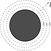
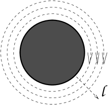
Figure 4.1: Left- and right-handed diffractive creeping paths of increasing mode number $\ell$ for a single disk.

We now turn to the semiclassical approximation of the coherent part of (3.9), namely the ratio of the determinants of the multiscattering matrix M. Because of the trace-class property of ${\bf A}={\bf M}-{\bf 1}$, the determinants in the numerator and denominator of this ratio exist individually and their semiclassical approximations can be studied separately. In fact, because of ${\rm Det}{\bf M}(k^{\ast})^{\dagger}=({\rm Det}{\bf M}(k^{\ast}))^{\ast}$, the semiclassical reduction of ${\rm Det}{\bf M}(k^{\ast})^{\dagger}$ follows directly from the corresponding result of ${\rm Det}{\bf M}(k)$ under complex conjugation. The semiclassical reduction of ${\rm Det}{\bf M}(k)$ will be done in the cumulant expansion, since the latter is the defining prescription for the computation of an infinite matrix that is of the form ${\bf 1}+{\bf A}$ where ${\bf A}$ is trace-class:

$${\rm Det}\left[{\bf 1}+z{\bf A}(k)\right] = 1-(-z){\rm Tr}[{\bf A}(k)]-\frac{z^{2}}{2}\left\{{\rm Tr}\left[{\bf A}^{2}(k)\right]-\left[{\rm Tr}{\bf A}(k)\right]^{2}\right\}+\cdots$$ (4.5)

$$= \sum_{n_{c}=0}^{\infty}z^{n_{c}}Q_{n_{c}}({\bf A})\qquad\mbox{with}\ Q_{0}({\bf A})\equiv 1$$

where we have introduced here a book-keeping variable $z$ which we will finally set to one. This allows us to express the determinant of the multiscattering matrix solely by the traces of the matrix ${\bf A}$, ${\rm Tr}[{\bf A}^{m}(k)]$ with $m=1,2,3,\cdots$. The cumulants and traces satisfy the (Plemelj-Smithies) recursion relations (A.22)

$$Q_{n_{c}}({\bf A})=\frac{1}{n_{c}}\sum_{m=1}^{n_{c}}(-1)^{m+1}Q_{n_{c}-m}({\bf A}){\rm Tr}\left[{\bf A}^{m}\right]\qquad\mbox{for}\ n_{c}\geq 1$$ (4.6)

in terms of the traces. In the next section we will utilize Watson resummation techniques [64, 29] which help to replace the angular momentum sums of the traces by continuous integrals which, in turn, allow for semiclassical saddle-point approximations. With these techniques and under complete induction we will show that for any geometry of $n$ disks, as long as the number of disks is finite, the disks do not overlap and grazing or penumbra situations [31, 35] are excluded (in order to guarantee unique isolated saddles), the semiclassical reduction reads as follows:

$${\rm Tr}\left[{\bf A}^{m}(k)\right]\ \stackrel{{\scriptstyle\rm s.c.}}{{\longrightarrow}}\ (-1)^{m}\sum_{p}\sum_{r>0}\delta_{m,rn_{p}}n_{p}\frac{{t_{p}(k)}^{r}}{1-\left(\frac{1}{\Lambda_{p}}\right)^{r}}+\mbox{creeping p.o.'s}\;$$ (4.7)

with inputs as defined below (2.3). The reduction is of course only valid, if ${\rm Re}\,k$ is sufficiently large compared to the inverse of the smallest length scale of the problem. The right hand side of Eq.(4.7) can be inserted into the recursion relation (4.6) which then reduces to a recursion relation for the semiclassical approximations of the quantum cumulants

$$C_{n_{c}}({\rm s.c.})=-\frac{1}{n_{c}}\sum_{m=1}^{n_{c}}C_{n_{c}-m}({\rm s.c.})\sum_{p}\sum_{r>0}\delta_{m,rn_{p}}n_{p}\frac{{t_{p}(k)}^{r}}{1-\left(\frac{1}{\Lambda_{p}}\right)^{r}}\quad\mbox{for}\ n_{c}\geq 1$$ (4.8)

where we have neglected the creeping orbits for the time being. Under the assumption that the semiclassical limit ${\rm Re}\,k\to\infty$ and the cumulant limit $n_{c}\to\infty$ commute (which might be problematic as we will discuss later), the approximate cumulants $C_{n_{c}}({\rm s.c.})$ can be summed to infinity, $\sum_{n_{c}=0}^{\infty}z^{n_{c}}C_{n_{c}}({\rm s.c.})$, in analogy to the exact cumulant sum. The latter exists since ${\bf A}$ is trace-class. The infinite “approximate cumulant sum”, however, is nothing but the curvature expansion of the Gutzwiller-Voros zeta function, i.e.,

$$Z_{\rm GV}(z;k)|_{\rm curv.\,reg.}=\sum_{n_{c}=0}^{\infty}z^{n_{c}}C_{n_{c}}({\rm s.c.})\;,$$ (4.9)

since Eq.(4.8) is exactly the recursion relation of the semiclassical curvature terms [2].

If, in addition, the creeping periodic orbits are summed as well, the standard Gutzwiller-Voros zeta function generalizes to the diffractive one discussed in Refs.[32, 33, 34] which we will denote here by a tilde. In summary, we have

$${\rm Det}{\bf M}(k)\ \stackrel{{\scriptstyle\rm s.c.}}{{\longrightarrow}}\ {\widetilde{Z}}_{\rm GV}(k)|_{\rm curv.\,reg.}$$ (4.10)

for a general geometry and

$${\rm det}{\bf M}_{{\rm D}_{c}}(k)\ \stackrel{{\scriptstyle\rm s.c.}}{{\longrightarrow}}\ {\widetilde{Z}}_{{\rm D}_{c}}(k)|_{\rm curv.\,reg.}$$ (4.11)

for the case that there is a finite point-symmetry and the determinant of the multiscattering matrix splits into the product of determinants of matrices belonging to the pertinent representations ${\rm D}_{c}$, see Eq.(3.12). Thus the semiclassical limit of the r.h.s. of Eq.(3.9) is

$${\rm det}_{{l}}{\bf S}^{(n)}(k) = \left\{\prod_{j=1}^{n}{\rm det}_{{l}}{\bf S}^{(1)}(ka_{j})\right\}\,\frac{{\rm Det}_{{L}}{{\bf M}(k^{\ast})}^{\dagger}}{{\rm Det}_{{L}}{\bf M}(k)}$$

$$\ \stackrel{{\scriptstyle\rm s.c.}}{{\longrightarrow}}\ \left\{\prod_{j=1}^{n}\left(\e^{-{\rm i}\pi N(ka_{j})}\right)^{2}\,\frac{{{\widetilde{Z}}_{{\rm 1\mbox{-}disk(l)}}(k^{\ast}a_{j})}^{\ast}}{{\widetilde{Z}}_{{\rm 1\mbox{-}disk(l)}}(ka_{j})}\,\,\frac{{{\widetilde{Z}}_{{\rm 1\mbox{-}disk(r)}}(k^{\ast}a_{j})}^{\ast}}{{\widetilde{Z}}_{{\rm 1\mbox{-}disk(r)}}(ka_{j})}\,\right\}\,\frac{{{\widetilde{Z}}_{\rm GV}(k^{\ast})}^{\ast}}{{\widetilde{Z}}_{\rm GV}(k)}\;,$$

where, from now on, we will suppress the qualifier $\cdots|_{\rm curv.\,reg.}$. For systems which allow for complete symmetry reductions (i.e., equivalent disks under a finite point-symmetry with $a_{j}=a\ \forall j$) the link reads

$${\rm det}_{{l}}{\bf S}^{(n)}(k) = \left({\rm det}_{{l}}{\bf S}^{(1)}(ka)\right)^{n}\frac{\prod_{c}\left({\rm det}_{{l_{c}}}{{\bf M}_{{\rm D}_{c}}(k^{\ast})}^{\dagger}\right)^{d_{c}}}{\prod_{c}\left({\rm det}_{{l_{c}}}{{\bf M}_{{\rm D}_{c}}(k)}\right)^{d_{c}}}$$ (4.13)

$$\ \stackrel{{\scriptstyle\rm s.c.}}{{\longrightarrow}}\ \left(\e^{-{\rm i}\pi N(ka)}\right)^{2n}\,\left(\frac{{{\widetilde{Z}}_{\rm 1\mbox{-}disk(l)}(k^{\ast}a)}^{\ast}}{{{\widetilde{Z}}_{\rm 1\mbox{-}disk(l)}(ka)}}\,\frac{{{\widetilde{Z}}_{\rm 1\mbox{-}disk(r)}(k^{\ast}a)}^{\ast}}{{{\widetilde{Z}}_{\rm 1\mbox{-}disk(r)}(ka)}}\right)^{n}\times$$

$$\qquad\qquad\qquad\times\frac{\prod_{c}\left({{\widetilde{Z}}_{{\rm D}_{c}}(k^{\ast})}^{\ast}\right)^{d_{c}}}{\prod_{c}\left({{\widetilde{Z}}_{{\rm D}_{c}}(k)}\right)^{d_{c}}}$$

in obvious correspondence. Note that the symmetry reduction from the right hand side of (LABEL:gen) to the right hand side of (4.13) is compatible with the semiclassical results of Refs.[65, 66].

In the next section we will prove the semiclassical reduction step (4.7) for any $n$-disk scattering system under the conditions that the number of disks is finite, the disks do not overlap, and geometries with grazing periodic orbits are excluded. We will also derive the general expression for creeping periodic orbits for $n$-disk repellers from exact quantum mechanics and show that ghost orbits drop out of the expansion of ${\rm Tr}\ln({\bf 1}+{\bf A})$ and therefore out of the cumulant expansion.

5 Semiclassical approximation and periodic orbits

In this section we will work out the semiclassical reduction of ${\rm Tr}[\,{\bf A}^{m}(k)\,]$ for non-overlapping, finite $n$-disk systems where

$${\bf A}^{jj^{\prime}}_{ll^{\prime}}=(1-\delta_{jj^{\prime}})\frac{a_{j}J_{l}(ka_{j})}{a_{j^{\prime}}H^{(1)}_{l^{\prime}}(ka_{j^{\prime\prime}})}(-1)^{l^{\prime}}\e^{{\rm i}(l\alpha_{j^{\prime}j}-l^{\prime}\alpha_{jj^{\prime}})}H^{(1)}_{l-l^{\prime}}(kR_{jj^{\prime}})\;.$$ (5.1)

As usual, $a_{j}$, $a_{j^{\prime}}$ are the radii of disk $j$ and $j^{\prime}$, $1\leq j,j^{\prime}\leq n$, $R_{jj^{\prime}}$ is the distance between the centers of these disks, and $\alpha_{j^{\prime}j}$ is the angle of the ray from the origin of disk $j$ to the one of disk $j^{\prime}$ as measured in the local coordinate system of disk $j$. The angular momentum quantum numbers $l$ and $l^{\prime}$ can be interpreted geometrically in terms of the positive– or negative-valued distances (impact parameters) $l/k$ and $l^{\prime}/k$ from the center of disk $j$ and disk $j^{\prime}$, respectively, see [49].

Because of the finite set of $n$ disk-labels and because of the cyclic nature of the trace, the object ${\rm Tr}[\,{\bf A}^{m}(k)\,]$ contains all periodic itineraries of total symbol length $m$ with an alphabet of $n$ symbols, i.e.  ${\bf A}^{j_{1}j_{2}}{\bf A}^{j_{2}j_{3}}\cdots{\bf A}^{j_{m-1}j_{m}}{\bf A}^{j_{m}j_{1}}$ with $j_{i}\in\{1,2,\dots,n\}$. Here the disk indices are not summed over and the angular momentum quantum numbers are suppressed for simplicity. The delta-function part $(1-\delta_{jj^{\prime}})$ generates the trivial pruning rule (valid for the full $n$-disk domain) that successive symbols have to be different. We will show that these periodic itineraries correspond in the semiclassical limit, $ka_{j_{i}}\gg 1$, to geometrical periodic orbits with the same symbolic dynamics. For periodic orbits with creeping sections [44, 45, 32, 33, 34] the symbolic alphabet has to be extended. Furthermore, depending on the geometry, there might be non-trivial pruning rules based on the so-called ghost orbits, see Refs.[7, 49]. We will discuss such cases in Sec.5.2.

5.1 Quantum itineraries

As mentioned, the quantum-mechanical trace can be structured by a simple symbolic dynamics, where the sole (trivial) pruning rule is automatically taken care of by the $1-\delta_{jj^{\prime}}$ factor appearing in ${\bf A}^{jj^{\prime}}_{ll^{\prime}}$. Thus we only have to consider the semiclassical approximation of a quantum-mechanical itinerary of length $m$:

$${\bf A}^{j_{1}j_{2}}{\bf A}^{j_{2}j_{3}}\cdots{\bf A}^{j_{m-1}j_{m}}{\bf A}^{j_{m}j_{1}}$$ (5.2)

$$:= \sum_{l_{1}=-\infty}^{+\infty}\sum_{l_{2}=-\infty}^{+\infty}\sum_{l_{3}=-\infty}^{+\infty}\cdots\sum_{l_{m-1}=-\infty}^{+\infty}\,\sum_{l_{m}=-\infty}^{+\infty}\,{\bf A}^{j_{1}j_{2}}_{l_{1}l_{2}}{\bf A}^{j_{2}j_{3}}_{l_{2}l_{3}}\cdots{\bf A}^{j_{m-1}j_{m}}_{l_{m-1}l_{m}}{\bf A}^{j_{m}j_{1}}_{l_{m}l_{1}}$$

with $j_{i}\in\{1,2,\dots,n\}$. This is still a trace in the angular momentum space, but not any longer with respect to the superspace. Since the trace, ${\rm Tr}{\bf A}^{m}$, itself is simply the sum of all itineraries of length $m$, i.e.

$${\rm Tr}{\bf A}^{m}=\sum_{j_{1}=1}^{n}\sum_{j_{2}=1}^{n}\sum_{j_{3}=1}^{n}\cdots\sum_{j_{m-1}=1}^{n}\sum_{j_{m}=1}^{n}\,{\bf A}^{j_{1}j_{2}}{\bf A}^{j_{2}j_{3}}\cdots{\bf A}^{j_{m-1}j_{m}}{\bf A}^{j_{m}j_{1}}\;,$$ (5.3)

its semiclassical approximation follows directly from the semiclassical approximation of its itineraries. Note that we here distinguish between a given itinerary and its cyclic permutation. All of them give the same result, such that their contributions can finally be summed up by an integer-valued factor $n_{p}:=m/r$, where the integer $r$ counts the number of repeated periodic subitineraries. Because of the pruning rule $1-\delta_{jj^{\prime}}$, we only have to consider traces and itineraries with $n\geq 2$ as ${\bf A}^{jj}_{ll^{\prime}}=0$ implies that ${\rm Tr}{\bf A}=0$ in the full domain.

We will show in this section that, with the help of the Watson method [64, 29] (studied for the convolution of two ${\bf A}$ matrices in App.F which should be consulted for details), the semiclassical approximation of the periodic itinerary

$${\bf A}^{j_{1}j_{2}}{\bf A}^{j_{2}j_{3}}\cdots{\bf A}^{j_{m-1}j_{m}}{\bf A}^{j_{m}j_{1}}$$

becomes a standard periodic orbit labelled by the symbol sequence $j_{1}j_{2}\cdots j_{m}$. Depending on the geometry, the individual legs $j_{i-1}\to j_{i}\to j_{i+1}$ result either from a standard specular reflection at disk $j_{i}$ or from a ghost path passing straight through disk $j_{i}$. If furthermore creeping contributions are taken into account, the symbolic dynamics has to be generalized from single-letter symbols $\{j_{i}\}$ to triple-letter symbols $\{j_{i},s_{i}\times\ell_{i}\}$ with $\ell_{i}\geq 1$ integer-valued and $s_{i}=0,\pm 1$  By definition, the value $s_{i}=0$ represents the non-creeping case, such that $\{j_{i},0\times\ell_{i}\}=\{j_{i},0\}=\{j_{i}\}$ reduces to the old single-letter symbol. The magnitude of a non-zero $\ell_{i}$ corresponds to creeping sections of mode number $|\ell_{i}|$, whereas the sign $s_{i}=\pm 1$ signals whether the creeping path turns around the disk $j_{i}$ in the positive or negative sense. Additional full creeping turns around a disk $j^{\prime}$ can be summed up as a geometrical series; therefore they do not lead to the introduction of a further symbol.

5.2 Ghost contributions

Figure 5.1: The ghost itinerary $(1,\underline{2},3,4)$.

An itinerary with a semiclassical ghost section at, say, disk $j_{i}$ will be shown to have the same weight as the corresponding itinerary without the $j_{i}$ th symbol. Thus, semiclassically, they cancel each other in the ${\rm Tr}\ln({\bf 1}+{\bf A})$ expansion, where they are multiplied by the permutation factor $m/r$ with the integer $r$ counting the repeats. E.g. let $(1,\underline{2},3,4)$ be a non-repeated periodic itinerary with a ghost section at disk 2 steming from the 4th-order trace ${\rm Tr}A^{4}$, where the convention is introduced that an underlined disk index signals a ghost passage (see Fig.5.1). Then its semiclassical, geometrical contribution to ${\rm Tr}\ln({\bf 1}+{\bf A})$ cancels exactly against the one of its “parent” itinerary $(1,3,4)$ (see Fig.5.2) resulting from the 3rd-order trace:

Figure 5.2: The parent itinerary $(1,3,4)$.

$$-\frac{1}{4}\left(4\,{\bf A}^{1,\underline{2}}_{\rm ghost}{\bf A}^{\underline{2},3}_{\rm ghost}{\bf A}^{3,4}_{\rm geom}{\bf A}^{4,1}_{\rm geom}\right)+\frac{1}{3}\left(3\,{\bf A}^{1,3}_{\rm geom}{\bf A}^{3,4}_{\rm geom}{\bf A}^{4,1}_{\rm geom}\right)$$

$$= (-1+1)\,{\bf A}^{1,3}_{\rm geom}{\bf A}^{3,4}_{\rm geom}{\bf A}^{4,1}_{\rm geom}=0\;.$$

The prefactors $+1/3$ and $-1/4$ are due to the expansion of the logarithm, the factors $3$ and $4$ inside the brackets result from the cyclic permutation of the periodic itineraries, and the cancellation stems from the rule

$$\cdots{\bf A}^{i,\underline{i+1}}_{\rm ghost}{\bf A}^{\underline{i+1},i+2}_{\rm ghost}\cdots=\cdots{\bf A}^{i,i+2}_{\rm geom}\cdots\;.$$ (5.5)

We have checked this rule in App.F.6 for the convolution of two ${\bf A}$-matrices, but in Sec.5.6 we will prove it to hold also inside an arbitrary (periodic) itinerary. Of course the same cancellation holds in case that there are two and more ghost segments. For instance, consider the itinerary $(1,\underline{2},3,4,\underline{5},6)$ with ghost sections at disk $2$ and $5$ resulting from the sixth order trace. Its geometrical contribution cancels in the trace-log expansion against the geometrical reduction of the itineraries $(1,\underline{2},3,4,,6)$, $(1,3,4,\underline{5},6)$ from the 5th-order trace with ghost sections at disk 2 or 5, respectively, and against the geometrical reduction of the itinerary $(1,3,4,6)$ of the 4th-order trace with no ghost contribution:

$$-\frac{1}{6}\left(6\,{\bf A}^{1,\underline{2}}_{\rm ghost}{\bf A}^{\underline{2},3}_{\rm ghost}{\bf A}^{3,4}_{\rm geom}{\bf A}^{4,\underline{5}}_{\rm ghost}{\bf A}^{\underline{5},6}_{\rm ghost}{\bf A}^{6,1}_{\rm geom}\right)$$

$$\mbox{}+\frac{1}{5}\left(5\,{\bf A}^{1,\underline{2}}_{\rm ghost}{\bf A}^{\underline{2},3}_{\rm ghost}{\bf A}^{3,4}_{\rm geom}{\bf A}^{4,6}_{\rm geom}{\bf A}^{6,1}_{\rm geom}+5\,{\bf A}^{1,3}_{\rm geom}{\bf A}^{3,4}_{\rm geom}{\bf A}^{4,\underline{5}}_{\rm ghost}{\bf A}^{\underline{5},6}_{\rm ghost}{\bf A}^{6,1}_{\rm geom}\right)$$

$$\mbox{}-\frac{1}{4}\left(4\,{\bf A}^{1,3}_{\rm geom}{\bf A}^{3,4}_{\rm geom}{\bf A}^{4,6}_{\rm geom}{\bf A}^{6,1}_{\rm geom}\right)$$

$$= (-1+2-1)\,{\bf A}^{1,3}_{\rm geom}{\bf A}^{3,4}_{\rm geom}{\bf A}^{4,6}_{\rm geom}{\bf A}^{6,1}_{\rm geom}=0\;.$$ (5.7)

Again, the prefactors $-1/4$, $+1/5$, $-1/6$ result from the trace-log expansion, the factors 4, 5, 6 inside the brackets are due to the cyclic permutations, and the rule (5.5) was used. If there are two or more ghost segments adjacent to each other, the ghost rule (5.5) has to be generalized to

$$\cdots{\bf A}^{i,\underline{i+1}}_{\rm ghost}{\bf A}^{\underline{i+1},\underline{i+2}}_{\rm ghost}\cdots{\bf A}^{\underline{i+k},\underline{i+k+1}}_{\rm ghosts}\cdots{\bf A}^{\underline{i+n-1},i+n}_{\rm ghosts}\cdots$$ (5.8)

$$= \cdots{\bf A}^{i,\underline{i+2}}_{\rm ghost}\cdots{\bf A}^{\underline{i+k},\underline{i+k+1}}_{\rm ghosts}\cdots{\bf A}^{\underline{i+n-1},i+n}_{\rm ghosts}\cdots$$

$$= {\cdots{\bf A}^{i,\underline{i+3}}_{\rm ghost}\cdots{\bf A}^{\underline{i+k},\underline{i+k+1}}_{\rm ghosts}\cdots{\bf A}^{\underline{i+n-1},i+n}_{\rm ghosts}\cdots}$$ (5.9)

$$= \cdots{\bf A}^{i,i+n}_{\rm geom}\cdots\;.$$ (5.10)

Finally, let us discuss one case with a repeat, e.g. the itinerary $(1,\underline{2},3,4,1,\underline{2},3,4)$ with repeated ghost sections at disk 2 in the semiclassical limit. The cancellations proceed in the trace-log expansion as follows:

$$-\frac{1}{8}\left(4\,{\bf A}^{1,\underline{2}}_{\rm ghost}{\bf A}^{\underline{2},3}_{\rm ghost}{\bf A}^{3,4}_{\rm geom}{\bf A}^{4,1}_{\rm geom}{\bf A}^{1,\underline{2}}_{\rm ghost}{\bf A}^{\underline{2},3}_{\rm ghost}{\bf A}^{3,4}_{\rm geom}{\bf A}^{4,1}_{\rm geom}\right)$$ (5.11)

$$\mbox{}+\frac{1}{7}\left(7\,{\bf A}^{1,\underline{2}}_{\rm ghost}{\bf A}^{\underline{2},3}_{\rm ghost}{\bf A}^{3,4}_{\rm geom}{\bf A}^{4,1}_{\rm geom}{\bf A}^{1,3}_{\rm geom}{\bf A}^{3,4}_{\rm geom}{\bf A}^{4,1}_{\rm geom}\right)$$

$$\mbox{}-\frac{1}{6}\left(3\,{\bf A}^{1,3}_{\rm geom}{\bf A}^{3,4}_{\rm geom}{\bf A}^{4,1}_{\rm geom}{\bf A}^{1,3}_{\rm geom}{\bf A}^{3,4}_{\rm geom}{\bf A}^{4,1}_{\rm geom}\right)$$

$$= \left(-\frac{1}{2}+1-\frac{1}{2}\right)\,\left[{\bf A}^{1,3}_{\rm geom}{\bf A}^{3,4}_{\rm geom}{\bf A}^{4,1}_{\rm geom}\right]^{2}=0$$

Note that the cyclic permutation factors of the 8th and 6th order trace are halved because of the repeat. The occurrence of the ghost segment in the second part of the 7th order itinerary is taken care of by the weight factor 7.

The reader might study more complicated examples and convince him- or herself that the rule (5.10) is sufficient to cancel any primary or repeated periodic orbit with one or more ghost sections completely out of the expansion of ${\rm Tr}\ln({\bf 1}+{\bf A})$ and therefore also out of the cumulant expansion in the semiclassical limit: Any periodic orbit of length $m$ with $n\mbox{($<m$)}$ ghost sections is cancelled by the sum of all ‘parent’ periodic orbits of length $m-i$ (with $1\leq i\leq n$ and $i$ ghost sections removed) weighted by their cyclic permutation factor and by the prefactor resulting from the trace-log expansion. This is the way in which the non-trivial pruning for the $n$-disk billiards can be derived from the exact quantum-mechanical expressions in the semiclassical limit. Note that there must exist at least one index $i$ in any given periodic itinerary which corresponds to a non-ghost section, since otherwise the itinerary in the semiclassical limit could only be straight and therefore non-periodic. Furthermore, the series in the ghost cancelation has to stop at the 2nd-order trace, ${\rm Tr}{\bf A}^{2}$, as ${\rm Tr}{\bf A}$ itself vanishes identically in the full domain which is considered here.

5.3 Semiclassical approximation of a periodic itinerary

The procedure for the semiclassical approximation of a general periodic itinerary, Eq.(5.2), of length $m$ follows exactly the calculation of App.F for the convolution of two ${\bf A}$-matrices. The reader interested in the details of the semiclassical reduction is advised to consult this appendix before proceeding with the remainder of the section. First, for any index $i$, $1\leq i\leq m$, the sum over the integer angular momenta, $l_{i}$, will be symmetrized as in Eq.(F.3) with the help of the weight function $d(l_{i})$ [$d(l_{i}\mbox{$\neq$}0)\equiv 1$, $d(l_{i}\mbox{=}0)=1/2$].

$${\bf A}^{j_{1}j_{2}}\cdots{\bf A}^{j_{i-1}j_{i}}{\bf A}^{j_{i}j_{i+1}}\cdots{\bf A}^{j_{m}j_{1}}$$

$$= \sum_{l_{1}=-\infty}^{+\infty}\sum_{l_{2}=-\infty}^{+\infty}\cdots\sum_{l_{i-1}=-\infty}^{+\infty}\sum_{l_{i}=-\infty}^{+\infty}\sum_{l_{i+1}=-\infty}^{+\infty}\cdots\sum_{l_{m}=-\infty}^{+\infty}{\bf A}^{j_{1}j_{2}}_{l_{1}l_{2}}\cdots{\bf A}^{j_{i-1}j_{i}}_{l_{i-1}l_{i}}{\bf A}^{j_{i}j_{i+1}}_{l_{i}l_{i+1}}\cdots{\bf A}^{j_{m}j_{1}}_{l_{m}l_{1}}$$

$$= \sum_{l_{1}=0}^{+\infty}\,\sum_{l_{2}=0}^{+\infty}\cdots\sum_{l_{i-1}=0}^{+\infty}\,\sum_{l_{i}=0}^{+\infty}\,\sum_{l_{i+1}=0}^{+\infty}\cdots\sum_{l_{m}=0}^{+\infty}\,\,\sum_{s_{1},\dots,s_{m}=-1,1}\,d(l_{1})\cdots d(l_{i-1})d(l_{i})\cdots d(l_{m})$$

$$\qquad\qquad\qquad\mbox{}\times{\bf A}^{j_{1}j_{2}}_{(s_{1}l_{1})(s_{2}l_{2})}\cdots{\bf A}^{j_{i-1}j_{i}}_{(s_{i-1}l_{i-1})(s_{i}l_{i})}{\bf A}^{j_{i}j_{i+1}}_{(s_{i}l_{i})(s_{i+1}l_{i+1})}\cdots{\bf A}^{j_{m}j_{1}}_{(s_{m}l_{m})(s_{1}l_{1})}\;.$$

Furthermore, the angles $\Delta\alpha_{j_{i}}\equiv\alpha_{j_{i+1}j_{i}}-\alpha_{j_{i-1}j_{i}}$ [the analogs of $\alpha_{j^{\prime\prime}j^{\prime}}-\alpha_{jj^{\prime}}$ in Eq.(F.3)] will be replaced by $\widetilde{\Delta}\alpha_{j_{i},\sigma_{i}}=\Delta\alpha_{j_{i}}-\sigma_{i}2\pi$ where $\sigma_{i}=0,2,1$. This will be balanced by multiplying Eq.(5.2) with $(-1)^{\sigma_{i}^{\prime}l_{i}}$ where $\sigma_{i}^{\prime}=\sigma_{i}$ for $\sigma_{i}=1$ and zero otherwise. The three choices for $\sigma_{i}$ are, at this stage, equivalent, but correspond in the semiclassical reduction to the three geometrical alternatives: specular reflection at disk $j_{i}$ to the right, to the left or ghost tunneling. In order not to be bothered by borderline cases between specular reflections and ghost tunneling, we exclude disk configurations which allow classically grazing or penumbra periodic orbits [31, 35].

Then, the sum over the integer angular momentum $l_{i}$ will be replaced by a Watson contour integration over the complex angular momentum $\nu_{i}$

$$\sum_{l_{i}=0}^{+\infty}\,(-1)^{l_{i}(1-\sigma^{\prime}_{i})}d(l_{i})X_{l_{i}}=\frac{1}{2{\rm i}}\oint_{C_{+}}{\rm d}{\nu_{i}}\,\frac{1}{\sin({\nu_{i}}\pi)}\e^{-{\rm i}\nu_{i}\pi\sigma_{i}^{\prime}}X_{\nu_{i}}\;,$$ (5.13)

as in Eq.(F.4). The quantity $X_{l_{i}}$ abbreviates here

$$X_{l_{i}}\! \equiv \frac{J_{l_{i}}(ka_{j_{i}})}{H^{(1)}_{l_{i}}(ka_{j_{i}})}\sum_{s_{i}=-1,1}\,H^{(1)}_{s_{i-1}l_{i-1}-s_{i}l_{i}}(kR_{j_{i-1}j_{i}})H^{(1)}_{s_{i}l_{i}-s_{i+1}l_{i+1}}(kR_{j_{i}j_{i+1}})\e^{{\rm i}s_{i}l_{i}\widetilde{\Delta}\alpha_{j_{i}\sigma_{i}}}$$ (5.14)

$$\equiv \frac{J_{l_{i}}(ka_{j_{i}})}{H^{(1)}_{l_{i}}(ka_{j_{i}})}Y_{l_{i}}$$

where the expression has simplified because of $J_{s_{i}l_{i}}(ka_{j_{i}})/H^{(1)}_{s_{i}l_{i}}(ka_{j_{i}})=J_{l_{i}}(ka_{j_{i}})/H^{(1)}_{l_{i}}(ka_{j_{i}})$, since $l_{i}$ is an integer. The quantity $Y_{l_{i}}$ abbreviates the sum in (5.14). The next steps are completely the same as in App.F.1–F.2. The paths below the real $\nu_{i}$ axis will be transformed above the axis. The expressions split into a $\sin(\nu_{i}\pi)$-dependent contour integral in the upper complex plane and into a $\sin(\nu_{i}\pi)$-independent straight-line integral from ${\rm i}\infty(1+{\rm i}\delta_{i})$ to $-{\rm i}\infty(1+{\rm i}\delta_{i})$. Depending on the choice of $\sigma_{i}$, the sum (5.13) becomes exactly one of the three expression (F.15), (F.16) or (F.17), where the prefactor $W^{jj^{\prime\prime}}_{ll^{\prime\prime}}$ in App.F.2 should be, of course, replaced by all the $l_{i}$-independent terms of Eq.(5.2) and where $j,j^{\prime},j^{\prime\prime}$ are substituted by by $j_{i-1},j_{i},j_{i+1}$. The angular momenta $l$ and $l^{\prime\prime}$ are here identified with $s_{i-1}\times l_{i-1}$ and $s_{i+1}\times l_{i+1}$, respectively. After the Watson resummation of the other sums, e.g., of the $l_{i-1}$ sum etc., $l$ has to be replaced by $\nu_{i-1}$ and $l^{\prime\prime}$ by $\nu_{i+1}$. If the penumbra scattering case [31, 35] is excluded, the choice of $\sigma_{i}$ is, in fact, uniquely determined from the empirical constraint that the creeping amplitude has to decrease during the creeping process, as tangential rays are constantly emitted. In mathematical terms, it means that the creeping angle has to be positive. As discussed at the beginning of App.F.2, the positivity of the two creeping angles for the left and right turn uniquely specifies which of the three alternatives $\sigma_{i}$ is realized. In other words, the geometry is encoded via the positivity of the two creeping paths into a unique choice of the $\sigma_{i}$. Hence, the existence of the saddle-point (5.15) is guaranteed.

The final step is the semiclassical approximation of the analog expressions to Eqs.(F.15)– (F.17) as in App.F.3–F.5. Whereas the results for the creeping contributions can be directly taken over from Eqs.(LABEL:res-alt-1) – (F.43), there is a subtle change in the semiclassical evaluation of the straight-line sections. In the convolution problem of App.F.3 and F.5 we have only picked up second-order fluctuating terms with respect to the saddle solution $\nu^{\prime}_{s}$ from the $\nu^{\prime}$ integration. Here, we will pick up quadratic terms $(\nu_{i}\mbox{$-$}\nu_{i}^{s})^{2}$ from the $\nu_{i}$ integration and mixed terms $(\nu_{i}\mbox{$-$}\nu_{i}^{s})(\nu_{i\pm 1}\mbox{$-$}\nu_{i\pm 1}^{s})$ from the neighboring $\nu_{i-1}$ and $\nu_{i+1}$ integrations as well. Thus instead of having $m$ one-dimensional decoupled Gauss integrations, we have one coupled $m$-dimensional one. Of course, also the saddle-point equations [the analog to Eq.(F.35) or (F.44)] are now coupled:

$$(1-\delta_{\sigma^{\prime}_{i},1})2\arccos[\nu_{i}^{s}/ka_{j_{i}}] = \arccos[(\nu_{i}^{s}-\nu_{i-1}^{s})/kR_{j_{i-1}j_{i}}]+\arccos[(\nu_{i}^{s}-\nu_{i+1}^{s})/kR_{j_{i}j_{i+1}}]$$ (5.15)

$$\mbox{}-(\alpha_{j_{i+1}j_{i}}-\alpha_{j_{i-1}j_{i}}-\sigma_{i}2\pi)$$

where the saddle $\nu_{i}^{s}$ of the $i$th integration depends on the values of the saddles of the $(i-1)$th and $(i+1)$th integration and so on. Indeed, all $m$ saddle-point equations are coupled. This corresponds to the fact that the starting- and end-point of a period orbit is not fixed from the outside, but has to be determined self-consistently, namely on the same footing as all the intermediate points.

In order to keep the resulting expressions simple we will discuss in the following subsection just the geometrical contributions, and leave the discussion of the ghost and creeping contributions for later sections.

5.4 Itineraries in the geometrical limit

We will prove that the itinerary $(-1)^{m}{\bf A}^{j_{1}j_{2}}{\bf A}^{j_{2}j_{3}}\cdots{\bf A}^{j_{m-1}j_{m}}{\bf A}^{j_{m}j_{1}}$ leads, in the semiclassical reduction, to the following geometrical contribution:

$$(-1)^{m}{\bf A}^{j_{1}j_{2}}{\bf A}^{j_{2}j_{3}}\cdots{\bf A}^{j_{m-1}j_{m}}{\bf A}^{j_{m}j_{1}}|_{\rm geom}=\frac{\e^{{\rm i}kL_{1\to m}-{\rm i}2m(\pi/2)}}{|\Lambda_{1\to m}|^{1/2}\left(1-\frac{1}{\Lambda_{1\to m}}\right)}\;,$$ (5.16)

where the factor $(-1)^{m}$ results from the trace-log expansion ${\rm Tr}ln({\bf 1}-[-{\bf A}])$, as the periodic orbit expansion corresponds to this choice of sign. The quantity $L_{1\to m}$ is the length of the periodic orbit with this itinerary. $\Lambda_{1\to m}>1$ is the expanding eigenvalue of the corresponding monodromy matrix and $\mu_{1\to m}=2m$ is the corresponding Maslov index indicating that the orbit is reflected from $m$ disks (all with Dirichlet boundary conditions). Thus, for $n$-disk Dirichlet problems, the Maslov indices come out automatically. [Under Neumann boundary conditions, there arises an additional minus sign per disk label $j_{i}$, since $\{\frac{d}{dk}H^{(2)}_{\nu_{i}}(ka_{j_{i}})\}/\{\frac{d}{dk}H^{(1)}_{\nu_{i}}(ka_{j_{i}})\}\simeq-H^{(2)}_{\nu_{i}}(ka_{j_{i}})/H^{(1)}_{\nu_{i}}(ka_{j_{i}})$ in the Debye approximation. The minus sign on the right-hand side cancels the original minus sign from the trace-log expansion such that the total Maslov index becomes trivial. Otherwise, the Neumann case is exactly the same.] If the itinerary is the $r$th repeat of a primary itinerary of topological length $p$, the length, Maslov index and stability eigenvalue will be shown to satisfy the relations: $L_{1\to m}=rL_{1\to p}$, $\mu_{1\to m}=r\mu_{1\to p}$ and $\Lambda_{1\to m}=(\Lambda_{1\to p})^{r}$.

Let us define the abbreviations

$$d_{i-1,i} \equiv \sqrt{R_{j_{i-1}j_{i}}^{2}-[(\nu_{i-1}^{s}-\nu_{i}^{s})/k]^{2}}=d_{i,i-1}$$ (5.17)

$$\rho_{i} \equiv \sqrt{a_{j_{i}}^{2}-(\nu_{i}^{s}/k)^{2}}$$ (5.18)

$$L_{i-1,i} \equiv d_{i-1,i}-\rho_{i-1}-\rho_{i}=L_{i,i-1}$$ (5.19)

$$\delta\nu_{i} \equiv \nu_{i}-\nu_{i}^{s}$$

$$\widetilde{\delta\nu}_{i} \equiv \frac{\delta\nu_{i}}{d_{i-1,i}^{1/2}}$$

with $i$ evaluated modulo $m$, especially $i=0$ is identified with $i=m$ and $i=m+1$ with $i=1$. The quantity $d_{i-1,i}$ is the geometrical length of the straight line between the impact parameter $\nu_{i-1}^{s}/k$ at disk $j_{i-1}$ and the impact parameter $\nu_{i}^{s}/k$ at disk $j_{i}$ in terms of the saddle points $\nu_{i-1}^{s}$ and $\nu_{i}^{s}$. The latter are determined by the saddle-point condition (5.15) which can be re-written for non-ghost scattering ($\sigma_{i}\neq 1$) as a condition on the reflection angle at disk $j_{i}$:

$$\theta_{j_{i}} \equiv \arcsin[\nu_{i}^{s}/ka_{j_{i}}]$$ (5.20)

$$= \arcsin\left[\frac{\nu_{i}^{s}\mbox{$-$}\nu_{i-1}^{s}}{kR_{j_{i-1}j_{i}}}\right]+\arcsin\left[\frac{\nu_{i}^{s}\mbox{$-$}\nu_{i+1}^{s}}{kR_{j_{i}j_{i+1}}}\right]+(\alpha_{j_{i+1}j_{i}}\mbox{$-$}\alpha_{j_{i-1}j_{i}}\mbox{$-$}\sigma_{i}2\pi)\;.$$

Thus, $\rho_{i}$ is the radius $a_{j_{i}}$ of the disk $j_{i}$ times the cosine of the reflection angle and $L_{i-1,i}$ is the geometrical length of the straight-line segment between the $(i\mbox{$-$}1)$th and $i$th point of reflection. Under the condition that the disks do not overlap, the inequalities $L_{i-1,i}<d_{i-1,i}<R_{j_{i-1}j_{i}}$ hold and exclude the possibility that the reflection points are in the mutual shadow region of disks. For each itinerary there is at most one reflection per disk-label $j_{i}$ modulo repeats, of course.

Then in analogy to App.F.5 the geometric limit of the itinerary (5.2) becomes

$$(-1)^{m}{\bf A}^{j_{1}j_{2}}{\bf A}^{j_{2}j_{3}}\cdots{\bf A}^{j_{m-1}j_{m}}{\bf A}^{j_{m}j_{1}}|_{\rm geom}$$ (5.21)

$$= (-1)^{m}\left\{\prod_{j=1}^{m}\int_{-\e^{-{\rm i}\pi/4}\infty}^{\e^{-{\rm i}\pi/4}\infty}{\rm d}\delta\nu_{j}\right\}\prod_{i=1}^{m}{\textstyle\frac{1}{2}}\e^{{\rm i}\pi/4}\sqrt{\frac{2}{\pi}}\frac{\e^{{\rm i}k(d_{i-1,i}-2\rho_{i})}}{k^{1/2}d_{i-1,i}^{1/2}}$$

$$\qquad\qquad\qquad\mbox{}\times\e^{-{\rm i}\frac{1}{2k}(\delta\nu_{i})^{2}\left(\frac{2}{\rho_{i}}-\frac{1}{d_{i-1,i}}-\frac{1}{d_{i,i+1}}\right)}\e^{-{\rm i}\frac{1}{2k}\delta\nu_{i}\delta\nu_{i+1}\frac{1}{d_{i,i+1}}}\e^{-{\rm i}\frac{1}{2k}\delta\nu_{i-1}\delta\nu_{i}\frac{1}{d_{i-1,i}}}$$

$$= \left\{\prod_{i=1}^{m}\frac{\e^{{\rm i}\pi/4}}{\sqrt{2\pi k}}\e^{{\rm i}k(d_{i-1,i}-2\rho_{i})-{\rm i}\pi}\right\}$$

$$\qquad\times\int_{-\e^{-{\rm i}\pi/4}\infty}^{\e^{-{\rm i}\pi/4}\infty}{\rm d}\widetilde{\delta\nu}_{1}\cdots\int_{-\e^{-{\rm i}\pi/4}\infty}^{\e^{-{\rm i}\pi/4}\infty}{\rm d}\widetilde{\delta\nu}_{m}\,\e^{-{\rm i}\frac{1}{2k}(\widetilde{\delta\nu}_{1}\cdots\widetilde{\delta\nu}_{m}){\bf F}_{1\to m}(\widetilde{\delta\nu}_{1}\cdots\widetilde{\delta\nu}_{m})^{T}}$$

$$= \frac{\e^{{\rm i}k\sum_{i=1}^{m}\,L_{i-1,i}-{\rm i}m\pi}}{|D_{1\to m}|^{1/2}}$$

where we have used that $\sum_{i=1}^{m}\,2\rho_{i}=\sum_{i}^{m}(\rho_{i-1}+\rho_{i})$ since $\rho_{0}=\rho_{m}$. $L_{1\to m}\equiv\sum_{i=1}^{m}L_{i-1,i}$ is the total geometrical length of the geometrical path around the itinerary, see App. G of Ref.[49]. Note that we used the saddle-point condition (5.15) in order to remove not only the linear fluctuations, but all terms of linear order in the $\nu_{i}^{s}$’s from the exponents. Only the zeroth-order terms and the quadratic fluctuations remain. $D_{1\to m}$ is the determinant of the $m\times m$ matrix ${\bf F}_{1\to m}$ ($\mbox{$\equiv$}{\bf F}$) with

$$\begin{array}[]{lclcl}{\bf F}_{1,1}&=&\frac{2d_{m,1}}{\rho_{1}}-1-\frac{d_{m,1}}{d_{1,2}}&\equiv&a_{1}\\ {\bf F}_{i,i}&=&\frac{2d_{i-1,i}}{\rho_{i}}-1-\frac{d_{i-1,i}}{d_{i,i+1}}&\equiv&a_{i}\quad{\rm for\ }2\leq i\leq m-1\\ {\bf F}_{m,m}&=&\frac{2d_{m-1,m}}{\rho_{m}}-1-\frac{d_{m-1,m}}{d_{m,1}}&\equiv&a_{m}\\ {\bf F}_{i,i+1}&=&\frac{d_{i-1,i}^{1/2}}{d_{i,i+1}^{1/2}}={\bf F}_{i+1,i}&\equiv&b_{i,i+1}\quad{\rm for}\ 1\leq i\leq m-1\\ {\bf F}_{m,1}&=&\frac{d_{m-1,m}^{1/2}}{d_{m,1}^{1/2}}={\bf F}_{1,m}&\equiv&b_{m,1}\\ {\bf F}_{i,j}&=&0\quad{\rm otherwise}&&\end{array}$$ (5.22)

for $m\geq 3$. [For $m=2$ the off-diagonal matrix elements read instead

$${\bf F}_{1,2}={\bf F}_{2,1}=\frac{d_{2,1}^{1/2}}{d_{1,2}^{1/2}}+\frac{d_{1,2}^{1/2}}{d_{2,1}^{1/2}}=2\;.$$ (5.23)

The corresponding diagonal matrix elements are given as above, but simplify because of $d_{2,1}=d_{1,2}$.] Thus in general, the determinant reads

$$D_{1\to m}={\rm det}\left(\begin{array}[]{ccccccc}a_{1}&b_{1,2}&0&0&\cdots&0&b_{m,1}\\ b_{1,2}&a_{2}&b_{2,3}&0&\cdots&0&0\\ 0&b_{2,3}&a_{3}&b_{3,4}&\ddots&\cdots&\vdots\\ 0&0&b_{3,4}&a_{4}&\ddots&\ddots&\vdots\\ \vdots&\cdots&\ddots&\ddots&\ddots&b_{m-2,m-1}&0\\ 0&0&\cdots&\ddots&\ddots&a_{m-1}&b_{m-1,m}\\ b_{m,1}&0&\cdots&\cdots&0&b_{m-1,m}&a_{m}\end{array}\right)\;.$$ (5.24)

Note that determinants of this structure can also be found in Balian and Bloch [7] and Berry [49]. Our task, however, is to simplify this expression, such that the stability structure of an isolated unstable periodic orbit emerges in the end. In order to derive a simpler expression for $D_{1\to m}$, let us consider the determinant $D_{1\to m}^{(0)}$ of the auxiliary $m\times m$ matrix ${\bf F}^{(0)}_{1\to m}$ ($\mbox{$\equiv$}{\bf F}^{(0)}$) which has the same matrix elements as ${\bf F}$ with the exception that $b_{m,1}=0$. The original determinant $D_{1\to m}$ can now be expressed as

$$D_{1\to m}=D_{1\to m}^{(0)}-\frac{d_{m-1,m}}{d_{m,1}}D_{2\to m-1}^{(0)}+2(-1)^{m+1}$$ (5.25)

where the last term follows from $\prod_{i=1}^{m}b_{i,i+1}=1$. Here and in the following $D_{l\to k}^{(0)}$ is defined as the determinant of the auxiliary $(k\mbox{$-$}l\mbox{+}1)\times(k\mbox{$-$}l\mbox{+}1)$ matrix ${\bf F}^{(0)}_{l\to k}$ with matrix elements ${\bf F}^{(0)}_{l\to k}|_{ij}={\bf F}_{ij}$ for $l\leq i,j\leq k(\leq m)$. Furthermore we define $D_{k+1\to k}^{(0)}\equiv{\bf F}_{k+1\to k}^{(0)}\equiv D_{1\to 0}^{(0)}\equiv 1$. The $D_{l\to k}^{(0)}$ determinants fulfill the following recursion relations

$$D_{l\to k}^{(0)} = \left(\frac{2d_{k-1,k}}{\rho_{k}}-1-\frac{d_{k-1,k}}{d_{k,k+1}}\right)D_{l\to k-1}^{(0)}-\frac{d_{k-2,k-1}}{d_{k-1,k}}D_{l\to k-2}^{(0)}\;,$$ (5.26)

$$D_{l\to k}^{(0)} = \left(\frac{2d_{l-1,l}}{\rho_{l}}-1-\frac{d_{l-1,l}}{d_{l,l+1}}\right)D_{l+1\to k}^{(0)}-\frac{d_{l-1,l}}{d_{l,l+1}}D_{l+2\to k}^{(0)}\;,$$ (5.27)

such that $D_{l\to k}^{(0)}$ can be constructed from all the lower determinants $D_{l\to j}^{(0)}$ and $D_{i\to j}^{(0)}$ with $l\leq i<j<k$. For example,

$$D_{1\to k}^{(0)} = -\frac{d_{k-1,k}}{d_{k,k+1}}D_{1\to k-1}^{(0)}+(-1)^{k}\left(1-\frac{2d_{m,1}}{\rho_{1}}D_{1\to 0}^{(0)}+\frac{2d_{1,2}}{\rho_{2}}D_{1\to 1}^{(0)}-\cdots\right.$$

$$\qquad\qquad\qquad\qquad\qquad\quad\mbox{}+\left.(-1)^{i}\frac{2d_{i-1,i}}{\rho_{i}}D_{1\to i-1}^{(0)}\cdots+(-1)^{k}\frac{2d_{k-1,k}}{\rho_{k}}D_{1\to k-1}^{(0)}\right)$$

and

$$D_{l\to k}^{(0)} = -\frac{d_{k-1,k}}{d_{k,k+1}}D_{l\to k-1}^{(0)}+(-1)^{k-l+1}\left(1-\frac{2d_{l-1,l}}{\rho_{l}}D_{l\to l-1}^{(0)}+\frac{2d_{l,l+1}}{\rho_{l+1}}D_{l\to l}^{(0)}\right.$$ (5.29)

$$\qquad\qquad\qquad\qquad\qquad\qquad\mbox{}+\left.\cdots+(-1)^{k-l+1}\frac{2d_{k-1,k}}{\rho_{k}}D_{l\to k-1}^{(0)}\right)$$

as can be shown by complete induction. Note that the product $d_{k,k+1}D_{l\to k}$ is a multinomial in $d_{j,j+1}/\rho_{i}$ where, for each index $j$, the $d_{j,j+1}/\rho_{i}$ factors appear at most once.

Replacing the $D_{1\to m}^{(0)}$ term in (5.25) by the r.h.s. of Eq.(LABEL:D0-recursion-full) and using the relation (5.27) in order to simplify the expression

$$-\frac{d_{m-1,m}}{d_{m,1}}(D_{1\to m-1}^{(0)}-D_{2\to m-1}^{(0)})$$

recursively, we finally find after some algebra that

$$D_{1\to m} = \frac{2d_{m-1,m}}{\rho_{m}}D_{1\to m-1}^{(0)}-\frac{2d_{m-2,m-1}}{\rho_{m-1}}D_{1\to m-2}^{(0)}+\cdots+(-1)^{i-1}\frac{2d_{m-i-1,m-i}}{\rho_{m-i}}D_{1\to m-i}^{(0)}$$ (5.30)

$$\mbox{}+\cdots+(-1)^{m-1}\frac{2d_{m,1}}{\rho_{1}}D_{1\to 0}^{(0)}$$

$$\!\!\!\!\!\!\!\!\mbox{}-\frac{2d_{m-1,m}}{\rho_{1}}D_{2\to m-1}^{(0)}+\frac{2d_{m-1,m}}{\rho_{2}}D_{3\to m-1}^{(0)}-\cdots+(-1)^{i-1}\frac{2d_{m-1,m}}{\rho_{i}}D_{i\to m-1}^{(0)}$$

$$\mbox{}+\cdots+(-1)^{m-1}\frac{2d_{m-1,m}}{\rho_{m-1}}D_{m\to m-1}^{(0)}\;.$$

By complete induction it can be shown that $D_{1\to m}$ is a multinomial in $2d_{i-1,i}/\rho_{j}$ of order $m$ where the single factors appear at most once and the highest term has the structure $\prod_{i=1}^{m}\,2d_{i-1,i}/\rho_{i}$. Thus, all the $d_{i-1,i}$’s are in the numerators, whereas all the $\rho_{i}$’s appear the denominators of this multinomial. We will show in Sec.5.9 that

$$D_{1\to m}=(-1)^{m}\left(\Lambda_{1\to m}+\frac{1}{\Lambda_{1\to m}}-2\right)$$ (5.31)

where $\Lambda_{1\to m}$ is the expanding eigenvalue of the monodromy matrix which belongs to that period orbit which is given by the geometric path of the periodic itinerary. If the result of Eq.(5.31) is inserted into Eq.(5.21) the semiclassical reduction (5.16) is proven.

5.5 Itineraries with repeats

In the following we will discuss modifications, if the periodic itinerary is repeated $r$ times, i.e., let $m=p\times r$ still be the total topological length of the itinerary, whereas $p$ is the length of the prime periodic unit which is repeated $r$ times:

$${\bf A}^{j_{1}j_{2}}\cdots{\bf A}^{j_{i-1}j_{i}}{\bf A}^{j_{i}j_{i+1}}\cdots{\bf A}^{j_{m}j_{1}}=\left[{\bf A}^{j_{1}j_{2}}\cdots{\bf A}^{j_{i-1}j_{i}}{\bf A}^{j_{i}j_{i+1}}\cdots{\bf A}^{j_{p}j_{1}}\right]^{r}\;.$$ (5.32)

The length and Maslov index of the itinerary are of course $r$ times the length and Maslov index of the primary itinerary ${\bf A}^{j_{1}j_{2}}\cdots{\bf A}^{j_{p}j_{1}}$, e.g., $L_{1\to m}=rL_{1\to p}$. The non-trivial point is the structure of the stability determinant $D_{1\to m}$. Here we can use that the matrix ${\bf F}_{1\to m}$ has exactly the structure of the matrices considered by Balian and Bloch in Ref.[7], Sec. 6 D. Let ${\bf F}_{1\to p}$ be the corresponding matrix of the primary itinerary with matrix elements as in Eqs.(5.22) [where $m$ is replaced by $p$ of course]. Following ref.[7] we furthermore define a new matrix $\widetilde{\bf F}_{p}(\chi)$ with matrix elements

$$\widetilde{\bf F}_{p}(\chi)|_{1,p} = \e^{-{\rm i}\chi}{\bf F}_{1\to p}|_{1,p}$$

$$\widetilde{\bf F}_{p}(\chi)|_{p,1} = \e^{{\rm i}\chi}{\bf F}_{1\to p}|_{p,1}$$

$$\widetilde{\bf F}_{p}(\chi)|_{i,j} = {\bf F}_{1\to p}|_{i,j}\quad{\rm otherwise}\;.$$

The determinant of the total itinerary is then [7]

$$D_{1\to m}=\prod_{n=1}^{r}\,\widetilde{D}_{1\to p}(\e^{{\rm i}2\pi n/r})\;$$ (5.33)

in terms of the $r$th roots of unity, since after $r$ repeats, the prefactor in front of the $(1,m)$ and $(m,1)$ matrix elements must be unity in order to agree with the original expression (5.22). Let us furthermore define

$$\alpha_{p} \equiv {\textstyle\frac{1}{2}}\left(\sqrt{\widetilde{D}_{1\to p}(0)}+\sqrt{\widetilde{D}_{1\to p}(\pi)}\right)$$

$$\beta_{p} \equiv {\textstyle\frac{1}{2}}\left(\sqrt{\widetilde{D}_{1\to p}(0)}-\sqrt{\widetilde{D}_{1\to p}(\pi)}\right)$$ (5.34)

then, according to Balian and Bloch [7], Sec. 6 D,

$$D_{1\to m} = (\alpha_{p}^{r}-(-\beta_{p})^{r})^{2}$$

$$= \alpha_{p}^{2r}+\beta_{p}^{2r}-2(-\alpha_{p}\beta_{p})^{r}\;.$$

In our case we have the further simplification (in analogy to Eq.(5.25))

$$-\alpha_{p}\beta_{p} = -\frac{1}{4}\left(\widetilde{D}_{1\to p}(0)-\widetilde{D}_{1\to p}(\pi)\right)$$

$$= -\frac{1}{4}\left(2(-1)^{p+1}-\{-2(-1)^{p+1}\}\right)=(-1)^{p}\;,$$

as the corresponding two matrices differ only in the sign of the their $(1,p)$ and $(p,1)$ elements. Especially we now have $\beta_{p}=(-1)^{p+1}/\alpha_{p}$, such that

$$D_{1\to m}=(\alpha_{p}^{2})^{r}+\frac{1}{(\alpha_{p}^{2})^{r}}-2(-1)^{pr}$$

which corresponds to the usual form

$$D_{1\to m}=(-1)^{pr}\left(\Lambda_{1\to p}^{r}+\frac{1}{\Lambda_{1\to p}^{r}}-2\right)$$ (5.35)

if $\Lambda_{1\to p}$ is identified with $(-1)^{p}\alpha_{p}^{2}$. Note that from this the structure of Eq.(5.31) follows for the special case $r=1$. Thus we have achieved so far two things: we have proven that the determinant $D_{1\to m}$ organizes itself in the same way as a monodromy matrix does and, in fact, that it can be written in terms of a monodromy matrix ${\bf M}_{1\to p}$ with eigenvalues $\Lambda_{1\to p}$, $1/\Lambda_{1\to p}$ as follows

$$D_{1\to m}=(-1)^{pr+1}{\rm det}({\bf M}_{1\to p}^{r}-{\bf 1})\;.$$ (5.36)

What is left to show is that ${\bf M}_{1\to p}$ is the very monodromy matrix belonging to the periodic orbit with the itinerary as in Eq.(5.32). This will be done in Sec.5.9. But first, we will complete the study of the geometrical sector by deriving the ghost subtraction rules, and furthermore discuss periodic orbits with creeping contributions.

5.6 Ghost rule

Let us now imagine that the itinerary (5.2) has, at the disk position $j_{i}$, an angular domain that corresponds to a ghost section, i.e. $\sigma_{i}=1$, $i$ fixed:

$${\bf A}^{j_{1}j_{2}}\cdots{\bf A}^{j_{i-1}\underline{j_{i}}}{\bf A}^{\underline{j_{i}}j_{i+1}}\cdots{\bf A}^{j_{m}j_{1}}\;.$$ (5.37)

Because of the cyclic nature of the itinerary we can always choose the label $j_{i}$ away from the first and end position [remember that at least two disk positions of any periodic orbit must be of non-ghost nature]. In this case there are four changes relative to the calculation in Eq.(5.21), see also App.F.6: first, the path of the $\nu_{i}$ integration is changed, second, there is a minus sign, third, the saddle-point condition at disk $j_{i}$ is given by Eq.(5.15) with $\sigma^{\prime}=1$ and not by (5.20), fourth, the $\rho_{i}$ terms are absent. As in App.F.6, the saddle condition (5.15) at the $j_{i}$th disk implies that $d_{i-1,i}+d_{i,i+1}=d_{i-1,i+1}$. We can use this in order to express the length of the ghost segment $L_{i-1,i+1}$ between the reflection point at disk $j_{i-1}$ and the next reflection point at disk $j_{i+1}$ in terms of the quantities defined in Eq.(5.19):

$$L_{i-1,i+1}=d_{i-1,i+1}-\rho_{i-1}-\rho_{i+1}=L_{i-1,i}+2\rho_{i}+L_{i,i+1}-\rho_{i-1}-\rho_{i+1}\;.$$ (5.38)

Thus, by adding and subtracting the $\rho_{i}$ contributions we get

$${\bf A}^{j_{1}j_{2}}\cdots{\bf A}^{j_{i-1}\underline{j_{i}}}{\bf A}^{\underline{j_{i}}j_{i+1}}\cdots{\bf A}^{j_{m}j_{1}}|_{\rm geom}$$ (5.39)

$$= \left\{\prod_{j=1,j\neq i}^{m}\,\int_{-\e^{-{\rm i}\pi/4}\infty}^{\e^{-{\rm i}\pi/4}\infty}{\rm d}\delta\nu_{j}\ \right\}\int_{\e^{+{\rm i}\pi/4}\infty}^{-\e^{+{\rm i}\pi/4}\infty}{\rm d}\delta\nu_{i}\,(-1)\e^{-{\rm i}\pi/2}\e^{{\rm i}k2\rho_{i}+{\rm i}\frac{1}{2k}(\delta\nu_{i})^{2}\frac{2}{\rho_{i}}}$$

$$\mbox{}\times\prod_{l=1}^{m}{\textstyle\frac{1}{2}}\e^{{\rm i}\pi/4}\sqrt{\frac{2}{\pi}}\frac{\e^{{\rm i}k(d_{l-1,l}-2\rho_{l})}}{k^{1/2}d_{l-1,l}^{1/2}}\e^{-{\rm i}\frac{1}{2k}(\delta\nu_{l})^{2}\left(\frac{2}{\rho_{l}}-\frac{1}{d_{l-1,l}}-\frac{1}{d_{l,l+1}}\right)}\e^{-{\rm i}\frac{1}{2k}\delta\nu_{l}\delta\nu_{l+1}\frac{1}{d_{l+1}}}\e^{-{\rm i}\frac{1}{2k}\delta\nu_{l-1}\delta\nu_{l}\frac{1}{d_{l}}}$$

$$= +\e^{{\rm i}k2\rho_{i}}\left\{\prod_{l=1}^{m}\frac{\e^{{\rm i}\pi/4}}{\sqrt{2\pi k}}\e^{{\rm i}k(d_{l-1,l}-2\rho_{l})}\right\}\prod_{j=1}^{m}\int_{-\e^{-{\rm i}\pi/4}\infty}^{\e^{-{\rm i}\pi/4}\infty}{\rm d}\widetilde{\delta\nu}_{j}\ \,\e^{-{\rm i}\frac{1}{2k}(\widetilde{\delta\nu}_{1}\cdots\widetilde{\delta\nu}_{m}){\bf F}_{1\to m}^{g_{i}}(\widetilde{\delta\nu}_{1}\cdots\widetilde{\delta\nu}_{m})^{T}}$$

$$= \frac{\e^{{\rm i}k\left(\sum_{l=1}^{m}L_{l-1,l}+2\rho_{i}\right)}}{|D^{g_{i}}_{1\to m}|^{1/2}}=\frac{\e^{{\rm i}k\left(\sum_{l=1}^{i-1}L_{l-1,l}+L_{i-1,i+1}+\sum_{l=i+2}^{m}L_{l-1,l}\right)}}{|D^{g_{i}}_{1\to m}|^{1/2}}\;.$$

[Note that the exponent of the ghost itinerary is exactly the same as of the one of its parent, the same itinerary without the disk $j_{i}$, whose geometrical path has the length $\sum_{l=1}^{i-1}L_{l-1,l}+L_{i-1,i+1}+\sum_{l=i+2}^{m}L_{l-1,l}$.] In writing down the last-but-one line we have cancelled the overall minus sign by exchanging the upper and lower limit of the $\delta\nu_{i}$ integration. In addition, the following substitutions were applied:

$$\begin{array}[]{lcl}\delta\nu_{l}&=:&d_{l-1,l}^{1/2}\,\widetilde{\delta\nu}_{l}\quad{\rm for}\ \ l\neq i,i+1\;,\\ \delta\nu_{i}&=:&\e^{{\rm i}\pi/2}\left(\frac{d_{i-1,i}d_{i,i+1}}{d_{i-1,i+1}}\right)^{1/2}\widetilde{\delta\nu}_{i}\;,\\ \delta\nu_{i+1}&=:&d_{i-1,i+1}^{1/2}\,\widetilde{\delta\nu}_{i+1}\;.\end{array}$$ (5.40)

In this way, the integration path and phase of the $i$th term agree with the ones of the other terms. $D^{g_{i}}_{1\to m}$ is the determinant of the $m\times m$ matrix ${\bf F}^{g_{i}}_{1\to m}$ ($\mbox{$\equiv$}{\bf F}^{g_{i}}$) which is affected by the substitutions in the following way:

$$\begin{array}[]{lcl}{\bf F}_{l,k}^{g_{i}}&=&{\bf F}_{l,k}\quad{\rm for}\ l,k\neq i,i+1\\ {\bf F}_{i,i}^{g_{i}}&=&1\\ {\bf F}_{i-1,i}^{g_{i}}&=&{\rm i}\left(\frac{d_{i-2,i-1}d_{i,i+1}}{d_{i-1,i}d_{i-1,i+1}}\right)^{1/2}={\bf F}_{i,i-1}^{g_{i}}\\ {\bf F}_{i,i+1}^{g_{i}}&=&{\rm i}\left(\frac{d_{i-1,i}}{d_{i,i+1}}\right)^{1/2}={\bf F}_{i+1,i}^{g_{i}}={\rm i}{\bf F}_{i,i+1}={\rm i}{\bf F}_{i+1,i}\\ {\bf F}_{i+1,i+1}^{g_{i}}&=&\frac{2d_{i-1,i+1}}{\rho_{i+1}}-\frac{d_{i-1,i+1}}{d_{i,i+1}}-\frac{d_{i-1,i+1}}{d_{i+1,i+2}}\\ {\bf F}_{i+1,i+2}^{g_{i}}&=&\left(\frac{d_{i-1,i+1}}{d_{i+1,i+2}}\right)^{1/2}={\bf F}_{i+2,i+1}^{g_{i}}\end{array}$$ (5.41)

where ${\bf F}_{l,k}$ are the matrix elements as defined Eqs.(5.22); i.e.,

$$D_{1\to m}^{g_{i}}={\rm det}\left({\bf F}^{g_{i}}\right)={\rm det}\left(\begin{array}[]{cccccc}\ddots&\ddots&\ddots&\vdots&\vdots&\cdots\\ \ddots&{\bf F}_{i-1,i-1}&{\bf F}_{i-1,i}^{g_{i}}&0&0&\cdots\\ \ddots&{\bf F}_{i,i-1}^{g_{i}}&1&{\bf F}_{i,i+1}^{g_{i}}&0&\cdots\\ \cdots&0&{\bf F}_{i+1,i}^{g_{i}}&{\bf F}_{i+1,i+1}^{g_{i}}&{\bf F}_{i+1,i+2}^{g_{i}}&\ddots\\ \cdots&0&0&{\bf F}_{i+2,i+1}^{g_{i}}&{\bf F}_{i+2,i+2}&\ddots\\ \vdots&\vdots&\vdots&\ddots&\ddots&\ddots\\ \end{array}\right)$$ (5.42)

We now subtract the $i$th row times ${\bf F}^{g_{i}}_{i,i-1}$ from the $(i\mbox{$-$}1)$th and the $i$th row times ${\bf F}_{i,i+1}^{g_{i}}$ form the $(i\mbox{+}1)$th, as both operations leave the determinant $D^{g_{i}}_{1\to m}$ unaffected. Using that the ghost segments add, i.e., $d_{i-1,i+1}=d_{i-1,i}+d_{i,i+1}$, the numerators of the terms in the $(i,i)$ and $(i\mbox{+}1,i\mbox{+}1)$ matrix elements can be simplified. The determinant $D_{1\to m}^{g_{i}}$, expressed via the transformed $m\times m$ matrix $\widetilde{\bf F}^{g_{i}}$, reads

$$D_{1\to m}^{g_{i}}={\rm det}\left(\widetilde{\bf F}^{g_{i}}\right)={\rm det}\left(\begin{array}[]{cccccc}\ddots&\ddots&\ddots&\vdots&\vdots&\cdots\\ \ddots&\widetilde{\bf F}_{i-1,i-1}&\widetilde{\bf F}_{i-1,i}^{g_{i}}&\widetilde{\bf F}_{i-1,i+1}^{g_{i}}&0&\cdots\\ \ddots&0&1&0&0&\cdots\\ \cdots&\widetilde{\bf F}_{i+1,i-1}^{g_{i}}&\widetilde{\bf F}_{i+1,i}^{g_{i}}&\widetilde{\bf F}_{i+1,i+1}^{g_{i}}&{\bf F}_{i+1,i+2}^{g_{i}}&\ddots\\ \cdots&0&0&{\bf F}_{i+2,i+1}^{g_{i}}&{\bf F}_{i+2,i+2}&\ddots\\ \vdots&\vdots&\vdots&\ddots&\ddots&\ddots\\ \end{array}\right)\;,$$ (5.43)

where

$$\begin{array}[]{lcl}\widetilde{\bf F}_{i-1,i-1}^{g_{i}}&=&\frac{2d_{i-2,i-1}}{\rho_{i-1}}-1-\frac{d_{i-2,i-1}}{d_{i-1,i+1}}\\ \widetilde{\bf F}_{i-1,i}^{g_{i}}&=&\cdots\\ \widetilde{\bf F}_{i-1,i+1}^{g_{i}}&=&\left(\frac{d_{i-2,i-1}}{d_{i-1,i+1}}\right)^{1,2}\\ \widetilde{\bf F}_{i+1,i-1}^{g_{i}}&=&\left(\frac{d_{i-2,i-1}}{d_{i-1,i+1}}\right)^{1,2}\\ \widetilde{\bf F}_{i+1,i}^{g_{i}}&=&\cdots\\ \widetilde{\bf F}_{i+1,i+1}^{g_{i}}&=&\frac{2d_{i-1,i+1}}{\rho_{i+1}}-1-\frac{d_{i-1,i+1}}{d_{i+1,i+2}}\;.\end{array}$$ (5.44)

Note that we do not have to specify the elements on the $i$th row explicitly, as the ones on the $i$th line satisfy $\widetilde{\bf F}^{g_{i}}_{i,l}=\delta_{i,l}$. For the same reason we can remove the $i$th line and row altogether without affecting the result for the determinant. In doing so, we exactly recover the determinant $D_{1\to i-1,i+2\to m}$ and matrix ${\bf F}_{1\to i-1,i+2\to m}$ of the parent itinerary of the considered “ghost”. [The parent itinerary has the same sequel of disk indices except that the disk $j_{i}$ is missing.]

$$D_{1\to m}^{g_{i}} = {\rm det}\left(\begin{array}[]{ccccc}\ddots&\ddots&\ddots&\vdots&\cdots\\ \ddots&{\bf F}_{i-1,i-1}&{\bf F}_{i-1,i+1}&0&\cdots\\ \cdots&{\bf F}_{i+1,i-1}&{\bf F}_{i+1,i+1}&{\bf F}_{i+1,i+2}&\ddots\\ \cdots&0&{\bf F}_{i+2,i+1}&{\bf F}_{i+2,i+2}&\ddots\\ \vdots&\vdots&\ddots&\ddots&\ddots\\ \end{array}\right)$$ (5.50)

$$= {\rm det}{\bf F}_{1\to i-1,i+2\to m}=D_{1\to i-1,i+2\to m}\;.$$ (5.51)

The contribution of the ghost segment itself to the total “stability” of the itinerary in the geometric limit, i.e. to the stability factor of the corresponding periodic orbit, is just trivially one. As also the geometrical lengths and signs of both itineraries are the same, we have finally found that

$${\bf A}^{j_{1}j_{2}}\cdots{\bf A}^{j_{i-1}\underline{j_{i}}}{\bf A}^{\underline{j_{i}}j_{i+1}}\cdots{\bf A}^{j_{m}j_{1}}|_{\rm geom}={\bf A}^{j_{1}j_{2}}\cdots{\bf A}^{j_{i-1}j_{i+1}}\cdots{\bf A}^{j_{m}j_{1}}|_{\rm geom}\;,$$ (5.52)

i.e., the ghost cancellation rule (5.5). Of course, the calculation of this section can trivially be extended to itineraries with more than one ghost (with and without repeats) as the operations in Eqs.(5.39), (5.40) and (5.43) are local operations involving just the segments with disk labels $j_{i}$, $j_{i-1}$ and $j_{i+1}$. Thus they can be performed successively without any interference. Furthermore, as the transformations of the pairs $(\delta\nu_{k},\delta\nu_{k+1})$ in (5.40) can be done iteratively (and in any order) for $k=i,i+1,\cdots$, the generalization to the extended ghost cancellation rule (5.10) is trivial as well:

$${{\bf A}^{j_{1}j_{2}}\cdots{\bf A}^{j_{i-1}\underline{j_{i}}}{\bf A}^{\underline{j_{i}}\underline{j_{i+1}}}{\bf A}^{\underline{j_{i+1}}{j_{i+2}}}\cdots{\bf A}^{j_{m}j_{1}}|_{\rm geom}}$$ (5.53)

$$= {{\bf A}^{j_{1}j_{2}}\cdots{\bf A}^{j_{i-1}\underline{j_{i}}}{\bf A}^{\underline{j_{i}}{j_{i+2}}}\cdots{\bf A}^{j_{m}j_{1}}|_{\rm geom}}$$

$$= {{\bf A}^{j_{1}j_{2}}\cdots{\bf A}^{j_{i-1}\underline{j_{i+1}}}{\bf A}^{\underline{j_{i+1}}{j_{i+2}}}\cdots{\bf A}^{j_{m}j_{1}}|_{\rm geom}}$$

$$= {{\bf A}^{j_{1}j_{2}}\cdots{\bf A}^{j_{i-1}{j_{i+2}}}\cdots{\bf A}^{j_{m}j_{1}}|_{\rm geom}}$$

etc.

5.7 Itineraries with creeping terms

Let us now study an itinerary of topological length $m$ which has, in the semiclassical limit, $m-1$ specular reflections and a left-handed or right-handed creeping contact with one disk (which we can put without lost of generality at the end position), i.e.

$${\bf A}^{j_{1}j_{2}}\cdots{\bf A}^{j_{m-2}j_{m-1}}{\bf A}^{j_{m-1}\widetilde{j_{m}}}{\bf A}^{\widetilde{j_{m}}j_{1}}|_{\rm sc+creep}\;.$$ (5.54)

We mark those disk positions with creeping contributions by a tilde. Using the results and methods of App.F.5 and Sec.5.3, we find the following result for the itinerary (5.54)

$${\bf A}^{j_{1}j_{2}}\cdots{\bf A}^{j_{m-2}j_{m-1}}{\bf A}^{j_{m-1}\widetilde{j_{m}}}{\bf A}^{\widetilde{j_{m}}j_{1}}|_{\rm sc+creep}$$ (5.55)

$$= -\sum_{\ell_{m}=1}^{\infty}\sum_{s_{m}=\pm 1}\frac{\e^{{\rm i}\pi/12}C_{\ell_{m}}}{(ka_{j_{m}})^{1/6}}\left(\frac{a_{j_{m}}}{\widetilde{d}_{m-1,s_{m}\ell_{m}}|\widetilde{D}^{(0)}_{1\to m-1}|}\right)^{1/2}\frac{\e^{{\rm i}\pi\widetilde{\nu}_{\ell_{m}}(1-\sigma_{m}^{\prime})}}{1-\e^{{\rm i}2\pi\widetilde{\nu}_{\ell_{m}}}}$$

$$\qquad\mbox{}\times\e^{{\rm i}s_{m}\widetilde{\nu}_{\ell_{m}}\left(\Delta\alpha_{j_{m}}-\pi\sigma_{m}+\arccos\left[\frac{\nu_{m-1}^{s}-s_{m}\widetilde{\nu}_{\ell_{m}}}{kR_{j_{m-1}j_{m}}}\right]-\arccos\left[\frac{s_{m}\widetilde{\nu}_{\ell_{m}}-\nu_{1}^{s}}{kR_{j_{m}j_{1}}}\right]\right)}$$

$$\qquad\mbox{}\times\e^{{\rm i}k[\widetilde{L}_{s_{m}\ell_{m},1}+\sum_{i=2}^{m-1}L_{i-1,i}+\widetilde{L}_{m-1,s_{m}\ell_{m}}]}\;.$$

Here, $\widetilde{\nu}_{\ell}\equiv\widetilde{\nu}_{\ell}(ka_{j_{m}})$ is the $\ell_{m}$th zero of the Hankel function $H^{(1)}_{\nu_{m}}(ka_{j_{m}})$ in the upper complex $\nu_{m}$ plane [and $C_{\ell_{m}}\equiv C_{\ell_{m}}(ka_{j_{m}})$ is the creeping coefficient as given by Eq.(F.33), see App.F.4], $\Delta\alpha_{j_{m}}$, $\sigma_{m}$ and $\sigma_{m}^{\prime}$ are defined in Sec.5.3, $d_{i-1,i}$, $\rho_{i}$ and $L_{i-1,i}$ are defined in Eqs.(5.17) – (5.19) and $\nu_{i}^{s}$ is the solution of the saddle-point equation (5.15) [where in the cases $i$=1 and $i$=$m\mbox{$-$}1$, the respective saddles $\nu_{i-1}^{s}$ and $\nu_{i+1}^{s}$ have to be replaced by $s_{m}\widetilde{\nu}_{\ell_{m}}$]. Furthermore, the following additional definitions have been introduced

$$\widetilde{d}_{m-1,s_{m}\ell_{m}} \equiv \left\{R_{j_{m-1}j_{m}}^{2}-\left(\frac{\nu_{m-1}^{s}-s_{m}\widetilde{\nu}_{\ell_{m}}}{k}\right)^{2}\right\}^{1/2}\equiv\widetilde{L}_{m-1,s_{m}\ell_{m}}+\rho_{m-1}$$ (5.56)

$$\widetilde{d}_{s_{m}\ell_{m},1} \equiv \left\{R_{j_{m}j_{1}}^{2}-\left(\frac{s_{m}\widetilde{\nu}_{\ell_{m}}-\nu_{1}^{s}}{k}\right)^{2}\right\}^{1/2}\equiv\widetilde{L}_{s_{m}\ell_{m},1}+\rho_{1}\;$$ (5.57)

which correspond to the geometrical lengths to the surface of disk $j_{m}$ if $\widetilde{\nu}_{\ell}$ is approximated by $ka_{j_{m}}$ (see below). Finally, $\widetilde{D}^{(0)}_{1\to m-1}$ is the determinant of the matrix $\widetilde{\bf F}^{(0)}_{1\to m-1}$ ($\mbox{$\equiv$}\widetilde{\bf F}^{(0)}$) with the matrix elements

$$\begin{array}[]{lclcl}\widetilde{\bf F}_{i,i}&=&\frac{2d_{i-1,i}}{\rho_{i}}-1-\frac{d_{i-1,i}}{d_{i,i+1}}&\equiv&a_{i}\quad{\rm for}\ 2\leq i\leq m-2\\ \widetilde{\bf F}_{1,1}&=&\frac{2\widetilde{d}_{s_{m}\ell_{m},1}}{\rho_{1}}-1-\frac{\widetilde{d}_{s_{m}\ell_{m},1}}{d_{1,2}}&\equiv&\widetilde{a}_{1}\\ \widetilde{\bf F}_{m-1,m-1}&=&\frac{2d_{m-2,m-1}}{\rho_{m-1}}-1-\frac{d_{m-2,m-1}}{d_{m-1,s_{m}\ell_{m}}}&\equiv&\widetilde{a}_{m-1}\\ \widetilde{\bf F}_{i,i+1}&=&\left(\frac{d_{i-1,i}}{d_{i,i+1}}\right)^{1/2}=\widetilde{\bf F}_{i+1,i}&\equiv&b_{i,i+1}\quad{\rm for}\ 2\leq i\leq m-2\\ {\bf F}_{1,2}&=&\left(\frac{\widetilde{d}_{s_{m}\ell_{m},1}}{d_{m,1}^{1/2}}\right)^{1/2}=\widetilde{\bf F}_{2,1}&\equiv&\widetilde{b}_{1,2}\\ \widetilde{\bf F}_{i,j}&=&0\quad{\rm otherwise}&&\end{array}\;.$$ (5.58)

Note that $\widetilde{D}^{(0)}_{1\to m-1}$ and $\widetilde{\bf F}^{(0)}_{1\to m-1}$ have exactly the form of the determinant $D^{(0)}_{1\to m-1}$ and the matrix ${\bf F}^{(0)}_{1\to m-1}$ defined in Sec.5.4 if the tilded lengths $\widetilde{d}_{s_{m}\ell,1}$ and $\widetilde{d}_{m-1,s_{m}\ell_{m}}$ are replaced by the “normal” geometrical lengths $d_{s_{m}m,1}$ and $d_{m-1,s_{m}m}$:

$$\widetilde{d}_{m-1,s_{m}\ell_{m}} \approx \left\{R_{j_{m-1}j_{m}}^{2}-(s_{m}a_{j_{m}}-\nu^{s}_{m-1}/k)^{2}\right\}\equiv d_{m-1,s_{m}m}$$ (5.59)

$$\widetilde{d}_{s_{m}\ell_{m},1} \approx \left\{R_{j_{m}j_{1}}^{2}-(s_{m}a_{j_{m}}-\nu^{s}_{1}/k)^{2}\right\}\equiv d_{s_{m}m,1}$$ (5.60)

As discussed in App.F.4, this approximation is justified in the leading Airy approximation, where terms of order $\hbar^{1/3}$ or higher are anyhow neglected. To this order we can approximate $\widetilde{\nu}_{\ell_{m}}$ everywhere by $ka_{j_{m}}$, except in the “creeping” exponential, since there the error would be of order $\hbar^{-1/3}$. Note that, in order to be consistent, we have to approximate $\widetilde{\nu}_{\ell_{m}}\approx ka_{j_{m}}$ in the saddle-point conditions for $\nu_{m-1}^{s}$ and $\nu_{1}^{s}$ as well. Thus, in this approximation, the saddles are manifestly real. Hence only in the overall factors in the exponents we keep the ${\cal O}(\hbar^{-1/3})$ term of

$$\widetilde{\nu}_{\ell_{m}} = ka_{j_{m}}+\e^{{\rm i}\frac{\pi}{3}}\left(\frac{ka_{j_{m}}}{6}\right)^{1\over 3}q_{\ell_{m}}$$ (5.61)

$$\equiv ka_{j_{m}}+\delta\widetilde{\nu}_{\ell_{m}}\;.$$

For all the other terms the errors from neglecting $\delta\widetilde{\nu}_{\ell_{m}}$ are, at least, of order ${\cal O}(\{\delta\widetilde{\nu}_{\ell_{m}}\}^{2}/k)={\cal O}(\hbar^{1/3})$ or even of ${\cal O}(\delta\widetilde{\nu}_{\ell_{m}}/k)={\cal O}(\hbar^{2/3})$. The expansion of the products $k\widetilde{d}_{m-1,s_{m}\ell_{m}}$ and $k\widetilde{d}_{s_{m}\ell_{m},1}$ in the exponents leads to potentially dangerous linear terms of order $\delta\widetilde{\nu}_{\ell_{m}}$. However, they cancel exactly against the terms in the expansion of the arccosines combined with those contributions which result if $\widetilde{\nu}_{\ell_{m}}\approx ka_{j_{m}}$ is inserted into the saddle-point relations for $\nu_{m-1}^{s}$ and $\nu_{1}^{s}$.

We will show below that in the leading Airy approximation, $\widetilde{d}_{m-1,s_{m}\l_{m}}\,|\widetilde{D}^{(0)}_{1\to m-1}|$ corresponds exactly to the effective radius of the creeping periodic orbit $R^{\rm eff}_{m\hookrightarrow m}$ defined in Ref.[32]. The latter quantity is constructed, as in Eq.(F.41), in terms of the length segments $l_{i-1,i}=L_{i-1,i}$ between the $(i\mbox{$-$}1)$th and $i$th point of reflection (if $2\leq i\leq m\mbox{$-$}1$), the length segments $l_{m,1}=d_{m,1}\mbox{$-$}\rho_{1}$ and $l_{m-1,m}=d_{m-1,m}\mbox{$-$}\rho_{m-1}$ between the (creeping) impact parameter at disk $j_{m}$ and the first or last point of reflection, respectively, and $\rho_{i}$ [= the radius $a_{j_{i}}$ of the disk $j_{i}$ times the cosine of the reflection angle]:

$$R^{\rm eff}_{m\hookrightarrow m} = l_{m,1}\prod_{i=1}^{m-1}\left(1+\kappa_{i}l_{i,i+1}\right)$$ (5.62)

$$= R^{\rm eff}_{m\hookrightarrow m-1}(1+\kappa_{m-1}l_{m-1,m})\;,$$

where the curvature $\kappa_{i}$ is given by the recursion relation

$$\kappa_{i}=\frac{1}{\kappa_{i-1}^{\ -1}+l_{i-1,i}}+\frac{2}{\rho_{i}}$$ (5.63)

with $1/\kappa_{0}\equiv 0$. The proof of the equivalence of $\widetilde{d}_{m-1,s_{m}\l_{m}}\,|\widetilde{D}^{(0)}_{1\to m-1}|$ and $R^{\rm eff}_{m\hookrightarrow m}$ uses the following relations, which can be derived from Eqs.(5.62) and (5.63) by complete induction:

$$R^{\rm eff}_{m\hookrightarrow j} = R^{\rm eff}_{m\hookrightarrow j-1}+\left(1+\frac{2R^{\rm eff}_{m\hookrightarrow 1}}{\rho_{1}}+\frac{2R^{\rm eff}_{m\hookrightarrow 2}}{\rho_{2}}+\cdots+\frac{2R^{\rm eff}_{m\hookrightarrow j-1}}{\rho_{j-1}}\right)l_{j-1,j}$$ (5.64)

$$\kappa_{j-1} = \frac{1}{R^{\rm eff}_{m\hookrightarrow j-1}}\left(1+\frac{2R^{\rm eff}_{m\hookrightarrow 1}}{\rho_{1}}+\frac{2R^{\rm eff}_{m\hookrightarrow 2}}{\rho_{2}}+\cdots+\frac{2R^{\rm eff}_{m\hookrightarrow j-1}}{\rho_{j-1}}\right)\;,$$ (5.65)

where $R^{\rm eff}_{m\hookrightarrow 0}\equiv 0$ and $R^{\rm eff}_{m\hookrightarrow 1}=l_{m,1}$. For the right hand side of the proof, the recursion relations (LABEL:D0-recursion-full) are applied to the combinations $|\widetilde{D}^{(0)}_{1\to j-1}|\widetilde{d}_{j-1,j}\approx D^{(0)}_{1\to j-1}d_{j-1,j}\equiv\widetilde{R}_{m\hookrightarrow j}$:

$$\widetilde{R}_{m\hookrightarrow j} = -\widetilde{R}_{m\hookrightarrow j-1}+(-1)^{j-1}\left(1-\frac{2\widetilde{R}_{m\hookrightarrow 1}}{\rho_{1}}+\frac{2\widetilde{R}_{m\hookrightarrow 2}}{\rho_{2}}-\cdots\right.$$ (5.66)

$$\qquad\qquad\qquad\qquad\qquad\left.\mbox{}+(-1)^{j-1}\frac{2\widetilde{R}_{m\hookrightarrow j-1}}{\rho_{j-1}}\right)d_{j-1,j}\;$$

with $\widetilde{R}_{m\hookrightarrow 0}\equiv 0$. In the induction assumption one can use that, for $1\leq j<m$. the quantities $\widetilde{R}_{m\hookrightarrow j}$ and $R^{\rm eff}_{m\hookrightarrow j}$ are related as

$$\widetilde{R}_{m\hookrightarrow j}=R^{\rm eff}_{m\hookrightarrow j}+\frac{R^{\rm eff}_{m\hookrightarrow j}-R^{\rm eff}_{m\hookrightarrow j-1}}{L_{j-1,j}}\,\rho_{j}\;.$$ (5.67)

This follows from the difference between $d_{j-1,j}$ and $l_{j-1,j}$. Note that $\widetilde{R}_{m\hookrightarrow 1}=d_{m,1}\mbox{=}L_{m,1}\mbox{+}\rho_{1}$ and $R^{\rm eff}_{m\hookrightarrow 1}=L_{m,1}$ satisfy trivially this induction ansatz. By complete induction it can now be shown that the recursion relation (5.66), applied to $\widetilde{R}_{m\hookrightarrow m}\equiv D^{(0)}_{1\to m-1}d_{m-1,m}$, can be rewritten as

$$\widetilde{R}_{m\hookrightarrow m} = R^{\rm eff}_{m\hookrightarrow m-1}+l_{m-1,m}\left\{1+\frac{2R^{\rm eff}_{m\hookrightarrow 1}}{\rho_{1}}+\cdots\frac{2R^{\rm eff}_{m\hookrightarrow i}}{\rho_{i}}+\cdots+\frac{2R^{\rm eff}_{m\hookrightarrow m-1}}{\rho_{m-1}}\right\}$$

$$\mbox{}+2l_{m-1,m}\left\{\frac{(-1)^{m-1}\mbox{$-$}1}{2}+\frac{(-1)^{m-2}\widetilde{R}_{m\hookrightarrow 1}\mbox{$-$}R^{\rm eff}_{m\hookrightarrow 1}}{\rho_{1}}+\cdots\right.$$

$$\qquad\qquad\quad\mbox{}\left.+\frac{(-1)^{m-i-1}\widetilde{R}_{m\hookrightarrow i}\mbox{$-$}R^{\rm eff}_{m\hookrightarrow i}}{\rho_{i}}+\cdots+\frac{\widetilde{R}_{m\hookrightarrow m-1}-R^{\rm eff}_{m\hookrightarrow m-1}}{\rho_{m-1}}\right\},$$

where the last bracket vanishes identically because of

$$\frac{\widetilde{R}_{m\hookrightarrow j}-R^{\rm eff}_{m\hookrightarrow j}}{\rho_{j}}=(1-\delta_{j,1})\,\frac{\widetilde{R}_{m\hookrightarrow j-1}-R^{\rm eff}_{m\hookrightarrow j-1}+2R^{\rm eff}_{m\hookrightarrow j-1}}{\rho_{j-1}}+\delta_{j,1}$$

for $1\leq j<m$. This equality can be derived from the induction ansatz Eq.(5.67), if Eq.(5.64) is inserted for the remaining $R^{\rm eff}_{m\hookrightarrow j}$ on the left hand side and for the remaining $R^{\rm eff}_{m\hookrightarrow j-1}$ on the right hand side. Thus, the equivalence $\widetilde{R}_{m\hookrightarrow m}\equiv D^{(0)}_{1\to m-1}\,d_{m-1,m}=R^{\rm eff}_{m\hookrightarrow m}$ is established in the leading Airy approximation.

We therefore get

$${\bf A}^{j_{1}j_{2}}\cdots{\bf A}^{j_{m-2}j_{m-1}}{\bf A}^{j_{m-1}\widetilde{j_{m}}}{\bf A}^{\widetilde{j_{m}}j_{1}}|_{\rm sc+creep}$$ (5.68)

$$\approx -\sum_{\ell_{m}=1}^{\infty}\sum_{s_{m}=\pm 1}\frac{\e^{{\rm i}\pi/12}C_{\ell_{m}}}{(ka_{j_{m}})^{1/6}}\left(\frac{a_{j_{m}}}{R^{\rm eff}_{m\hookrightarrow m}}\right)^{1/2}\e^{{\rm i}kL_{m\hookrightarrow m}(s_{m})}$$

$$\qquad\mbox{}\times\e^{{\rm i}(ka_{j_{m}}+\delta\widetilde{\nu}_{\ell_{m}})\left((2-\sigma_{m}^{\prime}-s_{m}\sigma_{m})\pi+s_{m}\Delta\alpha_{j_{m}}-\arccos\left[\frac{a_{j_{m}}{-}s_{m}{\nu_{m-1}^{s}}/{k}}{R_{j_{m-1}j_{m}}}\right]-\arccos\left[\frac{a_{j_{m}}{-}s_{m}{\nu_{1}^{s}}/{k}}{R_{j_{m}j_{1}}}\right]\right)}$$

$$\qquad\mbox{}\times\frac{1}{1-\e^{{\rm i}2\pi(ka_{j_{m}}+\delta\widetilde{\nu}_{\ell_{m}})}}\;,$$

where $L_{m\hookrightarrow m}\equiv L_{m,1}+\sum_{i=2}^{m-1}L_{i-1,i}+L_{m-1,m}$ is the total length of the straight geometrical sections. The impact parameter $\nu_{i}^{s}/k$ is given by the solution of the saddle-point equation (5.15) where, in the cases $i$=1 and $i$=$m\mbox{$-$}1$, the respective saddles $\nu_{i-1}^{s}/k$ and $\nu_{i+1}^{s}/k$, have to be replaced by $s_{m}a_{j_{m}}$.

In summary, all the quantities entering the semiclassical-creeping limit of the itinerary (5.68) with one creeping section have geometrical interpretations:

1. The integer index $\ell\geq 1$ enumerates the creeping modes around the boundary of disk $j_{m}$. With increasing $\ell$, the impact parameter (or distance of the creeping path from the surface of the disks) and the “tunneling” suppression factor increases.

2. The index $s_{m}=\pm 1$ distinguishes between creeping paths of positive sense or negative sense around a surface section of disk $j_{m}$.

3. The coefficient $\e^{{\rm i}\pi/12}C_{\ell_{m}}/(ka_{j_{m}})^{1/6}$ is proportional to the product of the two creeping diffraction constants at the beginning and end of the creeping segment along the boundary of disk $j_{m}$ which parameterize the transition from a straight section to a creeping section and vice versa, see [29, 30, 32].

4. The second prefactor is the inverse square root of the effective radius $R^{\rm eff}_{m\hookrightarrow m}$, in units of disk radius $a_{j_{m}}$. It is the geometrical amplitude, i.e., the geometrical stability factor.

5. The $\widetilde{\nu}_{\ell}$ independent terms in the exponents are just ${\rm i}k$ times the sum of all lengths of the straight geometrical segments of the periodic itinerary, i.e., $L_{m\hookrightarrow m}(s_{m})=L_{m,1}+\sum_{i=2}^{m-1}L_{i-1,i}+L_{m-1,m}$.

6. The geometrical length along the creeping section times ${\rm i}k$ is given by the sum of all exponential terms that are proportional to $a_{j_{m}}$.

7. The creeping “tunneling” suppression factor is given by the imaginary part of $\widetilde{\nu}_{\ell_{m}}$ or $\delta\widetilde{\nu}_{\ell_{m}}$.

8. The denominator $1-\e^{{\rm i}2\pi\widetilde{\nu}_{\ell_{m}}}$ results from the summation of all further complete creeping turns around the disk $j_{m}$, in terms of a geometrical series [32]. Note that the apparent poles at $1-\e^{{\rm i}2\pi\widetilde{\nu}_{\ell_{m}}}=0$ cancel against the corresponding semiclassical poles of one-disk S-matrix, ${\bf S}^{1}(ka_{j_{m}})$. In fact, the zeros of $1-\e^{{\rm i}2\pi\widetilde{\nu}_{\ell_{m}}}$ are given by $\widetilde{\nu}_{\ell_{m}}=l(\rm integer)$ and are nothing but the zeros of the Hankel function $H^{(1)}_{l}(ka_{j_{m}})$ in the Airy approximation.

5.8 More than one creeping section

The $r$th repeat of the itinerary (5.54) follows simply as the sum, $\sum_{\ell}\sum_{s_{m}}$, over the $r$th power of the summands on the r.h.s. of Eq.(5.55). As in the case of geometrical itineraries, this rule is trivial for the occurring prefactors, signs, phases and exponential terms. The non-trivial point is the behavior of the determinant $\widetilde{D}^{(0)}_{1\to m-1}$ under the $r$th repeat. However, as the corresponding matrix $\widetilde{\bf F}^{(0)}_{1\to m-1}$ has zero $(1,m\mbox{$-$}1)$ and $(m\mbox{$-$}1,1)$ matrix elements, such that repeats cannot couple here, the determinant of the $r$th repeat corresponds exactly to the $r$th power of the determinant of the primary itinerary. For the same reason, also the determinants and corresponding effective radii of itineraries, with more than one creeping contact (i.e., with at least two disks $j_{i}$ and $j_{m}$ with creeping contacts), decouple from each other. The corresponding semiclassical result for such an itinerary is thus the multiple sum, $\sum_{\ell_{i}}\sum_{s_{i}}\sum_{\ell_{m}}\sum_{s_{m}}$ over the products of the corresponding itinerary from disk $j_{i}$ to disk $j_{m}$ and the itinerary from disk $j_{m}$ to disk $j_{i}$, each individually given by the suitably adjusted summand on the r.h.s. of Eq.(5.55), e.g.:

$${\bf A}^{j_{1}j_{2}}\cdots{\bf A}^{j_{i-1}\widetilde{j_{i}}}{\bf A}^{\widetilde{j_{i}}j_{i+1}}\cdots{\bf A}^{j_{m-1}\widetilde{j_{m}}}{\bf A}^{\widetilde{j_{m}}j_{1}}|_{\rm sc+creep}$$

$$\approx \sum_{\ell_{i}=1}^{\infty}\sum_{s_{i}=\pm 1}\sum_{\ell_{m}=1}^{\infty}\sum_{s_{m}=\pm 1}$$

$$\qquad\mbox{}\times(-1)\frac{\e^{{\rm i}\pi/12}C_{\ell_{i}}}{(ka_{j_{i}})^{1/6}}\left(\frac{a_{j_{i}}}{R^{\rm eff}_{i\to m}}\right)^{1/2}\e^{{\rm i}kL_{i\to m}(s_{i},s_{m})}\,\frac{1}{1-\e^{{\rm i}2\pi(ka_{j_{i}}+\delta\widetilde{\nu}_{\ell_{i}})}}$$

$$\qquad\mbox{}\times\e^{{\rm i}(ka_{j_{i}}+\delta\widetilde{\nu}_{\ell_{i}})\left((2-\sigma_{i}^{\prime}-s_{i}\sigma_{i})\pi+s_{i}\Delta\alpha_{j_{i}}-\arccos\left[\frac{a_{j_{i}}-s_{i}\nu_{i-1}^{s}/k}{R_{j_{i-1}j_{i}}}\right]-\arccos\left[\frac{a_{j_{i}}-s_{i}\nu_{i+1}^{s}/k}{R_{j_{i}j_{i+1}}}\right]\right)}$$

$$\qquad\mbox{}\times(-1)\frac{\e^{{\rm i}\pi/12}C_{\ell_{m}}}{(ka_{j_{m}})^{1/6}}\left(\frac{a_{j_{m}}}{R^{\rm eff}_{m\hookrightarrow i}}\right)^{1/2}\e^{{\rm i}kL_{m\hookrightarrow i}(s_{m},s_{i})}\,\frac{1}{1-\e^{{\rm i}2\pi(ka_{j_{m}}+\delta\widetilde{\nu}_{\ell_{m}})}}$$

$$\qquad\mbox{}\times\e^{{\rm i}(ka_{j_{m}}+\delta\widetilde{\nu}_{\ell_{m}})\left((2-\sigma_{m}^{\prime}-s_{m}\sigma_{m})\pi+s_{m}\Delta\alpha_{j_{m}}-\arccos\left[\frac{a_{j_{m}}-s_{m}\nu_{m-1}^{s}/k}{R_{j_{m-1}j_{m}}}\right]-\arccos\left[\frac{a_{j_{m}}-s_{m}\nu_{1}^{s}/k}{R_{j_{m}j_{1}}}\right]\right)}\;,$$

etc. [If there are two (or more) creeping contacts next to each other, e.g., $j_{i}=j_{m-1}$, then, in the above formula, the corresponding impact parameters $\nu_{i+1}^{s}/k$ and $\nu_{m-1}^{s}/k$ have to be replaced by $a_{j_{m}}$ and $a_{j_{m-1}}$, respectively.]

The physical reason for the simple rule of piecing together creeping paths, is the point-like contact at e.g. disk $j_{i}$ between the creeping sections on the one hand and the geometrical sections on the other hand which is mediated by the diffraction constants $C_{\ell_{j}}$. [Mathematically, this corresponds to the fact that $\widetilde{\nu}_{\ell_{j}}$ is uniquely determined as the $\ell_{j}$th zero of the Airy integral and not by a semiclassical saddle-point equation that would couple with the saddle-point equations at the disks $j_{i-1}$ and $j_{i+1}$.] Because of this point-like contact [the independent determination of $\widetilde{\nu}_{\ell}$] the semiclassical itineraries multiply for fixed value of the mode numbers $\ell_{j}$ and creeping orientation $s_{j}$. Especially, if we limit the mode number to $\ell=1$, periodic orbits with common creeping sections can exactly be split up into their primary periodic orbits, see Ref.[32].

Finally, the ghost cancellation works for itineraries with creeping sections in the same way as for itineraries which, semiclassically, are purely geometrical. The reason is two-fold: First, by construction (see App.F.5), ghost segments can only occur in the geometrical part of the creeping itinerary. Second, the ghost cancellation rules of Sec.5.6 are based on the local properties of the segments $i\mbox{$-$}1\to i$ and $i\to i\mbox{+}1$. Let us now assume, for simplicity, that the disk $j_{i}$ is cut by the ghost section. If there is no creeping at the neighboring disks $j_{i-1}$ and $j_{i+1}$, the reduction of the stability matrix $\widetilde{\bf F}^{(0)}$ and of the phases and lengths of the segments is precisely the same as in the purely geometrical case (see the substitutions (5.40) and the analogous steps of Sec.5.6). If there is a creeping contact at disk $j_{i-1}$ or/and disk $j_{i+1}$, the substitutions (5.40) simplify, as $\delta\nu_{i-1}$ or/and $\delta\nu_{i+1}$ do not exist. Thus, the elements ${\bf F}_{i-1,i}^{g_{i}}$ or/and ${\bf F}_{i+1,i+1}^{g_{i}}$ of Eq.(5.41) are zero and the $i$th row of the determinant (5.42) has only to be subtracted from the $(i+1)$th or the $(i-1)$th row or from none, in order that Eq.(5.42) becomes Eq.(5.43). The reduction in the lengths and phases hold in these cases as before.

In summary, the ghost cancellation works for geometrical orbits with creeping sections as well as for purely geometrical orbits, studied in Sec.5.6. Semiclassically, neither the ghost itineraries nor their parent itineraries [which have the same symbol sequence except that the ghost labels are removed subsequently] contribute to the semiclassical trace-log expansion and to the cumulant/curvature expansion. Thus, one can omit these “ghost-affected” periodic orbits altogether from the curvature expansion.

Deep inside the negative complex $k$-plane the limitations of the first Airy correction introduce rather big errors, see Ref.[67]. In this case it is advisable to use to the original expression (5.55) for semiclassical “creeping” itineraries with $\widetilde{\nu}_{\ell_{m}}$ and $C_{\ell_{m}}$, as given in Eqs.(F.28) and (F.33), instead of Eq.(5.68).

To summarize, for the special case of $n$-disk repellers, the creeping periodic orbits of Ref.[32] have been recovered directly from quantum mechanics, whereas the construction of Ref.[32] has relied on Keller’s semiclassical theory of diffraction [30]. Furthermore, the symbol dynamics has to be generalized from the single-letter labelling $\{j_{i}\}$ to the two-letter labelling $\{j_{i},s_{i}\times\ell_{i}\}$ with $s_{i}=0,\pm 1$ and $\ell_{i}=1,2,3,\cdots$.

5.9 Geometrical stabilities

In this subsection we will return to purely geometrical periodic orbits and show that Eqs.(5.35) and (5.36) are correct, i.e. that the determinant $D_{1\to m}$ satisfies in fact

$$D_{1\to m} = (-1)^{m+1}{\rm det}({\bf M}_{1\to m}-{\bf 1})$$ (5.69)

$$= (-1)^{m}\left(\Lambda_{1\to m}+\frac{1}{\Lambda_{1\to m}}-2\right)\;$$

irrespective, whether there are repeats or not. Here ${\bf M}_{1\to m}$ is the 2$\times$2 dimensional real monodromy matrix of the purely geometrical periodic orbit of total topological length $m$ ($m=pr$ if there are $r$ repeats of a primary orbit of topological length $p$), that is, the semiclassical limit of the itinerary $A^{j_{m}j_{1}}\cdots A^{j_{m}j_{1}}$. Because of phase-space conservation, the determinant of ${\bf M}_{1\to m}$ is unity. For this reason and as the matrix elements of ${\bf M}_{1\to m}$ are real (see below), the two eigenvalues of the matrix are related as $\Lambda_{1\to m}$ and $1/\Lambda_{1\to m}$. We do not have to treat repeated orbits explicitly here, as this case was already studied in Sec.5.5.

In Ref.[15] it was shown that, for any two-dimensional scalar billiard problem (whether a bound state problem or a scattering problem), the monodromy matrix ${\bf M}_{1\to m}$ of a periodic orbit with $m$ collisions with the billiard walls is given by the 2$\times$2 dimensional Jacobian belonging to the infinitesimal evolution of the vector $(\delta p_{\perp},\delta x_{\perp})^{T}$ perpendicular to this classical trajectory in phase space, i.e., by the product

$${\bf M}_{1\to m}=\prod_{i=1}^{m}{\bf T}_{i-1,i}{\bf R}_{i}\;.$$ (5.70)

Here the matrix

$${\bf T}_{i-1,i}=\left(\begin{array}[]{c c}1&0\\ L_{i-1,i}&1\end{array}\right)$$ (5.71)

parametrizes the translational (straight ray) evolution of the vector $(\delta p_{\perp},\delta x_{\perp})^{T}$ [or rather $(\delta\theta_{p},\delta x_{\perp})^{T}$ with $\theta_{p}$ being the angle of the momentum $p$, since the modulus of $p$ is conserved anyhow] between the $(i\mbox{$-$}1)$th and $i$th collision where $L_{i-1,i}$ is the corresponding length segment. As usual $i\mbox{=}0$ should be identified with $i\mbox{=}m$. The matrix

$${\bf R}_{i}=\left(\begin{array}[]{c c}-1&-2/\rho_{i}\\ 0&-1\end{array}\right)$$ (5.72)

parametrizes the evolution of the vector $(\delta\theta_{p},\delta x_{\perp})^{T}$ from immediately before to immediately after the $i$th collision. The quantity $\rho_{i}\mbox{=}a_{i}\cos\theta_{i}$ is, in general, the product of the local radius of curvature $a_{i}$ and the cosine of the reflection angle $\theta_{i}$ at the $i$th collision with the billiard walls. Especially for our $n$-disk scattering problems, $a_{i}$ is of course nothing but $a_{j_{i}}$, the radius of the disk $j_{i}$, whereas $\theta_{i}$ should be identified with the scattering angle $\theta_{j_{i}}$ of Eq.(5.20), the solution of the saddle-point equation. Since the determinants ${\rm det}{\bf T}_{i-1,i}$ and ${\rm det}{\bf R}_{i}$ are trivially unity, the determinant of the product ${\bf M}_{1\to m}$ is unity as well, as it should because of Liouville’s theorem. Furthermore, the matrix elements of ${\bf M}_{1\to m}$ have to be real, since the matrices ${\rm det}{\bf T}_{i-1,i}$ and ${\rm det}{\bf R}_{i}$ are real, by definition. Thus the two eigenvalues of ${\bf M}_{1\to m}$ have the structure $\Lambda_{1\to m}$ and $1/\Lambda_{1\to m}$.

5.9.1 Monodromy matrix in closed form

In the following we will construct a closed-form expression for the matrix elements of the matrix ${\bf M}_{1\to n}$, $1\leq n$, by complete induction. Let us denote these matrix elements as

$${\bf M}_{1\to n}\equiv(-1)^{n}\left(\begin{array}[]{cc}A_{n}&B_{n}\\ C_{n}&D_{n}\end{array}\right)\;.$$ (5.73)

By inserting Eqs. (5.71) and (5.72) into Eq.(5.70), one can show that

$$\begin{array}[]{lcl}A_{1}&=&1\\ B_{1}&=&\frac{2}{\rho_{1}}\\ C_{1}&=&L_{0,1}\\ D_{1}&=&1+\frac{2L_{0,1}}{\rho_{1}}\end{array}$$ (5.74)

and that the matrix elements of ${\bf M}_{1\to n+1}$ and ${\bf M}_{1\to n}$ are related as follows:

$$A_{n+1} = A_{n}+B_{n}L_{n,n+1}$$ (5.75)

$$B_{n+1} = B_{n}\left(1+\frac{2L_{n,n+1}}{\rho_{n+1}}\right)+A_{n}\frac{2}{\rho_{n+1}}$$ (5.76)

$$C_{n+1} = C_{n}+D_{n}L_{n,n+1}$$ (5.77)

$$D_{n+1} = D_{n}\left(1+\frac{2L_{n,n+1}}{\rho_{n+1}}\right)+C_{n}\frac{2}{\rho_{n+1}}\;.$$ (5.78)

In order to be able to perform the induction step, we do not make use of the cyclic permutation, i.e., in the following we do not replace $L_{0,1}$ with $L_{n,1}$ or $L_{n+1,1}$, respectively, and $L_{n,n+1}$ or $L_{n+1,n+2}$ with $L_{n,1}$, but keep the original labelling. From Eqs.(5.74) and (5.78) it follows, by complete induction, that

$$A_{n} = 1+\sum_{i=1}^{n-1}\frac{2R^{\rm eff}_{i\to n}}{\rho_{i}}$$ (5.79)

$$B_{n} = \sum_{i=1}^{n}\left(1+\sum_{j=i+1}^{n}\frac{2R^{\rm eff}_{i\to j}}{\rho_{j}}\right)\frac{2}{\rho_{i}}=\sum_{i=1}^{n}\frac{R^{\rm eff}_{i\to n+1}-R^{\rm eff}_{i\to n}}{L_{n,n+1}}\,\frac{2}{\rho_{i}}$$ (5.80)

$$C_{n} = R^{\rm eff}_{0\to n}$$ (5.81)

$$D_{n} = 1+\sum_{i=1}^{n}\frac{2R^{\rm eff}_{0\to i}}{\rho_{i}}$$ (5.82)

with $R^{\rm eff}_{j\to n}$ given as in Eq.(5.62) where we identify $l_{i-1,i}$ with $L_{j+i-1,j+i}$. In analogy to Eq.(5.64), we can derive the recursion relation

$$R^{\rm eff}_{j\to n} = R^{\rm eff}_{j\to n-1}+\left(1+\sum_{i=1}^{n-1-j}R^{\rm eff}_{j\to j+i}\frac{2}{\rho_{j+i}}\right)L_{n-1,n}\;,$$ (5.83)

where $R^{\rm eff}_{j\to n}|_{j\geq n}\equiv 0$. Thus $R^{\rm eff}_{n\to n}$ should not be mixed up with the quantity $R^{\rm eff}_{n\hookrightarrow n}$ of Sec.5.7 that rather corresponds here to $R^{\rm eff}_{0\to n}$ with $l_{0,1}\equiv L_{0,1}$, of course. Note that the first iteration of Eq.(5.83) leads to $R^{\rm eff}_{j\to j+1}\equiv L_{j,j+1}$. For later purposes we also define here the effective radius $R^{\rm eff}_{j\leftarrow n}$ which is, of course, equal to $R^{\rm eff}_{j\to n}$ and which satisfies the recursion relation

$$R^{\rm eff}_{j\leftarrow n} = R^{\rm eff}_{j+1\leftarrow n}+L_{j,j+1}\left(1+\sum_{i=1}^{n-1-j}\frac{2}{\rho_{n-i}}R^{\rm eff}_{n-i\leftarrow n}\right)\;,$$ (5.84)

where again $R^{\rm eff}_{j\leftarrow n}|_{j\geq n}\equiv 0$, such that $R^{\rm eff}_{n-1\leftarrow n}=L_{n-1,n}$.

The second equation of Eq.(5.80) follows trivially from (5.83). By inserting the Ansätze (5.81) and (5.82) into the induction step (5.77), one can easily show, with the help of the recursion relation (5.83) (for the case $j=0$), that the result for $C_{n+1}$ is given by Eq.(5.81), with $n$ replaced by $n+1$. Similarly, by inserting the Ansätze (5.79) and the last identity of (5.80) into the induction step (5.75), one finds that $A_{n+1}$ is compatible with (5.79). Here we used the identity $R^{\rm eff}_{n\to n}\equiv 0$. Applying the recursion relation (5.83) to $R^{\rm eff}_{0\to n+1}$, it easy to show that $D_{n+1}$ is compatible with Eq.(5.81) as well. Finally, for proving that $B_{n+1}$ is compatible with Eq.(5.80), one inserts the first equation of (5.80) and (5.79) into (5.76), uses Eq.(5.83) for re-expressing $R^{\rm eff}_{i\to n+1}$ and the fact that $L_{n,n+1}=R^{\rm eff}_{n\to n+1}$.

Having a closed form expression for the matrix elements of ${\bf M}_{1\to m}$ we could now construct the corresponding eigenvalues $\Lambda_{1\to m}^{\pm 1}$. But, in fact, we only need the linear combination $(-1)^{m}(\Lambda_{1\to m}+1/\Lambda_{1\to m})$ which is equal to the sum $A_{m}+D_{m}$.

In summary, we have now a closed form expression for the right hand sides of Eq.(5.69)

$$(-1)^{m+1}{\rm det}({\bf M}_{1\to m}-{\bf 1}) = (-1)^{m}\left(\Lambda_{1\to m}+\frac{1}{\Lambda_{1\to m}}-2\right)$$ (5.85)

$$= 2(1+(-1)^{m+1})+\sum_{i=1}^{m}R^{\rm eff}_{0\to i}\frac{2}{\rho_{i}}+\sum_{i=1}^{m-1}\frac{2}{\rho_{i}}R^{\rm eff}_{i\leftarrow m}\;,$$

where we used the identity $R^{\rm eff}_{i\to m}=R^{\rm eff}_{i\leftarrow m}$ in writing down the last relation.

5.9.2 Stability determinant in closed form

In analogy to the definitions of Sec.5.7 [see Eq.(5.66)] we define here $D^{(0)}_{l+1\to k-1}d_{k-1,k}\equiv{\overline{R}}_{l\to k}\equiv{\overline{R}}_{l\leftarrow k}$. These quantities satisfy, according to Eq.(5.26), the recursion relations

$${\overline{R}}_{l\to k}+{\overline{R}}_{l\to k-1} = \left({\overline{R}}_{l\to k-1}\frac{2}{\rho_{k-1}}-\left[{\overline{R}}_{l\to k-1}+{\overline{R}}_{l\to k-2}\right]\frac{1}{d_{k-2,k-1}}\right)d_{k-1,k}$$ (5.86)

and, according to Eq.(5.27), the recursion relations

$${\overline{R}}_{l\leftarrow k}+{\overline{R}}_{l+1\leftarrow k} = d_{l,l+1}\left(\frac{2}{\rho_{l+1}}{\overline{R}}_{l+1\leftarrow k}-\frac{1}{d_{l+1,l+2}}\left[{\overline{R}}_{l+1\leftarrow k}+{\overline{R}}_{l+2\leftarrow k}\right]\right)\;.$$ (5.87)

By complete induction, these recursion relations can be summed up to give

$${\overline{R}}_{l\to k} = -{\overline{R}}_{l\to k-1}+(-1)^{k-l-1}\left(1+\sum_{i=1}^{k-l-1}(-1)^{i}\,\frac{2{\overline{R}}_{l\to l+i}}{\rho_{l+i}}\right)d_{k-1,k}$$ (5.88)

$$={\overline{R}}_{l\leftarrow k} = -{\overline{R}}_{l+1\leftarrow k}+(-1)^{k-l-1}\,d_{l,l+1}\left(1+\sum_{i=1}^{k-l-1}(-1)^{i}\,\frac{2{\overline{R}}_{k-i\leftarrow k}}{\rho_{k-i}}\right)$$ (5.89)

with ${\overline{R}}_{l\to k}|_{l\geq k}={\overline{R}}_{l\leftarrow k}|_{l\geq k}=0$.

According to Eq.(5.30) of Sec.5.4, the stability determinant $D_{1\to m}$ can be rewritten in terms of the ${\overline{R}}_{l\to k}$’s as follows

$$D_{1\to m}=\sum_{i=1}^{m}(-1)^{m-i}\,{\overline{R}}_{0\to i}\frac{2}{\rho_{i}}+\sum_{i=1}^{m-1}(-1)^{i}\,\frac{2}{\rho_{i}}{\overline{R}}_{i\leftarrow m}\;.$$ (5.90)

Adding and subtracting Eq.(5.85) to (5.90) we get

$$D_{1\to m} = 2(1\mbox{+}(-1)^{m+1})+\sum_{i=1}^{m}R^{\rm eff}_{0\to i}\frac{2}{\rho_{i}}\mbox{+}\sum_{i=1}^{m-1}\frac{2}{\rho_{i}}R^{\rm eff}_{i\leftarrow m}$$

$$\mbox{}+2((-1)^{m}\mbox{$-$}1)\sum_{i=1}^{m}\left((-1)^{m-i}\,{\overline{R}}_{0\to i}\mbox{$-$}R^{\rm eff}_{0\to i}\right)\frac{2}{\rho_{i}}+\sum_{i=1}^{m-1}\frac{2}{\rho_{i}}\left((-1)^{i}\,{\overline{R}}_{i\leftarrow m}\mbox{$-$}R^{\rm eff}_{i\leftarrow m}\right)\;.$$

The equality (5.69) is established, if we can show that the second line of (LABEL:D-compare-left-right) is identically zero.

Note that the effective radius ${\widetilde{R}}_{m\hookrightarrow j}$, in the creeping case, fulfills the recursion relations (5.88) and (5.89) as well, see e.g., Eq.(5.66). However, as here $d_{0,1}(\equiv d_{m,1})=\rho_{0}+L_{0,1}+\rho_{1}$ and $d_{m-1,m}=\rho_{m-1}+L_{m-1,m}+d_{m}$, whereas in Sec.5.7 $d_{0,1}=L_{0,1}+\rho_{1}$ and $d_{m-1,m}=\rho_{m-1}+L_{m-1,m}$, the relation between the ${\overline{R}}_{i\to j}$’s and the $R^{\rm eff}_{i\to j}$’s have to be modified in comparison to the relation (5.67) between the ${\widetilde{R}}_{m\hookrightarrow j}$’s and the $R^{\rm eff}_{m\hookrightarrow j}$’s. In fact, instead of Eq.(5.67), we get

$${\overline{R}}_{0\to i} = \left\{1+\rho_{0}\frac{\partial}{\partial L_{0,1}}\right\}\left(R^{\rm eff}_{0\to i}+\frac{R^{\rm eff}_{0\to i}-R^{\rm eff}_{0\to i-1}}{L_{i-1,i}}\rho_{i}\right)$$ (5.92)

$${\overline{R}}_{i\leftarrow m} = \left\{1+\rho_{m}\frac{\partial}{\partial L_{m-1,m}}\right\}\left(R^{\rm eff}_{i\leftarrow m}+\frac{R^{\rm eff}_{i\leftarrow m}-R^{\rm eff}_{i+1\leftarrow m}}{L_{i-1,i}}\rho_{i}\right)\;,$$ (5.93)

where the differentiations with respect to $L_{0,1}$ and $L_{m-1,m}$ produce the additional $\rho_{0}$ and $\rho_{m}$ pieces in $d_{0,1}$ and $d_{m-1,m}$, respectively, relative to Eq.(5.67). As in Sec.5.7, these relations can be proven by complete induction.

Now, by solely inserting Eqs.(5.92) and (5.93) into the second line of Eq.(LABEL:D-compare-left-right) and collecting terms, we get for this expression

$$2((-1)^{m}\mbox{$-$}1)+\sum_{i=1}^{m}\left((-1)^{m-i}\,{\overline{R}}_{0\to i}\mbox{$-$}R^{\rm eff}_{0\to i}\right)\frac{2}{\rho_{i}}+\sum_{i=1}^{m-1}\frac{2}{\rho_{i}}\left((-1)^{i}\,{\overline{R}}_{i\leftarrow m}\mbox{$-$}R^{\rm eff}_{i\leftarrow m}\right)$$

$$= \rho_{0}\frac{\partial}{\partial L_{0,1}}\left(1\mbox{+}\!\!\sum_{i=1}^{m-1}\frac{2R^{\rm eff}_{0\to i}}{\rho_{i}}\right)+\rho_{0}\frac{\partial}{\partial L_{0,1}}\frac{2R^{\rm eff}_{0\to m}}{\rho_{m}}-\left\{2\mbox{+}\rho_{m}\frac{\partial}{\partial L_{m-1,m}}\right\}\left(1\mbox{+}\!\!\sum_{i=1}^{m-1}\frac{2R^{\rm eff}_{i\leftarrow m}}{\rho_{i}}\right).$$

With the help of the recursion relations (5.83) and (5.84) this expression can be rewritten as follows

$$(\ref{to-show}) = \rho_{0}\frac{\partial}{\partial L_{0,1}}{\left(\frac{R^{\rm eff}_{0\to m}\mbox{$-$}R^{\rm eff}_{0\to m-1}}{L_{m-1,m}}\right)}+2\frac{\partial}{\partial L_{0,1}}R^{\rm eff}_{0\to m}$$ (5.95)

$$\qquad\qquad\qquad\mbox{}-\left\{2\mbox{+}\rho_{m}\frac{\partial}{\partial L_{m-1,m}}\right\}{\left(\frac{R^{\rm eff}_{0\leftarrow m}\mbox{$-$}R^{\rm eff}_{1\leftarrow m}}{L_{0,1}}\right)}$$

$$= \underbrace{\left\{1\mbox{+}\rho_{0}\frac{\partial}{\partial L_{0,1}}\right\}\left(\frac{R^{\rm eff}_{0\to m}}{\rho_{m}}+\frac{R^{\rm eff}_{0\to m}\mbox{$-$}R^{\rm eff}_{0\to m-1}}{L_{m-1,m}}\right)}_{{\overline{R}}_{0\to m}}-\frac{R^{\rm eff}_{0\to m}}{\rho_{m}}-\frac{R^{\rm eff}_{0\to m}\mbox{$-$}R^{\rm eff}_{0\to m-1}}{L_{m-1,m}}$$

$$\mbox{}-\frac{\rho_{0}}{\rho_{m}}\frac{\partial}{\partial L_{0,1}}R^{\rm eff}_{0\to m}+2\frac{\partial}{\partial L_{0,1}}R^{\rm eff}_{0\to m}+\frac{\partial}{\partial L_{m-1,m}}R^{\rm eff}_{0\leftarrow m}-\frac{R^{\rm eff}_{0\leftarrow m}\mbox{$-$}R^{\rm eff}_{1\leftarrow m}}{L_{0,1}}$$

$$\mbox{}+\frac{R^{\rm eff}_{0\leftarrow m}}{\rho_{0}}-\underbrace{\left\{1+\rho_{m}\frac{\partial}{\partial L_{m-1,m}}\right\}\left(\frac{R^{\rm eff}_{0\leftarrow m}}{\rho_{0}}+\frac{R^{\rm eff}_{0\leftarrow m}-R^{\rm eff}_{0\leftarrow m-1}}{L_{0,1}}\right)}_{{\overline{R}}_{0\leftarrow m}}\;.$$

Under $\rho_{0}\mbox{$\equiv$}\rho_{m}$, ${\overline{R}}_{0\to m}\mbox{=}{\overline{R}}_{0\leftarrow m}$ and $R^{\rm eff}_{0\to m}\mbox{=}R^{\rm eff}_{0\leftarrow m}$, the expression simplifies [furthermore, note that $R^{\rm eff}_{m-i\leftarrow m}$ and $R^{\rm eff}_{0\to i}$ are independent of $L_{0,1}$ and $L_{m-1,m}$, respectively, if $i\leq m-1$]:

$$(\ref{Next-step}) = \frac{\partial}{\partial L_{0,1}}R^{\rm eff}_{0\leftarrow m}-\frac{R^{\rm eff}_{0\leftarrow m}\mbox{$-$}R^{\rm eff}_{1\leftarrow m}}{L_{0,1}}+\frac{\partial}{\partial L_{m-1,m}}R^{\rm eff}_{0\to m}-\frac{R^{\rm eff}_{0\to m}\mbox{$-$}R^{\rm eff}_{0\to m-1}}{L_{m-1,m}}$$ (5.96)

$$= \frac{\partial}{\partial L_{0,1}}\left[R^{\rm eff}_{1\leftarrow m}\mbox{+}L_{0,1}\left(1\mbox{+}\sum_{i=1}^{m-1}\frac{2R^{\rm eff}_{m-i\leftarrow m}}{\rho_{m-i}}\right)\right]-\left(1\mbox{+}\sum_{i=1}^{m-1}\frac{2R^{\rm eff}_{m-i\leftarrow m}}{\rho_{m-i}}\right)$$

$$\mbox{}+\frac{\partial}{\partial L_{m-1,m}}\left[R^{\rm eff}_{0\to m-1}\mbox{+}L_{m-1,m}\left(1\mbox{+}\sum_{i=1}^{m-1}\frac{2R^{\rm eff}_{0\to i}}{\rho_{i}}\right)\right]-\left(1\mbox{+}\sum_{i=1}^{m-1}\frac{2R^{\rm eff}_{0\to i}}{\rho_{i}}\right)$$

$$= 0\quad{\rm q.\,e.\,d.}$$

The identity (5.69) is therefore established. In summary, we have proven that the geometrical semiclassical limit of a quantum itinerary for any non-overlapping $n$-disk system [see Eq.(5.21)] is exactly the corresponding periodic orbit with the Gutzwiller weight. Hence, the validity of Eq.(5.16) for any non-overlapping finite $n$-disk system (with the exclusion of the grazing geometries) is shown in the semiclassical limit. Note, however, that this is no general proof of the convergence of that the curvature series, since two limits are involved: the semiclassical limit $p/\hbar=k\to\infty$ (or $\hbar\to 0$) and the cumulant limit $m\to\infty$. In general, these two limits do not commute. For purely chaotic classical $n$-disk systems with a positive value for the topological entropy, the exponential proliferating number of orbits and, therefore of classical input, is not compatible to the just algebraically rasing number of operations, needed to solve for the zeros of the quantum determinant of the multi-scattering kernel. In these cases, the curvature sum of the periodic orbits has to deviate from the cumulant sum involving the quantum itineraries. The semiclassical limit and the cumulant limit should better not commute. We will study this numerically in the next section.

6 Numerical tests of semiclassical curvature expansions against exact data

In this section which overlaps partly with Ref. [47] we test the predictions of the curvature expanded Gutzwiller-Voros zeta function, the dynamical zeta function [36] and the quasiclassical zeta function of Refs.[42, 43] against the exact quantum-mechanical data for the 3-disk-system in the ${\rm A}_{\rm 1}$-representation.

As mentioned in the introduction, the 3-disk repeller [10, 11, 13, 14, 15, 42] is one of the simplest, classically completely chaotic, scattering systems and provides a convenient numerical laboratory for computing exact quantum-mechanical spectra as well as for testing the semiclassical ideas. It consists of a free point particle which moves in the two-dimensional plane and which scatters off three identical hard disks of radius $a$ centered at the corners of an equilateral triangle of side length $R$, see Fig.6.1. The discrete ${\rm C}_{\rm 3v}$ symmetry reduces the dynamics to motion in the fundamental domain (which is a $1/6$th slice of the full domain and which exactly contains one half of one disk), and the spectroscopy to irreducible subspaces ${\rm A}_{\rm 1}$, ${\rm A}_{\rm 2}$ and ${\rm E}$. All our calculations are performed for the fully symmetric subspace ${\rm A}_{\rm 1}$ [13, 44].

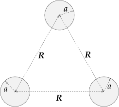
Figure 6.1: The three-disk system with center-to-center separation $R=6a$.

The genuine multiscattering data in the ${\rm A}_{\rm 1}$ subspace are computed from the determinant ${\rm det}[1+{\bf A}_{{\rm A}_{\rm 1}}(k)]$ where the multiscattering kernel ${\bf A}_{{\rm A}_{\rm 1}}(k)$, expressed in the angular momentum basis relative to the half-disk in the fundamental regime, reads [13]

$${\bf A}_{{\rm A}_{\rm 1}}(k)_{m,m^{\prime}} = d(m)d(m^{\prime})\frac{J_{m}(ka)}{H^{(1)}_{m^{\prime}}(ka)}\left\{\cos\left(\frac{\pi}{6}(5m-m^{\prime})\right)H^{(1)}_{m-m^{\prime}}(kR)\right.$$ (6.1)

$$\qquad\mbox{}\left.+(-1)^{m^{\prime}}\cos\left(\frac{\pi}{6}(5m+m^{\prime})\right)H^{(1)}_{m+m^{\prime}}(kR)\right\}$$

with $0\leq m,m^{\prime}<\infty$ and

$$d(m):=\left\{\begin{array}[]{ccc}\sqrt{2}&{\rm for}&m>0\\ 1&{\rm for}&m=0\ .\end{array}\right.$$ (6.4)

As ${\bf A}$ is trace-class for any $n$-disk geometry, the determinant exists and can numerically be calculated in a truncated Hilbert space. The Hilbert space is here the space of angular momentum eigenfunctions $\{|m\rangle\}$ on the surface of the half-disk in the fundamental domain which can be truncated by an upper angular momentum $m_{\rm max}$. From the study, in App.C, of the asymptotic behaviour of ${\bf A}_{m,m^{\prime}}$ with respect to the angular momentum one can derive the following inequality for the truncation point $m_{\rm max}$:

$$m_{\rm max}\mbox{\raisebox{-2.58334pt}{$\,{\stackrel{{\scriptstyle>}}{{\sim}}}\,$}}\frac{e}{2}ka\approx 1.5ka\;.$$ (6.5)

This agrees, of course, with the numerical findings. The truncated matrix ${\bf M}_{{\rm A}_{\rm 1}}(k)$ is then numerically transformed to an upper triangular matrix and the determinant is calculated from the product of the diagonal elements. This procedure is faster than the computation of the determinant from the product of the eigenvalues of ${\bf M}_{{\rm A}_{\rm 1}}(k)$ (see (A.10)). The numerical results for both ways agree, of course, up to computer accuracy. The zeros of the determinant, ${\rm det}{\bf M}_{{\rm A}_{\rm 1}}(k)$, in the lower complex wave-number plane determine the scattering resonances, whereas the phase of the determinant evaluated on the real $k$-axis gives the cluster phase shift. The cumulants can be constructed either from the Plemelj-Smithies recursion formula (A.14) or from the multinomials of the eigenvalues (A.11). The latter procedure is numerically more stable, especially deep inside the negative complex wave-number plane. This concludes the numerical setup for the exact calculation.

As shown in Secs.4 and 5 the classical analog of the characteristic determinant (actually of ${\rm det}\{{\bf 1}+z{\bf A}(k)\}$ to be precise) is the semiclassical zeta function of Gutzwiller [5] and Voros [37] which, prior to a regularization, is given by $Z_{GV}(z;k)$ (see (2.1)). However, in the literature there exist other competitors for a semiclassical zeta function, e.g., the dynamical zeta function $\zeta_{0}^{-1}(z;k)$ of Ruelle[36] (see (2.2)) which is the $j$=0 part of the Gutzwiller-Voros zeta function as well as the quasiclassical zeta-function $Z_{\rm qcl}(z;k)$ of ref.[43] (see (2.3)). As usual, for all three choices, $t_{p}(k)={\e^{{\rm i}kL_{p}-{\rm i}\nu_{p}\pi/2}}/{|\Lambda_{p}|^{{\textstyle\frac{1}{2}}}}$ is the $p^{\,\rm th}$ primary cycle, $n_{p}$ its topological length, $L_{p}$ is its geometrical length, $\nu_{p}$ its Maslov index together with the group theoretical weight of the studied ${\rm C}_{\rm 3v}$-representation (in the present case the ${\rm A}_{\rm 1}$-representation), and $\Lambda_{p}$ its stability (the expanding eigenvalues of the stability matrix) — see refs.[42, 43] for further details. The variable $z$ is a book-keeping device for keeping track of the topological order in the cycle- or curvature expansion [18, 19] (see Eqs.(2) and (4.9)). In the following, the various curvature-expanded zeta functions are truncated at a given curvature (i.e., total topological) order $n_{c}$. The semiclassical predictions for the scattering resonances are determined from the zeros of these truncated zeta functions, the predictions for the cluster phase shifts discussed in Sec.6.2 from the phases on the real $k$-axis and the curvatures from the terms of order $z^{m}$ in the curvature expansion. Input data for the lengths $L_{p}$ , stabilities $\Lambda_{p}$ and Maslov indices $\nu_{p}$ of the periodic orbits of the 3-disk system in the ${\rm A}_{\rm 1}$-representation have been taken from Rosenqvist [68, 69], Scherer [17] and Eckhardt [70].

6.1 Exact versus semiclassical resonances

In this chapter we compare the numerically computed exact quantum-mechanical resonances of the 3-disk repeller with the corresponding semiclassical predictions of the three semiclassical zeta functions: the Gutzwiller-Voros zeta function (2.1), the dynamical zeta function (2.2) and the quasiclassical zeta function (2.3).

For the 3-disk-repeller with center-to-center separation $R\mbox{=}6a$, we have computed all exact quantum-mechanical ${\rm A}_{\rm 1}$ resonances (numerically determined from the zeros of ${\rm det}{\bf M}_{{\rm A}_{\rm 1}}(k)$) as well as all the corresponding approximate ones (from the zeros of the at finite curvature order $n_{c}$ truncated zeta functions) in the wave-number window: $0\leq{\rm Re}\,k\leq 250/a$ and $0\geq{\rm Im}\,k\geq-1.6/a$. This window contains several hundreds of leading and subleading resonances, from the lowest ones onwards. In Figs. G.1–G.9, for increasing curvature order, the resonances are plotted as the real part of the wave number (resonance “energy”) versus the imaginary part of the wave number (resonance “width”).

Some features of the resonance spectra allow for an immediate interpretation [13, 17, 15]: The mean spacing of the resonances is approximately $2\pi/{\bar{L}}$, where ${\bar{L}}$ is the average of the geometrical lengths of the shortest periodic orbits, namely the lengths $L_{0}$ and $L_{1}$ of the two periodic orbits of topological length one. The data also exhibit various beating patterns resulting from the interference of the periodic orbits of nearly equal length; e.g., the leading beating pattern is of order $2\pi/{\Delta L}$, where $\Delta L$ is the difference of the lengths $L_{1}$ and $L_{0}$.

In Figs. G.1 – G.4 a comparison is made from the first- up to the fourth order in the curvature expansion. Already at fourth order the four leading resonance bands are well approximated by the Gutzwiller-Voros zeta-function (in fact, for ${\rm Re}\,k\mbox{\raisebox{-2.58334pt}{$\,{\stackrel{{\scriptstyle<}}{{\sim}}}\,$}}75/a$ already the second curvature order is enough to describe the first two leading resonance bands). This is in agreement with the rule of thumb that any new resonance band is linked with a new curvature or cumulant order. Neither the dynamical zeta-function nor the quasiclassical one perform as well to fourth order. The reason is that the quasiclassical as well as the dynamical zeta-function predict extra resonances which are absent in the exact quantum-mechanical calculation. Thus the third and fourth curvature order of these zeta-functions are distributed over the average of the third and fourth resonance bands and the spurious extra resonances. In the window plotted one can classify the exact data into four leading resonance bands closest to the real wave-number axis and 2 subleading ones shielded by the leading resonances. Thus, just periodic orbits of topological length up to four are needed in order to reproduce the qualitative trend of the exact data closest to the real axis. The 3-disk-system has 8 periodic orbits up to this topological length. Actually, the 3-disk-system with center-to-center separation $R=6a$ is not very chaotic at these $k$ values. All experimentally accessible spectral data in this regime (which can be extended up to ${\rm Re}\,k\approx 950/a$ as only about there the subleading resonance bands mix with the four leading ones) can be parameterized by 16 real numbers, i.e., 8 periodic orbit lengths, 8 stabilities, and 8 Maslov indices. Experimentalists can stop here. The subleading bands are completely shielded (up to ${\rm Re}\,k\approx 950/a)$ by the above mentioned four bands. The subleading bands (below ${\rm Re}\,k\approx 950/a$) are only of theoretical interest, as they can be used to test the semiclassical zeta functions.

In Figs. G.5 a comparison is made up to fifth curvature order. The Gutzwiller-Voros zeta-function does at least as well as in Fig. G.4a for the leading four resonance bands, but now it also describes the peak position of the fifth resonance band for large enough values of ${\rm Re}\,k$. Note the diffractive band of exact resonances from $k\approx(0.-{\rm i}0.5)/a$ to $k\approx(100.-{\rm i}1.6)/a$ which our semiclassical zeta functions fail to describe. As shown in Refs.[32, 33, 34] the diffractive band of resonances can be accounted for by inclusion of creeping periodic orbits which have been omitted from our semiclassical calculations. The dynamical and quasiclassical zeta functions show a slight improvement with respect to the four leading resonance bands; however, no agreement with the fifth one.

In Figs. G.6 a comparison is made up to sixth curvature order. The Gutzwiller-Voros zeta-function fails for the third resonance band below ${\rm Re}\,k\approx 20/a$, for the fourth below ${\rm Re}\,k\approx 45/a$, for the fifth and sixth below ${\rm Re}\,k\approx 70/a$ and 80/$a$, respectively. Below these values, the last two curvature orders try to build up an accumulation line. Above these values, the qualitative agreement with the data is rather good. The dynamical zeta-functions at this order just improves the description of the four leading resonance bands. Furthermore, it builds up a sharp line of accumulation for the subleading resonances, the border of convergence controlled by the location of the nearest poles of the dynamical zeta function, see [41, 42]. The quasiclassical zeta function also improves the description of the four resonance bands, although it is still not of the same quality as the Gutzwiller-Voros one even at two curvature orders lower. Note that the quasiclassical zeta function is trying to build up two bands of spurious resonances in agreement with our rule of thumb.

In Figs. G.7 a comparison is made up to seventh curvature order. The first four resonance bands of the Gutzwiller-Voros zeta function have converged and the accumulation line has moved up. Only above ${\rm Re}\,k\approx 140/a$ the fifth and sixth resonance band emerge, now with improved accuracy, however. Also the seventh resonance band is approximated. The dynamical zeta-function now clearly produces its line of convergence (the accumulation line of resonances). Above this line, the resonances (except the ones very close to the accumulation) are approximated as well as in the Gutzwiller-Voros case; below, no agreement is found. At this order the quasiclassical zeta-function is doing as well as the Gutzwiller-Voros zeta-function did already at curvature order four. None of the subleading bands are described by the quasiclassical zeta-function. Instead another band of spurious resonances emerges.

In Figs. G.8 and G.9 the comparison is made up to the eighth and twelfth curvature order, respectively. The border of convergence of the Gutzwiller-Voros zeta-function has now moved (in the plotted region) above the fifth and sixth band of the exact resonances. It has moved also closer to the very sharp accumulation line of resonances of the dynamical zeta function. However, these lines are still not identical even at twelfth curvature order. The subleading quasiclassical resonances have stabilized onto the spurious bands. Furthermore, some subleading resonances move further down into the lower complex $k$-plane . Eventually (see also [68]), starting with curvature order 10 and 12 the fifth and sixth resonance bands are approximated — in addition, to four or six spurious resonance bands, respectively. Thus the quasiclassical zeta-function seems to find the subleading resonance bands, but at the cost of many extra spurious resonances. Note that at these high curvature orders the quasiclassical zeta-function has numerical convergence problems for large negative imaginary $k$ values (especially for low values of ${\rm Re}\,k$). This is in agreement with the expected large cancellations in the curvature expansion at these high curvature orders. Furthermore, periodic orbits of larger topological order than twelve would be needed to falsify the success of the quasiclassical zeta function, since it barely manages to approximate the two bands of subleading resonances at this curvature order.

Qualitatively, the results can be summarized as follows. The Gutzwiller-Voros zeta-function does well above its line of convergence, defined by the dynamical zeta-function, already at very low curvature orders where the dynamical zeta-functions still has problems. Below this line we observe that the Gutzwiller-Voros zeta-function works only as an asymptotic expansion. However, when it works, it works very well and very efficiently. This implies that the additional ($\Lambda_{p}$-dependent) terms of the Gutzwiller-Voros zeta function, relative to the simpler dynamical zeta function, are the correct ones. This is of course in agreement with the findings of our semiclassical reduction in Sec.5. Eventually, the dynamical zeta-function does as well for the leading resonances as the Gutzwiller-Voros one. As experimentally these are the only resonances accessible, one might – for practical purposes – limit the calculation just to this zeta function, see, however, Sec.6.2. The quasiclassical zeta-function seems to find all subleading geometrical resonances. Unfortunately, the highest periodic orbits at our disposal are of topological length 12; the very length where the sixth resonance band seems to emerge. Thus higher orbits would be needed to confirm this behavior. But all this comes at a very high price: The rate of convergence is slowed down tremendously (in comparison with the asymptotically working Gutzwiller-Voros zeta-function), as this zeta-function is producing additional spurious resonance bands which do not have quantum-mechanical counter parts, but only classical ones [47]. Without a quantum calculation, one could therefore not tell the spurious from the real resonances.

As a by-product we have a confirmation of our empirical rule of thumb that ‘each new cumulant or curvature order is connected with a new line of subleading resonances’. This rule therefore relates the curvature truncation limit, $m\to\infty$, either to the limit ${\rm Im}\,k\to-\infty$, if there is no accumulation of subleading resonances, i.e., if the zeta function is entire [42, 43], or to the formation of an accumulation band of resonances. Both facts support our claim that, in general, the curvature limit $m\to\infty$ and the semiclassical limit ${\rm Re}\,k\to\infty$ cannot and should not commute deep inside the lower complex $k$-plane, as the subleading resonances of increasing cumulant order are approximated worse and worse. Only an asymptotic expansion should be possible, in agreement with our findings for the Gutzwiller-Voros zeta function.

6.2 Exact versus semiclassical cluster phase shifts

In the last chapter the semiclassical zeta functions were judged by the comparison of their resonances predictions with the exact resonances poles (especially the subleading ones), as was done in the past, see e.g. Refs.[13, 15, 42, 44, 45, 32, 34]. Since the deviations between the zeta functions themselves and from the exact data are most pronounced for the subleading resonances (which are shielded by the leading ones), one could argue that empirically it does not matter which of the three zeta functions are used to describe the measured data, since all three give the same predictions for the leading resonances [42, 43].

Below, however, we will show that even experimentally one can tell the three semiclassical zeta functions apart and that, in fact, the Gutzwiller-Voros one is by far the best.

6.2.1 Cluster phase shifts

In Sec.4 the exact and semiclassical expressions for the determinant of ${\bf S}$-matrix for non-overlapping $n$-disk systems have been constructed. For the case of the 3-disk system they read

$${\rm det}_{{l}}{\bf S}^{(3)}(k) = \left({\rm det}_{{l}}{\bf S}^{(1)}(ka)\right)^{3}\frac{{\rm det}_{{l}}{{\bf M}_{{\rm A}_{\rm 1}}(k^{\ast})}^{\dagger}}{{\rm det}_{{l}}{\bf M}_{{\rm A}_{\rm 1}}(k)}\,\frac{{\rm det}_{{l}}{{\bf M}_{{\rm A}_{\rm 2}}(k^{\ast})}^{\dagger}}{{\rm det}_{{l}}{\bf M}_{{\rm A}_{\rm 2}}(k)}\,\frac{\left({{\rm det}_{{l}}{\bf M}_{\rm E}(k^{\ast})}^{\dagger}\right)^{2}}{\left({\rm det}_{{l}}{\bf M}_{\rm E}(k)\right)^{2}}$$

$$\ \stackrel{{\scriptstyle\rm s.c.}}{{\longrightarrow}}\ \left(\e^{-{\rm i}\pi N(k)}\right)^{2\times 3}\,\left(\frac{{{\widetilde{Z}}_{\rm 1\mbox{-}disk(l)}(k^{\ast})}^{\ast}}{{{\widetilde{Z}}_{\rm 1\mbox{-}disk(l)}(k)}}\,\frac{{{\widetilde{Z}}_{\rm 1\mbox{-}disk(r)}(k^{\ast})}^{\ast}}{{{\widetilde{Z}}_{\rm 1\mbox{-}disk(r)}(k)}}\right)^{3}\times$$

$$\qquad\qquad\qquad\times\frac{{{\widetilde{Z}}_{{\rm A}_{\rm 1}}(k^{\ast})}^{\ast}}{{\widetilde{Z}}_{{\rm A}_{\rm 1}}(k)}\,\frac{{{\widetilde{Z}}_{{\rm A}_{\rm 2}}(k^{\ast})}^{\ast}}{{\widetilde{Z}}_{{\rm A}_{\rm 2}}(k)}\,\frac{{{{\widetilde{Z}}_{{\rm E}}(k^{\ast})}^{\ast}}^{2}}{{{\widetilde{Z}}_{{\rm E}}(k)}^{2}}$$

where the tilde indicates that diffractive corrections have to be included, in general. Especially for the ${\rm A}_{\rm 1}$-representation of the 3-disk system we therefore have the relation between the quantum-mechanical kernels and the Gutzwiller-Voros zeta functions

$$\frac{{\rm det}_{{l}}{{\bf M}_{{\rm A}_{\rm 1}}(k^{\ast})}^{\dagger}}{{\rm det}_{{l}}{\bf M}_{{\rm A}_{\rm 1}}(k)}\ \stackrel{{\scriptstyle\rm s.c.}}{{\longrightarrow}}\ \frac{{{Z}_{{\rm A}_{\rm 1}}(k^{\ast})}^{\ast}}{{Z}_{{\rm A}_{\rm 1}}(k)}\ ,$$ (6.7)

where we have now neglected diffractive corrections. As argued in the conclusion section 7 both sides of Eq.(LABEL:3disk-link) and Eq.(6.7) respect unitarity; the quantum-mechanical side exactly and for the semiclassically side under the condition that the curvature expansion converges or that it is truncated. As all the $n$-disk resonances for non-overlapping $n$-disk repellers are below the real $k$-axis, the border of absolute convergence, defined by the closest resonances to the real axis [15, 42] is inside the lower complex wave-number plane and unitarity on the real axis is guaranteed. Thus, if the wave number $k$ is real, the left hand sides and also the right hand sides of eqs.(LABEL:3disk-link) and (6.7) can be written as $\exp\{{\rm i}2\eta(k)\}$ with a real phase shift $\eta(k)$. In fact, we can define a total phase shift for the coherent part of the 3-disk scattering problem (here always understood in the ${\rm A}_{\rm 1}$-representation) for exact quantum mechanics as well as for the three semiclassical candidates by:

$$\e^{2{\rm i}\eta_{\rm qm}(k)} := \frac{{\rm det}_{{l}}{{\bf M}(k^{\ast})}^{\dagger}}{{\rm det}_{{l}}{\bf M}(k)}$$ (6.8)

$$\e^{2{\rm i}\eta_{\rm GV}(k)} := \frac{{{Z}_{\rm GV}(k^{\ast})}^{\ast}}{{Z}_{\rm GV}(k)}$$ (6.9)

$$\e^{2{\rm i}\eta_{\rm dyn}(k)} := \frac{{\zeta_{0}^{-1}(k^{\ast})}^{\ast}}{\zeta_{0}^{-1}(k)}$$ (6.10)

$$\e^{2{\rm i}\eta_{\rm qcl}(k)} := \frac{{{Z}_{qcl}(k^{\ast})}^{\ast}}{{Z}_{qcl}(k)}\ .$$ (6.11)

This phase shift definition should be compared with the cluster phase shift given in Sec. 4 of Lloyd and Smith [53]. For a separable system, as e.g. the 1-disk system (in the angular momentum representation), the cluster phase shift just corresponds to the sum

$$\eta(k)=\sum_{l=-\infty}^{\infty}\eta_{l}(k)\ ,$$ (6.12)

as the ${\bf S}$-matrix of the one-disk system (evaluated with respect to the center of the disk) reads

$${\bf S}_{ll^{\prime}}(k) = \frac{-H^{(2)}_{l}(ka)}{H^{(1)}_{l}(ka)}\delta_{ll^{\prime}}$$ (6.13)

$$= \e^{2{\rm i}\eta_{l}(k)}\delta_{ll^{\prime}}\ ,$$

such that

$${\rm det}{\bf S}(k)=\prod_{l=-\infty}^{+\infty}\e^{2{\rm i}\eta_{l}(k)}\ .$$ (6.14)

Let us once more stress: the coherent or cluster phase shift is an experimentally accessible quantity: from the measured differential cross sections the elastic scattering amplitudes have to be constructed. This leads to the full phase shift of the 3-disk system including the contribution from the single disks. However, the incoherent part can be subtracted by either making reference experiments with just single disks at the same position where they used to be in the 3-disk problem or by numerical subtractions as the one-disk phase shifts are known analytically, since the system is separable, see (6.13) and (6.14). In this way one can separate the incoherent phase shifts from the coherent ones.

Thus $\eta_{\rm qm}(k)$ is “measurable” in principle. We next use these cluster phase shifts in order to discriminate between the various zeta functions. Below, we compare the exact quantum-mechanical cluster phase shift $\eta_{qm}$ with

1. the semiclassical cluster phase shift $\eta_{\rm GV}(k)$ of the Gutzwiller-Voros zeta function (2.1),

2. with the semiclassical cluster phase shift $\eta_{\rm dyn}(k)$ of the dynamical zeta function (2.2),

3. and with the semiclassical cluster phase shift $\eta_{\rm qcl}(k)$ of the quasiclassical zeta function (2.3).

The zeta functions in the numerator as well as in the denominator of $Z(k)^{\ast}/Z(k)$ have been expanded to curvature order (=topological length) 12. For the Gutzwiller-Voros zeta function this is an overkill as already curvature order 4 should describe the data below ${\rm Re}k=950/a$. In fact, we have not seen any difference in the Gutzwiller-Voros calculation between the curvature order 3 and 12 results for $k\leq 120/a$ and up to figure accuracy. Curvature order 2, however, gives in the regime $100/a\leq k\leq 120/a$ noticeable deviations. On the other hand, as mentioned in Sec.6.1, the quasiclassical zeta function has problems for lower curvature orders with predicting the (sub-)leading resonances; therefore, these high curvature orders are used in order to give the quasiclassical zeta function as fair a chance as possible. The coherent phase shifts are compared in the window $104/a\leq k\leq 109/a$, which is a typical window narrow enough to resolve the rapid oscillations with $k$ sufficiently large such that diffractive effects can be safely neglected. Furthermore, although we have no physical interpretation in terms of the ${\bf S}$-matrix, we also compare in the same window the exact quantum-mechanical product ${\rm det}{\bf M}(k){\rm det}{\bf M}(k^{\ast})^{\dagger}$ with the squared modulus of the Gutzwiller-Voros zeta function $Z_{\rm GV}(k)Z_{\rm GV}(k^{\ast})^{\ast}$, the dynamical zeta function $\zeta_{0}^{-1}(k)\zeta_{0}^{-1}(k^{\ast})^{\ast}$, and the quasiclassical zeta function $Z_{\rm qcl}(k)Z_{\rm qcl}(k^{\ast})^{\ast}$. Here $k$ is taken to be real and the case of the 3-disk system in the ${\rm A}_{\rm 1}$-representation with center-to-center separation $R=6a$ is studied.

Consider finally the general quasiclassical zeta functions of Ref.[43] and especially the ratio

$$Z(k):=\frac{F_{+}({\textstyle\frac{1}{2}},k)F_{-}({7\over 2},k)}{F_{-}({\textstyle\frac{3}{2}},k)F_{+}({5\over 2},k)}$$ (6.15)

with $F_{+}(\beta,k;z)$ and $F_{-}(\beta,k;z)$ being defined as follows

$$F_{+}(\beta,k;z) = \exp\left\{-\sum_{p}\sum_{r=1}^{\infty}\frac{1}{r}\frac{\left(z^{[p]}\,t_{p}(k)\right)^{r}}{\left(1-\frac{1}{\Lambda_{p}^{r}}\right)^{2}\left(1-\frac{1}{\Lambda_{p}^{2r}}\right)}|\Lambda_{p}^{r}|^{-\beta+{\textstyle\frac{1}{2}}}\right\}$$

$$F_{-}(\beta,k;z) = \exp\left\{-\sum_{p}\sum_{r=1}^{\infty}\frac{1}{r}\frac{\Lambda_{p}^{r}}{|\Lambda_{p}^{r}|}\,\frac{\left(z^{[p]}\,t_{p}(k)\right)^{r}}{\left(1-\frac{1}{\Lambda_{p}^{r}}\right)^{2}\left(1-\frac{1}{\Lambda_{p}^{2r}}\right)}|\Lambda_{p}^{r}|^{-\beta+{\textstyle\frac{1}{2}}}\right\}\;.$$

Here the subleading factor $(1+|\Lambda_{p}^{r}|^{2\beta-4})$ of Eq.(11) in ref.[43] has been removed as in Eq.(12) of ref.[43]. When Eq.(6.15) is used, the corresponding coherent phase shift

$$\e^{{\rm i}2\eta_{\rm rat}(k)}=\frac{Z(k^{\ast})^{\ast}}{Z(k)}$$ (6.16)

works on the real wave-number axis and in the limit $n\to\infty$ (where $n$ is the curvature order) as well as the original Gutzwiller-Voros zeta function. Hence, it does not matter here whether the Gutzwiller-Voros zeta function is directly expanded in the curvature expansion or whether the individual determinants $F_{+}({\textstyle\frac{1}{2}},k)$, $F_{-}({7\over 2},k)$, $F_{-}({\textstyle\frac{3}{2}},k)$ and $F_{+}({5\over 2},k)$ are each expanded in separate curvature expansions up to the same curvature order and then inserted in the ratio (6.15). Note that the presence or absence of the subleading factor $(1+|\Lambda_{p}^{r}|^{2\beta-4})$ in the definitions of $F_{+}(\beta,k;z)$ and $F_{-}(\beta,k;z)$ does not change the results up to figure accuracy.

(a)

(b)

Figure 6.2: (a) The coherent cluster phase shifts of the 3-disk scattering system in the ${\rm A}_{\rm 1}$-representation with center-to-center separation $R=6a$. The exact quantum-mechanical data are compared to the predictions of the Gutzwiller-Voros zeta function (2.1), the dynamical zeta function (2.2) and the quasiclassical zeta function (2.3) calculated up to 12th order in the curvature expansion. (b) The same for the squared moduli of the exact spectral determinant and the semiclassical zeta functions. The predictions of the Gutzwiller-Voros zeta function and exact quantum mechanics coincide within the resolutions of the plots.

Let us stress that phase shifts are not only of theoretical interest, as are the subleading resonances (which are completely shielded by the leading resonances), but hard data which can be extracted, in principle, from measured differential cross sections.

In summary, even empirically, one can tell the three semiclassical zeta functions apart and see which is the best. Again the Gutzwiller-Voros one — whether used directly or whether defined as the ratio (6.15) of four quasiclassical determinants as in ref.[43] — is by far the best.

6.3 The quantum-mechanical cumulant expansion versus the semiclassical curvature expansion

In this subsection it will be shown that the Gutzwiller-Voros zeta function approximates its quantum-mechanical counterpart, the characteristic KKR-type determinant [51, 53, 49], only in an asymptotic sense, such that it always should be understood as a truncated series.

As shown in Sec.4, the characteristic determinant and the Gutzwiller-Voros zeta-function are related as

$${\rm det}{\bf M}(k)\ \stackrel{{\scriptstyle\rm s.c.}}{{\longrightarrow}}\ Z_{\rm GV}(k)\;.$$ (6.17)

Let $Q_{m}(k)$ denote the $m^{\,\rm th}$ cumulant of ${\rm det}{\bf M}(k)$ – i.e. the term proportional to $z^{m}$ in the Taylor expansion of ${\rm det}\{{\bf 1}+z{\bf A}(k)\}$ – which satisfies the Plemelj-Smithies recursion relation (4.6) (see also App.A). Since the Plemelj-Smithies recursion formula is plagued by cancellations of very large numbers, we have not used the Plemelj-Smithies recursion relations for our numerical calculation of $Q_{m}(k)$, but instead we construct this quantity directly from the eigenvalues $\{\lambda_{j}(k)\}$ of the trace-class matrix ${\bf A}(k)$, i.e.

$$Q_{m}(k)=\sum_{1\leq j_{1}<\cdots<j_{m}<\infty}\lambda_{j_{1}}(k)\cdots\lambda_{j_{m}}(k)$$ (6.18)

(see again App.A for more details). Unfortunately, a semiclassical analog to this exact formula has not been found so far. Thus $C_{m}(k)$, the corresponding semiclassical $m$th-order curvature term, of $Z_{\rm GV}(k)$, can only be constructed from the semiclassical equivalent of the Plemelj-Smithies recursion relation (4.8) which exactly corresponds to the standard curvature expansion of refs.[19, 42, 15]) and is therefore inherently plagued by large cancellations. The cumulant and curvature expansions, truncated at $n$th order, read:

$${\rm det}{\bf M}(k)|_{n} = \sum_{m=0}^{n}Q_{m}(k)$$ (6.19)

$$Z_{\rm GV}(k)|_{n} = \sum_{m=0}^{n}C_{m}(k)\ .$$ (6.20)

Let us recapitulate what we already know about these series. From Sec.4 together with the appendices A and C we deduce that the cumulant sum

$$\lim_{n\to\infty}{\rm det}{\bf M}(k)|_{n}=\lim_{n\to\infty}\sum_{m=0}^{n}Q_{m}(k)={\rm det}{\bf M}(k)$$ (6.21)

is absolutely convergent, i.e.

$$\sum_{m=0}^{\infty}|Q_{m}(k)|<\infty\ ,$$ (6.22)

because of the trace-class property of ${\bf A}(k)\equiv{\bf M}(k)-{\bf 1}$ for non-overlapping, disconnected $n$-disk systems. On the other hand, as discussed in Refs.[41, 42, 43], the Gutzwiller-Voros curvature sum converges only above an accumulation line (running below and approximately parallel to the real wave-number axis, see Sec.6.1) which is given by the first poles of the dynamical zeta function, $\zeta_{0}^{-1}(k)$, or the leading zeros of the subleading zeta function. However, as shown in Sec.6.1, even below this boundary of convergence the truncated Gutzwiller-Voros curvature sum, $Z_{\rm GV}(k)|_{n}$ approximates the quantum-mechanical data as an asymptotic series.

In addition, a very important property for the discussion of the cumulant and curvature terms is the existence of the scaling formulas (established by us numerically) which relate the $m$th cumulants or curvatures inside the complex wave-number plane to the corresponding quantities on the real $k$-axis:

$$Q_{m}({\rm Re}\,k+{\rm i}{\rm Im}\,k) \sim Q_{m}({\rm Re}\,k)\e^{-m\bar{L}{\rm Im}\,k}$$ (6.23)

$$C_{m}({\rm Re}\,k+{\rm i}{\rm Im}\,k) \sim C_{m}({\rm Re}\,k)\e^{-m\bar{L}{\rm Im}\,k}\ .$$ (6.24)

(For this to hold, diffractive effects have to be negligible, i.e. $-{\rm Im}\,k\ll{\rm Re}\,k$.) Here $\bar{L}\approx R-2a$ is the average of the geometrical lengths of the shortest periodic orbits, the two orbits of topological length one. The scaling can be motivated by the approximate relation ${\rm Tr}[{\bf A}^{m}(k)]\approx\{{\rm Tr}{\bf A}(k)\}^{m}$ which, of course, cannot be exact, as otherwise the cumulants would be identically zero. Nevertheless, the overall behaviour follows from this, since

$${\rm Tr}\left[{\bf A}({\rm Re}\,k+{\rm i}{\rm Im}\,k)\right]\ \sim{\rm Tr}\left[{\bf A}({\rm Re}\,k)\right]\e^{-\bar{L}{\rm Im}\,k}\;.$$

From Fig.6.3 one can deduce that the deviations between quantum-mechanical cumulants and semiclassical curvatures (as evaluated on the real $k$-axis) decrease with increasing ${\rm Re}\,k$, but increase with increasing curvature order $m$. The value of ${\rm Re}\,k$ where the quantum-mechanical and semiclassical curves join is approximately given by ${\rm Re}\,ka\sim 2^{m+1}$. Approximately the same transition points can be generated from a comparison of the phases of the cumulant and curvatures.

Figure 6.3: Comparison of the squared moduli (on a logarithmic scale) of the first seven quantum-mechanical cumulant terms, $|Q_{n}(k)|^{2}$, with the corresponding semiclassical curvature terms, $|C_{n}(k)|^{2}$, of the Gutzwiller-Voros zeta function (2.1) evaluated on the real wave-number axis $k$. The system is the ${\rm A}_{\rm 1}$ three-disk repeller with center-to-center separation $R=6a$.

By varying the center-to-center distance we have numerically verified that the above limits generalize to the following relations valid on the real wave-number axis ($k$ real and positive):

$$C_{m}(k)\approx Q_{m}(k)\quad{\rm with}\ \ 1\gg|C_{m}(k)|\approx|Q_{m}(k)|\qquad{\rm if}\ \ ka\mbox{\raisebox{-2.58334pt}{$\,{\stackrel{{\scriptstyle>}}{{\sim}}}\,$}}\,2^{m-1}\frac{\bar{L}}{a}$$ (6.25)

and

$$1\gg|C_{m}(k)|\gg|Q_{m}(k)|\qquad{\rm if}\ \ ka\mbox{\raisebox{-2.58334pt}{$\,{\stackrel{{\scriptstyle<}}{{\sim}}}\,$}}\,2^{m-1}\frac{\bar{L}}{a}\;.$$ (6.26)

What is the interpretation of (6.25) and (6.26)? For fixed $k$, even in the regime, where $Z_{\rm GV}(k)|_{n}$ converges, e.g., on the real $k$-axis, the Gutzwiller-Voros zeta function is only an asymptotic approximation to the true quantum-mechanical cumulant sum, since for $m>m_{\rm crit}$, defined by $ka\approx 2^{m_{\rm crit}-1}\frac{\bar{L}}{a}$, the exact quantum-mechanical cumulants $Q_{m}(k)$ and the semiclassical curvatures $C_{m}(k)$ are grossly different. These deviations can be enhanced by the $m^{\,{\rm th}}$ derivative, $m>m_{\rm crit}$, with respect to the book-keeping variable $z$, since this operation eliminates all approximately equal terms, such that the corresponding cumulant and curvature series are transformed to completely different expressions. The fact that $Z_{\rm GV}(k)|_{n}$ – even in its convergence regime – is only an asymptotic expansion to the exact quantum mechanics is normally not visible, as the terms in (6.25) are exponentially small on or close to the real axis and therefore sum to a tiny quantity. In other words, close to the real axis the absolute error $|C_{n}(k)-Q_{n}(k)|$ for $m>m_{\rm crit}$ is still small. The relative error $|C_{n}(k)/Q_{n}(k)|$ on the other hand is tremendous (see Fig.6.3). Deeper inside the negative complex wave-number plane, however, under the scaling rules (6.23) and (6.24), the deviations (6.26) are blown up, such that the relative errors $|C_{n}(k)/Q_{n}(k)|$ eventually become visible as absolute errors $|C_{n}(k)-Q_{n}(k)|$ in the resonance calculation of Sec.6.1. If ${\rm Im}\,k$ is above the boundary line of convergence, these errors still sum up to a finite quantity which might, however, not be negligible any longer, as was the case on or close to the real $k$-axis. Below the convergence line these errors sum up to infinity. Thus the Gutzwiller-Voros curvature expansion $Z_{\rm GV}(k)|_{n}$ does not suddenly become an asymptotic approximation to ${\rm det}{\bf M}(k)|_{n}$, it always is an asymptotic approximation (as shown by the relative error $|C_{n}(k)/Q_{n}(k)|$), even in its convergence regime above the accumulation line and even on the real axis, where the zeta function itself is in its domain of absolute convergence [17].

Thus, the value of ${\rm Im}\,k$ where — for a given $m$ — the $Z_{\rm GV}(k)|_{n}$ sum deviates from ${\rm det}{\bf M}(k)|_{n}$ is governed by the real part of $k$ and the scaling rules (6.23) and (6.24). It has nothing to do with the boundary line between the convergence region and the asymptotic region of $Z_{\rm GV}(k)$, as the asymptotic expansion is given by a finite sum of all terms satisfying (6.25). Therefore, the truncated Gutzwiller-Voros expansion describes the quantum-mechanical resonance data even below the line of convergence of the infinite curvature series, see 6.1. On the other hand, the boundary line of the convergence regime of the Gutzwiller-Voros expansion is solely governed by those $C_{m}(k)$ which have nothing to do with the quantum analog $Q_{m}(k)$, i.e. solely by terms of character (6.26). The reason is, of course, that the convergence property of an infinite sum is governed by the infinite tail and not by the first few terms. Whether the Gutzwiller-Voros expansion converges or not is therefore not related to whether the quantum-mechanical data are described well or not.

The convergence property of a semiclassical zeta function on the one hand and the approximate description of quantum mechanics by these zeta functions are two different things. It could happen that a zeta function is convergent, but not a good description of quantum mechanics (see especially the failure of the entire quasiclassical zeta function to approximate the exact cluster phase shift in Sec.6.2). On the other hand it may not converge, in general, but its finite truncations nevertheless approximate – at least to some order – quantum mechanics, as it is the case for the Gutzwiller-Voros zeta function.

These findings hold for any re-writing of the Gutzwiller-Voros zeta function, as $Z_{\rm GV}(k)|_{n}$ was already shown to be asymptotic in a regime where the curvature sum is still absolutely convergent and the limit $\lim_{n\to\infty}Z_{\rm GV}(k)|_{n}$ exists. Therefore, any re-writing of $Z_{\rm GV}(k)$, especially the one of ref.[43] as the ratio of four quasiclassical zeta functions (6.15) will at best work as an asymptotic expansion to the exact quantum-mechanical cumulant expansion. Note that, for finite curvature order $n$

$$\frac{F_{+}({\textstyle\frac{1}{2}},k)|_{n}F_{-}({7\over 2},k)|_{n}}{F_{-}({\textstyle\frac{3}{2}},k)|_{n}F_{+}({5\over 2},k)|_{n}} \neq \left.\left\{\frac{F_{+}({\textstyle\frac{1}{2}},k)F_{-}({7\over 2},k)}{F_{-}({\textstyle\frac{3}{2}},k)F_{+}({5\over 2},k)}\right\}\right|_{n}$$

$$= Z_{\rm GV}(k)|_{n}\ .$$

If the ratio is evaluated according to the r.h.s. of (6.3), one obtains exactly the same result as for the original Gutzwiller-Voros expansion using formula (2.1). If, however, the ratio is evaluated according to l.h.s. of (6.3), the relation to the quantum-mechanical cumulant expansion is lost: the matching of the semiclassical coefficients of $z^{m}$ with the quantum-mechanical ones is spoiled, as the asymptotic terms, resulting from various curvature orders of the $Z_{\rm GV}(k)|_{n}$ calculation, mix. If $n$ is large enough, also the l.h.s. of (6.3) will deviate strongly from the quantum mechanics as the original formulation of the Gutzwiller-Voros expansion does — the difference is that this new expression approximates quantum mechanics at slower rate than the original formula, as the asymptotic terms of higher and lower curvature order are mixed. However, at high enough curvature order $n$ also the new l.h.s. of (6.3) will encounter terms of class (6.26) and will therefore — for large negative imaginary wave numbers – deviate strongly from the quantum-mechanical resonance data.

What is the reason for the truncation at $ka\approx 2^{m_{\rm crit}-1}\bar{L}/a$ ? This boundary follows from a combination of the uncertainty principle with ray optics and the exponentially increasing number of periodic orbits of the 3-disk repeller. For fixed wave number $k$, quantum mechanics can only resolve the classical repelling set of the periodic orbits up to a critical topological order $m_{\rm crit}$. The quantum wave-packet which explores the repelling set, has to disentangle $2^{n}$ different sections of size $d\sim a/2^{n}$ on the “visible” part of the disk surface between two successive collisions with the disk. Since these collisions are spatially separated by the mean length $\bar{L}$, the flux spreads by a factor $\bar{L}/a$. In other words, the non-vanishing value of the topological entropy for the 3-disk system, $h\sim\ln 2$, is the reason. For comparison, the uncertainty bound on the wave number in the hyperbolic, but non-chaotic two-disk system is independent of the curvature order (in case diffractive creeping is negligible), as there is only one geometrical periodic orbit and therefore the repelling set is trivial with zero topological entropy.

The result that the semiclassical curvature expansion has to be truncated at finite order for a fixed wave number $k$, is different from the fact that the (in principle infinite) multiscattering kernel ${\bf A}_{m,m^{\prime}}={\bf M}_{m,m^{\prime}}-\delta_{m,m^{\prime}}$ can be truncated to a finite matrix. The truncation in the curvature order is related to the resolution of the repelling set of periodic orbits of the 3-disk system. The truncation in the size of the matrix is related to the semiclassical resolution of the single disks of the 3-disk system. The point particle classically only scatters from the disk, if its impact parameter is of the size or smaller than the disk radius $a$. Note that in the fundamental domain of the ${\rm A}_{\rm 1}$ disk system, one considers only one half-disk. Mathematically, this follows from the asymptotic behaviour of the ratio $J_{m}(ka)/H^{(1)}_{m}(ka)$ which governs the scaling of the kernel ${\bf A}_{m,m^{\prime}}$ and which is valid for $m$ larger than $m_{\rm max}$, defined in Eq.(6.5), see App.C. In order to visualize this, we have plotted in Fig.6.4 the moduli of the eigenvalues (on a logarithmic scale and in descending order) of the multiscattering kernel $A_{m,m^{\prime}}(k)$ of the ${\rm A}_{\rm 1}$ 3-disk repeller with $R=6a$ for the cases $k=100/a$ (on the real wave-number axis) and $k=(100-1.25{\rm i})/a$ as function of the eigenvalue index $j$. The imaginary part of the latter wave number is characteristic for a domain where the subleading resonance bands emerge. The one-disk resolution is clearly visible in the exponentially decreasing tails of both curves above ${\rm Re}\,k\approx 140/a$. In order to exhibit this feature, the matrix itself was truncated here at a large value of $m=220$. Furthermore, from the curves, one can read off that only the first few eigenvalues (six for the upper curve corresponding to the case $k=(100-1.25{\rm i})/a$ and two to four eigenvalues for the lower curves for the case $k=100/a$) are “essential”, i.e., are of the order unity or bigger. These numbers match very well the minimal topological order needed in the semiclassical calculation to approximate the relevant resonances at the specified $k$ values. Whereas inside the negative complex $k$-plane one has to go to higher curvature orders in the truncation of the semiclassical zeta function in order to find all the subleading resonances (namely to order six for the specified $k$ value), on or close to the real axis only the leading resonances are “visible”, in agreement with the data for the cluster phase shifts which, for the specified $k$ value, can be well approximate by a semiclassical calculation of order three to four.

Figure 6.4: The moduli of the eigenvalues of the multiscattering kernel $A_{m,m^{\prime}}(k)$ of the ${\rm A}_{\rm 1}$ 3-disk repeller with $R=6a$ for the cases $k=100/a$ and $k=(100-1.25{\rm i})/a$ on a logarithmic scale. The eigenvalues are displayed as function of their index $j$ in descending order.

One can also extract from the figure what happens if the negative imaginary part of $k$ is increased: the curve is basically parallelly shifted upwards. Thus the number of eigenvalues and the minimal curvature order for the semiclassical description of quantum mechanics increases the deeper one “dives” into the lower complex wave-number plane. Although only a few eigenvalues are essential for the computation of the resonances and phase shifts, the size of the matrix is determined by the much bigger number $m_{\rm max}\approx(e/2)ka$, such that many more eigenvalues are produced by a matrix diagonalization code. Unfortunately, one cannot escape this mismatch, as the model space for the matrix ${\bf M}$ has to be that large in order to guarantee stable numerical results for the leading eigenvalues.

In summary, the minimal size of the matrix is determined by the resolution of the single disks, whereas the maximal topological order up to which the semiclassical curvature expansion makes sense, follows from the Heisenberg uncertainty limit on the quantum resolution of the repelling set. The topological exponential rise of the number of periodic orbits, with increasing curvature expansion order $n$, is the physical reason for the eventual breakdown of the curvature expansion of the semiclassical zeta function (2.1) as compared with the exact quantum-mechanical cumulant expansion which defines the determinant of the multiscattering matrix in an infinite-dimensional Hilbert space.

7 Conclusions

Starting from the exact quantum-mechanical ${\bf S}$-matrix we have tried to find a direct derivation of the semiclassical spectral function for a rather special class of classically hyperbolic scattering systems, namely the non-overlapping disconnected finite $n$-disk repellers in two dimensions. We have confined our investigation to these systems as they are on the one hand “realistic” enough to capture the essence of classically hyperbolic scattering problems (or, for certain geometries, even chaotic scattering problems) and on the other hand simple enough to allow for a “top-down” approach from exact quantum mechanics to semiclassics without, and this is the important point, any “formal” step in between. We have reason for this “pedantry”: It is known from the work of Refs.[41, 42, 43] that the standard spectral function, the cycle-expanded semiclassical zeta function of Gutzwiller and Voros, is not entire for the 3-disk system and therefore fails to describe subleading scattering resonances in the complex wavenumber plane below its boundary of convergence. The question is whether these failures are induced by unjustified formal steps in the semiclassical reduction or whether they are inherently a property of the semiclassics itself. Since we expected that the semiclassical spectral function must follow from the semiclassical reduction of the cumulant expansion of the corresponding multiscattering kernel [44, 45], we had to avoid any bias or unjustified assumption on the exact kernel as well as on the semiclassical spectral function, e.g., on the existence and regularization of the quantum mechanical expression , on the structure of the period orbits, especially on the structure of their stabilization, on the organization of the spectral function in terms of cycles or curvatures, on the classification of these curvatures by the topological lengths of the orbits, etc.

Our first task therefore has been to ensure that the quantum mechanical starting point for the semiclassical reduction is well-defined. The ${\bf T}$-matrix of the $n$-disk scattering systems, derived by the methods of stationary scattering theory [13], was shown to exist on the real $k$-axis and to be trace-class. Therefore the actual starting point for the spectral classification of the scattering system, the determinant of the ${\bf S}$-matrix, exists also and can be manipulated by cyclic permutations, unitary transformations, splitting into sub-determinants, in other words, operations which are non-trivial for matrices of infinite-dimensional Hilbert spaces. With the help of these (then justified) operations, we succeeded in transforming the determinant of the ${\bf S}$-matrix into a form that is well suited for the semiclassical reduction step, see Eq.(3.9). It separates into the incoherent superposition of $n$ one-disk scattering determinants and into the ratio of the determinant and the complex conjugated determinant of the genuine multiscattering matrix, M. Furthermore, the determinant of the multiscattering matrix can be decomposed into sub-determinants, if the $n$-disk system has additional symmetries. All of the above mentioned determinants are shown to exist separately. This is one of the key points for the semiclassical reduction, since the existence of the ${\bf S}$-matrix alone would not guarantee that the one-disk aspects can be separated from the multi-disk aspects in a well-defined manner. Note that the standard geometrical periodic orbits (without creeping) can only “know” about the multi-disk aspects, and not about the single disk aspects.

As the determinants are taken over infinite dimensional matrices, one has to worry about their very definition. The von-Koch criterion (the existence of the determinant in one orthonormal basis, see App.A.3) is not sufficient for this task, since implicitly in the derivation of the ${\bf S}$-matrix and explicitly under symmetry-reductions unitary transformations are mandatory. The multiscattering matrix must be reducible to a form “unit matrix plus a trace-class matrix” in order for its determinant to exist. Fortunately, we could prove that the multiscattering kernel ${\bf A}={\bf M}-{\bf 1}$ is trace-class for any $n$-disk geometry as long as the disks do not overlap nor touch each other. Furthermore, the determinant over the infinite matrix ${\bf M}$ is defined as a cumulant expansion which – as shown by us – semiclassically reduces to the curvature expansion. Thus already quantum mechanically the cumulant/curvature “regularization” emerges. Moreover, by working in the full domain of the $n$-disk system, we could show in Sec.5 that the cumulants split via the quantum traces into quantum itineraries which can be classified by the very symbol dynamics of their semiclassical reductions – the semiclassical periodic orbits. Thus the cumulant/curvature ordering in terms of the topological lengths of the quantum itineraries and hence of the topological lengths of the semiclassical periodic orbits is already present on the quantum-mechanical level. One does not need to impose it from the outside (as it would be the case for the semiclassical reduction of the Krein-Friedel-Lloyd sums of two bounded reference systems); but it follows naturally from the properties of quantum mechanics; namely, from the defining cumulant expansion of the determinant of the exact multi-scattering matrix.

Thus the classification by the quantum itineraries is a virtue, but it is unfortunately also a vice, as quantum traces and the Plemelj-Smithies recursion formulas are involved. The latter introduce (unnecessarily) large terms which finally cancel in the cumulants themselves. As the cumulant sum of a trace-class operator converges absolutely, a direct semiclassical reduction of a complete cumulant and not of the potentially large quantum itineraries or quantum traces would be highly desirable. Unfortunately, the direct semiclassical reduction of a complete cumulant is not known. It might correspond to an integration of the small differences between the direct motion and the shadowed motion of the quantum wave packet. Instead, the standard calculation for the complete curvatures proceeds through the shadowing of all full periodic orbits of a the pertinent topological length by all pseudo-orbits (=products of shorter periodic orbits) of the same total topological length. Because of these large cancellations, the semiclassical reduction on the level of the itineraries is potentially dangerous for the semiclassical equivalent of the quantum-mechanically absolutely converging cumulant sum, the curvature sum. There is no guarantee that it converges as well.

As mentioned, in Sec.5 we have managed to construct the semiclassical equivalent for each specified quantum itinerary. By working in the full domain and utilizing the pertinent simple symbol dynamics, which is valid under the condition that the number of disks is finite and that the disks do not overlap nor touch, our semiclassical reduction applies for all $n$-disk geometries, with one exception: we have to veto geometries which allow for grazing periodic orbits. In this way, we could guarantee for any specified quantum itinerary that the sequence of disk labels transforms uniquely to a sequence of non-overlapping semiclassical saddles in the complex angular-momentum plane which corresponds to the standard semiclassical periodic orbit, specified by the same symbolic sequence. The weight of the periodic orbits was shown to be identical to the one derived by Gutzwiller [5]. Furthermore, we have shown that to each itinerary that generates a (non-creeping or creeping) periodic orbit with a “ghost tunneling” section straight through a disk there belong “parent” itineraries, such that the ghost and corresponding parent periodic orbits cancel exactly in the semiclassical curvature sum. This establishes how pruning emerges from quantum mechanics in the semiclassical reduction. We have also shown that, to each quantum itinerary of topological length $n$, there belong $3^{n}\mbox{$-$}1$ different periodic orbits which contain creeping sections and we have specified a generalization of the symbolic labelling. By the Watson contour method of Ref.[29] we have derived their structure which agrees with the result of the semiclassical construction of Refs.[32, 34] which in turn is based on Keller’s semiclassical theory of diffraction [30]. The direct link of the determinant of the exact ${\bf S}$-matrix (via the determinant of the multiscattering matrix, via its cumulants and quantum itineraries) to the periodic orbits is therefore established. If the operations are inverted, the right hand side of Eq.(LABEL:gen) emerges, modulo the caveat that the semiclassical curvature sum might not converge, in general.

What is known about the convergence properties of the curvature expansion of the Gutzwiller-Voros zeta function from the literature? The Gutzwiller trace as well as the zeta-function for $n$-disk repellers is known to converge (even absolutely) in the complex wave-number plane above a line specified by the resonance with largest imaginary $k$-value, see e.g. Ref.[17]. As all resonances belong to the lower half of the complex wave-number plane, the zeta function converges at least on the real $k$-axis. From Refs.[41, 42, 43] it is known that the cycle or curvature expansion of the Gutzwiller-Voros sum converges even inside the resonance region above an accumulation line defined by the poles of the dynamical zeta function. Thus above this accumulation line (and away from the branch cut and singularities of the exact quantum-mechanical side) our semiclassical limit (LABEL:gen) (or (4.13) for symmetry-reducible problems) is established for the full, untruncated Gutzwiller-Voros zeta function; see, however, below for the discussion of the asymptotic behaviour of the curvature sum.

The relations are compatible with Berry’s expression for the integrated spectral density in Sinai’s billiard (a bounded $n\to\infty$ disk system, see Eq.(6.11) of Ref.[49]) and – in general – with the Krein-Friedel-Lloyd sums (2.6). They justify the formal manipulations of Refs.[17, 15, 71]. Furthermore, for these scattering systems, unitarity is automatically preserved semiclassically (without reference of any re-summation techniques à la Berry and Keating[21] which are needed in bounded problems). Quantummechanically, unitarity follows from the relation

$${\rm det}{{\bf S}^{(n)}(k)}^{\dagger}=\frac{1}{{\rm det}{\bf S}^{(n)}(k^{\ast})}$$ (7.1)

which is manifestly the case (see the first lines of Eq.(LABEL:gen) and (4.13)). Semiclassically, this follows from the second lines of (LABEL:gen) and (4.13), with the caveat that curvature sums on the right hand sides must exist, i.e., they either converge or are suitably truncated. This is of course a very pleasant property. But, on the other hand, unitarity can therefore not be used in scattering problems to gain any constraints on the structure of ${\widetilde{Z}}_{\rm GV}$, as it could in bounded problems, see [21]. Why are bounded problems special? In the semiclassical treatment of scattering problems the poles of the determinant of the ${\bf S}$-matrix result from the zeros of ${\widetilde{Z}}_{\rm GV}(k)$ in the lower complex $k$-plane (where in general – except at the zeros – ${\widetilde{Z}}_{\rm GV}(k)$ dominates ${\widetilde{Z}}_{\rm GV}(k^{\ast})^{\ast}$ which is small, but nonzero), whereas the zeros of the determinant of the ${\bf S}$-matrix are produced by the ones of ${\widetilde{Z}}_{\rm GV}(k^{\ast})^{\ast}$ in the upper complex $k$-plane (where in turn ${\widetilde{Z}}_{\rm GV}(k)$ is the small, but nonzero zeta-function). For bounded problems $k$ is real and both zeta-functions become equally important. (A sign of this is the fact that the Hankel functions of either first or second kind which appear in the spectral determinants are replaced by the corresponding Bessel functions.) This obviously calls for a fine-tuning, hence, the re-summation. Note also the symmetry-breaking ${\rm i}\epsilon$ prescription which had to be added to the l.h.s. of the Krein-Friedel-Lloyd sums, see Sec. 2.

As stated above, the incoherent single-disk scattering decouples from the genuine multi-disk scattering. The 1-disk poles do not influence the position of the genuine multi-disk poles. However, ${\rm Det}{\bf M}(k)$ does not only possess zeros, but also poles. The latter exactly cancel the poles of the product over the 1-disk determinants, $\prod_{j=1}^{n}{\rm det}{\bf S}^{(1)}(ka_{j})$, since both involve the same “number” and “power” of $H^{(1)}_{m}(ka_{j})$ Hankel functions in the denominator. The same is true for the poles of ${{\rm Det}{{\bf M}(k^{\ast})}^{\dagger}}$ and the zeros of $\prod_{j=1}^{n}{\rm det}{\bf S}^{(1)}(ka_{j})$, as in this case the “number” of $H^{(2)}_{m}(ka_{j})$ Hankel functions in the denominator of the former and the numerator of the latter is the same — see also Berry’s discussion of the same cancelation in the integrated spectral density of Sinai’s billiard (Eq.(6.10) of Ref.[49]). Semiclassically, this cancelation corresponds to a removal of the additional creeping contributions of topological length zero, i.e., $1/(1-\exp({\rm i}2\pi\nu_{\ell}))$, from ${\widetilde{Z}}_{GV}$ via the 1-disk diffractive zeta functions, ${\widetilde{Z}}_{\rm disk({\it j}l)}$ and ${\widetilde{Z}}_{\rm disk({\it j}r)}$. The orbits of topological length zero result from the geometrical sums over additional creepings around the single disks, $\sum_{n_{w}=0}^{\infty}(\,\exp({\rm i}2\pi\nu_{\ell})\,)^{n_{w}}$ (see [32]), and multiply the ordinary creeping paths which are classified by their topological length. Their cancellation is very important for situations where the disks nearly touch, as in such cases the full circulations by creeping orbits of any of the touching disks should clearly be suppressed, as it now is. Therefore, it is important to keep a consistent count of the diffractive contributions in the semiclassical reduction.

What happens to the resonances, when the spacing between the disks becomes vanishing small such that bounded regions are formed in the limit of $n>2$ touching disks? Because of the ratio ${\rm Det}{\bf M}(k^{\ast})^{\dagger}/{\rm Det}{\bf M}(k)$, to each (quantum-mechanical or semiclassical pole) of ${\rm det}{\bf S}^{(n)}(k)$ in the lower complex $k$-plane there belongs a zero of ${\rm det}{\bf S}(k)$ in the upper complex $k$-plane with the same ${\rm Re}\,k$ value, but opposite ${\rm Im}\,k$. When the bounded regions are formed some of these opposite zeros/poles move onto the real axis (such that their contributions cancel out of (3.9)). We have convinced ourselves that for the 3-disk scattering system with $\epsilon>0$ separation these resonances approach infinitesimally the bound-state eigenvalues of the complementary calculation of the spectrum inside the bounded region, see, e.g., Ref.[17] for the billiard bounded by three touching disks. Semiclassically, this would be a non-trivial calculation as the eigen-energies have to be real which — without resummation à la Berry and Keating [21] — they are not. In this situation, one really has to think about further resummation techniques. Most of the resonances, however, do not move onto the real axis at all, as $n$-disk repellers, even with bounded sub-domains, are still scattering systems. The would-be bound states, however, drop out of the exact formula for ${\rm det}{\bf S}^{(n)}(k)$, as they should.

Let us come back to the numerical data of Sec.6 and the existence of the curvature expansion. In this section we have reported on numerical results for the exact quantum-mechanical ${\rm A}_{\rm 1}$ resonances of the three-disk system with $R=6a$ in the complex $k$-plane in the region: $0\leq{\rm Re}\,k\leq 250/a$ and $0\geq{\rm Im}\,k\geq-1.6/a$. The first observation is that the quantum-mechanical resonances in this window can be grouped into (leading and subleading) bands. In addition to the data presented in Sec.6.1, where we have related the band structure to the semiclassical curvature expansion, it has been numerically checked that the emergence of a new band is in fact linked to a new cumulant order. The data of this window up to ${\rm Re}\,k=200/a$ can be fitted very well with a quantum-mechanical cumulant expansion which is truncated at order seven. This knowledge, together with the fact that any periodic orbit results from the semiclassical reduction of a quantum itinerary with the same symbol sequence (in the full domain), tells us that periodic orbits of topological length eight and higher are completely irrelevant for the description of the presented quantum-mechanical data, for regions below ${\rm Re}\,k\approx 200/a$ and above ${\rm Im}\,k=-1.6/a$. Thus any deviation of semiclassical predictions from the exact data cannot be cured by the inclusion of higher topological orbits. At best, they should leave the resonances untouched.

This finding seems to be at variance with the result of Sec.6.1 where the quasiclassical zeta function of Ref.[43] approximates most of the exact resonances at curvature order twelve. However, this truncated zeta functions finds also six erroneous resonance bands which do not have quantum-mechanical counter parts. This means that its topological expansion does not match the cumulant expansion, as we know of course from the analytical results of Sec.5. The semiclassical reduction of a cumulant sum is the Gutzwiller-Voros curvature sum, and not the cycle expansion of the quasiclassical zeta function nor of the dynamical one. In fact, as shown by the comparison of exact to semiclassical coherent phase shifts, see Sec.6.2, the latter two zeta functions are very inferior to the Gutzwiller-Voros zeta function which describes the exact phase shifts up to the resolution of the plot. Any competitor zeta function should do at least as well as the Gutzwiller-Voros one in order to be taken seriously. The question whether it converges or not is not a criterion for how successfully it approximates the quantum-mechanical data.

In Sec.6.3 we have finally executed what was already advocated by us in Refs.[44, 45]. For the 3-disk example we have numerically compared term by term and order by order the quantum-mechanical cumulants with their semiclassical counterparts, the curvatures of the Gutzwiller-Voros zeta function. The numerical data show that, for a fixed value of the wave number, the cumulants and curvatures agree in magnitude and also in phase only up to a finite cumulant order which is determined by the wave number and then deviate strongly. We have interpreted this result from the uncertainty bound on the quantum-mechanical resolution of the details of the classically repelling set which exponentially grow with the topological entropy of the system under consideration. Close to the real axis these deviations are hidden by the smallness in absolute value of the higher-order cumulants and curvatures. Therefore, the semiclassical phase shifts agree very well with the quantum-mechanical ones, even for very high curvature orders. However, with increasing value for $-{\rm Im}\,k$, inside the lower half of the complex plane, the deviations are enhanced by the scaling laws discussed in Sec.6.3 such that they eventually become noticeable.

This observation matches extremely well the results of the resonance comparison in Sec.6.1. The resonances which are located above and away from the boundary of convergence are approximated by the Gutzwiller-Voros curvature expansion as soon as the curvature order is sufficiently high. The resonances at or below the boundary of convergence, however, are approximated only up to the curvature order which respects the uncertainty bound. The curvature expansion works there only as an asymptotic series.

Our interpretation is that eventually quantum mechanics and (semi-)classics have to part ways, as the quantum-mechanical spectral data only need power-law complexity, i.e. $N^{3}$ operations if the multiscattering matrix can be truncated as an $N\times N$ matrix, whereas the resolution of the classically repelling set needs exponential complexity if the topological entropy is non-zero. In other words, whether the curvature expansion converges or not with respect to quantum mechanics it should be truncated at the cumulant order specified by the uncertainty bound. All curvature terms exceeding this order are – from the quantum-mechanical point of view – irrelevant. From this perspective, the semiclassical side of the relation (LABEL:gen) (and (4.13)) should be interpreted to be valid just for the truncated Gutzwiller-Voros curvature sums, where the order of the truncation increases with increasing value of ${\rm Re}\,k$ (or, since $k=p/\hbar$, with decreasing $\hbar$). The semiclassical limit ${\rm Re}\,k\to\infty$ and the cumulant limit $m\to\infty$ do not commute, in general, if the topological entropy is non-zero. These facts should be kept separated from the $\hbar$-effects of Refs.[38, 39, 40] which investigate the ${\cal O}(\hbar)$ corrections to the periodic orbits. We discuss here the $\hbar$-corrections to the curvatures which result from the periodic orbits via large cancellations against the pseudo-orbits. Part of the $\hbar$-corrections of Refs.[38, 39, 40] cancel out as well, as can be shown from the comparison of the difference between the $m$-th order exact and semiclassical trace which exceeds by far in magnitude the difference between the corresponding $m$-th order cumulant and curvature. In fact, from the discussion of the subleading Debye corrections in App.F.3 one can deduce that each term $H^{(2)}_{l}(ka)/H^{(1)}_{l}(ka)$ introduces a correction factor of order $(1+{\rm i}\hbar/4pa)$, such that the quantum itinerary of topological length $m$ has at least an ${\cal O}(1+m{\rm i}\hbar/4pa)$ factor relative to the corresponding periodic orbit (assuming that all disks have the same radius $a$ for simplicity). However, the pseudo-itineraries of order $m$ (which are the quantum mechanical analog of the pseudo-orbits) have the same correction factor, such that it cancels in the corresponding cumulant. Thus, the ${\cal O}(m\hbar)$ terms cancel. But what about the ${\cal O}(m\hbar^{2})$ terms which might be of the same importance as the ${\cal O}(\hbar)$ terms, as the limits $m\to\infty$ and $\hbar\to 0$ do not commute? Only if the cumulant sum is truncated at a finite order, the ${\cal O}(m\hbar^{2})$ terms become negligible relative to the ${\cal O}(\hbar)$ terms. In principle, the uncertainty boundary should be derivable from the semiclassical reductions of Sec.5 and App.F to the quantum itineraries, if $\hbar$-corrections are taken into account systematically. In practice, however, there is a very long way from the $\hbar$-corrections extracted from the quantum itineraries to the surviving $\hbar$-corrections on the cumulant level because of the very large cancellations of the quantum itineraries with the pseudo-itineraries.

Appendix A Traces and determinants of infinite dimensional matrices

This Appendix summarizes the definitions and properties for trace-class and Hilbert-Schmidt matrices and operators, the determinants over infinite dimensional matrices and possible regularization schemes for matrices or operators which are not of trace-class.

A.1 Trace class and Hilbert-Schmidt class

This section is based on Ref.[72] and also Refs.[60, 73, 74, 75] which should be consulted for further details and proofs. The trace class and Hilbert-Schmidt property will be defined here for linear, in general nonhermitean operators ${\bf A}\in{\cal L}({\cal H})$: ${\cal H}\to{\cal H}$ (where ${\cal H}$ is a separable Hilbert space). The transcription to matrix elements (used in the prior chapters) is simply $a_{ij}=\langle\phi_{i},{\bf A}\phi_{j}\rangle$ where $\{\phi_{n}\}$ is an orthonormal basis of ${\cal H}$ and $\langle\ ,\ \rangle$ is the inner product in ${\cal H}$ (see Ref.[74] where the theory of von Koch matrices of Ref.[76] is discussed.). Thus the trace is the generalization of the usual notion of the sum of the diagonal elements of a matrix; but because infinite sums are involved, not all operators will have a trace and, if the trace exists in one basis, it is nontrivial that it exists also in any other basis:

 (A) 

An operator ${\bf A}$ is called trace-class, ${\bf A}\in{\cal J}_{1}$, if and only if, for every orthonormal basis, $\{\phi_{n}\}$:

$$\sum_{n}|\langle\phi_{n},{\bf A}\phi_{n}\rangle|<\infty\;.$$ (A.1)

The family of all trace-class operators is denoted by ${\cal J}_{1}$.

 (B) 

An operator ${\bf A}$ is called Hilbert-Schmidt, ${\bf A}\in{\cal J}_{2}$, if and only if, for every orthonormal basis, $\{\phi_{n}\}$:

$$\sum_{n}\|{\bf A}\phi_{n}\|^{2}<\infty\;.$$ (A.2)

The family of all Hilbert-Schmidt operators is denoted by ${\cal J}_{2}$.

 (C) 

Bounded operators ${\bf B}$ are dual to trace-class operators. They satisfy the the following condition: $|\langle\psi,{\bf B}\phi\rangle|\leq C\|\psi\|\|\phi\|$ with $C<\infty$ and $\psi,\phi\in{\cal H}$. If they have eigenvalues, these are bounded as well. The family of bounded operators is denoted by ${\cal B}({\cal H})$ with the norm $\|{\bf B}\|={\rm sup}_{\phi\neq 0}\frac{\|{\bf B}\phi\|}{\|\phi\|}$ for $\phi\in{\cal H}$. Examples for bounded operators are unitary operators and especially the unit matrix. In fact, every bounded operator can be written as a linear combination of four unitary operators [60].

 (D) 

An operator ${\bf A}$ is called positive, ${\bf A}\geq 0$, if $\langle{\bf A}\phi,\phi\rangle\geq 0\ \,\forall\phi\in{\cal H}$. Notice that ${\bf A}^{\dagger}{\bf A}\geq 0$. We define ${\bf|A|}=\sqrt{{\bf A}^{\dagger}{\bf A}}$.

The most important properties of the trace and Hilbert-Schmidt classes can be summarized as (see Refs.[60, 72]):

 (a) 

${\cal J}_{1}$ and ${\cal J}_{2}$ are $\ast$ideals., i.e., they are vector spaces closed under scalar multiplication, sums, adjoints, and multiplication with bounded operators.

 (b) 

${\bf A}\in{\cal J}_{1}$ if and only if ${\bf A}={\bf BC}$ with ${\bf B},{\bf C}\in{\cal J}_{2}$.

 (c) 

${\cal J}_{1}\subset{\cal J}_{2}$.

 (d) 

For any operator ${\bf A}$, we have ${\bf A}\in{\cal J}_{2}$ if $\sum_{n}\|{\bf A}\phi_{n}\|^{2}<\infty$ for a single basis.
For any operator ${\bf A}\geq 0$, we have ${\bf A}\in{\cal J}_{1}$ if $\sum_{n}|\langle\phi_{n},{\bf A}\phi_{n}\rangle|<\infty$ for a single basis.

 (e) 

If ${\bf A}\in{\cal J}_{1}$, ${\rm Tr}({\bf A})=\sum\langle\phi_{n},{\bf A}\phi_{n}\rangle$ is independent of the basis used.

 (f) 

${\rm Tr}$ is linear and obeys ${\rm Tr}({\bf A}^{\dagger})=\overline{{\rm Tr}(\bf A)}$; ${\rm Tr}({\bf AB})={\rm Tr}({\bf BA})$ if either ${\bf A}\in{\cal J}_{1}$ and ${\bf B}$ bounded, ${\bf A}$ bounded and ${\bf B}\in{\cal J}_{1}$ or both ${\bf A},{\bf B}\in{\cal J}_{2}$.

Note that the most important property for proving that an operator is trace-class is the decomposition (b) into two Hilbert-Schmidt ones, as the Hilbert-Schmidt property can be easily verified in one single orthonormal basis (see (d)). Property (e) ensures then that the trace is the same in any basis. Properties (a) and (f) show that trace-class operators behave in complete analogy to finite-rank operators. The proof whether a matrix is trace-class (or Hilbert-Schmidt) or not simplifies enormously for diagonal matrices, as then the second part of property (d) is directly applicable: just the moduli of the eigenvalues (or – in case of Hilbert-Schmidt – the absolute squares) have to be summed in order to answer that question. A good strategy for checking the trace-class character of a general matrix ${\bf A}$ is therefore the decomposition into two matrices ${\bf B}$ and ${\bf C}$ where one, say ${\bf C}$, should be chosen to be diagonal and either just barely of Hilbert-Schmidt character leaving enough freedom for its partner ${\bf B}$ or of trace-class character such that one only has to show the boundedness for ${\bf B}$.

A.2 Determinants det(1+A) of trace-class operators A

This section is mainly based on Refs.[61, 73] which should be consulted for further details and proofs. See also Refs.[74, 75].

Pre-definitions (Alternating algebra and Fock spaces):
Given a Hilbert space ${\cal H}$, $\otimes^{n}{\cal H}$ is defined as the vector space of multilinear functionals on ${\cal H}$ with $\phi_{1}\otimes\cdots\otimes\phi_{n}\in\otimes^{n}{\cal H}$ if $\phi_{1},\dots,\phi_{n}\in{\cal H}$. $\bigwedge^{n}({\cal H})$ is defined as the subspace of $\otimes^{n}{\cal H}$ spanned by the wedge-product

$$\phi_{1}\wedge\cdots\wedge\phi_{n}=\frac{1}{\sqrt{n!}}\sum_{\pi\in{\cal P}_{n}}\epsilon(\pi)[\phi_{\pi(1)}\otimes\cdots\otimes\phi_{\pi(n)}]\;,$$ (A.3)

where ${\cal P}_{n}$ is the group of all permutations of $n$ letters and $\epsilon(\pi)=\pm 1$ depending on whether $\pi$ is an even or odd permutation. The inner product in $\bigwedge^{n}({\cal H})$ is given by

$$\left(\phi_{1}\wedge\cdots\wedge\phi_{n},\eta_{1}\wedge\cdots\wedge\eta_{n}\right)={\rm det}\left\{(\phi_{i},\eta_{j})\right\}\;,$$ (A.4)

where ${\rm det}\{a_{ij}\}=\sum_{\pi\in{\cal P}_{n}}\epsilon(\pi)a_{1\pi(1)}\cdots a_{n\pi(n)}$. $\bigwedge^{n}({\bf A})$ is defined as functor ( a functor satisfies $\bigwedge^{n}({\bf A}{\bf B})=\bigwedge^{n}({\bf A})\bigwedge^{n}({\bf B})$ ) on $\bigwedge^{n}({\cal H})$ with

$${\bigwedge}^{n}({\bf A})\left(\phi_{1}\wedge\cdots\wedge\phi_{n}\right)={\bf A}\phi_{1}\wedge\cdots\wedge{\bf A}\phi_{n}\ .$$ (A.5)

Properties: If ${\bf A}$ trace-class, i.e., ${\bf A}\in{\cal J}_{1}$, then for any positive integer $k$, $\bigwedge^{k}({\bf A})$ is trace-class, and for any orthonormal basis $\{\phi_{n}\}$ the cumulant

$${\rm Tr}\left({\bigwedge}^{k}({\bf A})\right)=\sum_{i_{1}<\cdots<i_{k}}\left((\phi_{i_{1}}\wedge\cdots\wedge\phi_{i_{k}}),({\bf A}\phi_{i_{1}}\wedge\cdots\wedge{\bf A}\phi_{i_{k}})\right)$$ (A.6)

is finite and independent of the basis. ${\rm Tr}{\bigwedge}^{0}({\bf A})\equiv 1$.

Definition: Let ${\bf A}\in{\cal J}_{1}$, then ${\rm det}({\bf 1}+{\bf A})$ is defined as

$${\rm det}({\bf 1}+{\bf A})=\sum_{k=0}^{\infty}{\rm Tr}\left({\bigwedge}^{k}({\bf A})\right)\;.$$ (A.7)

Properties: Let ${\bf A}$ be a linear operator on a separable Hilbert space ${\cal H}$ and $\{\phi_{j}\}_{1}^{\infty}$ an orthonormal basis.

 (a) 

$\sum_{k=0}^{\infty}{\rm Tr}\left(\bigwedge^{k}({\bf A})\right)$ converges for each ${\bf A}\in{\cal J}_{1}$.

 (b) 

$|{\rm det}({\bf 1}+{\bf A})|\leq\prod_{j=1}^{\infty}\left(1+\mu_{j}({\bf A})\right)$ where $\mu_{j}({\bf A})$ are the singular values of ${\bf A}$, i.e., the eigenvalues of $|{\bf A}|=\sqrt{{\bf A}^{\dagger}{\bf A}}$, and $|{\rm det}({\bf 1}+{\bf A})|\leq\exp({\rm Tr}|{\bf A}|)$.

 (c) 

For any ${\bf A}_{1},\dots,{\bf A}_{n}\in{\cal J}_{1}$, $\langle z_{1},\dots,z_{n}\rangle\mapsto{\rm det}\left({\bf 1}+\sum_{i=1}^{n}z_{i}{\bf A}_{i}\right)$ is an entire analytic function.

 (d) 

If ${\bf A},{\bf B}\in{\cal J}_{1}$, then

$${\rm det}({\bf 1}+{\bf A}){\rm det}({\bf 1}+{\bf B}) = {\rm det}\left({\bf 1}+{\bf A}+{\bf B}+{\bf AB}\right)$$ (A.8)

$$= {\rm det}\left(({\bf 1}+{\bf A})({\bf 1}+{\bf B})\right)={\rm det}\left(({\bf 1}+{\bf B})({\bf 1}+{\bf A})\right)\ .$$

If ${\bf A}\in{\cal J}_{1}$ and ${\bf U}$ unitary, then

$${\rm det}\left({\bf U}^{\dagger}({\bf 1}+{\bf A}){\bf U}\right)={\rm det}\left({\bf 1}+{\bf U}^{\dagger}{\bf A}{\bf U}\right)={\rm det}({\bf 1}+{\bf A})\ .$$ (A.9)

 (e) 

If ${\bf A}\in{\cal J}_{1}$, then $({\bf 1}+{\bf A})$ is invertible if and only if ${\rm det}({\bf 1}+{\bf A})\neq 0$.

 (f) 

If $\lambda\neq 0$ is an $n$-times degenerate eigenvalue of ${\bf A}\in{\cal J}_{1}$, then ${\rm det}({\bf 1}+z{\bf A})$ has a zero of order $n$ at $z=-1/\lambda$.

 (g) 

For any ${\bf A}\in{\cal J}_{1}$,

$${\rm det}({\bf 1}+{\bf A})=\prod_{j=1}^{N({\bf A})}\left(1+\lambda_{j}({\bf A})\right)\;,$$ (A.10)

where here and in the following $\{\lambda_{j}({\bf A})\}_{j=1}^{N({\bf A})}$ are the eigenvalues of ${\bf A}$ counted with algebraic multiplicity ($N({\bf A})$ can of course be infinite).

 (h) 

If ${\bf A}\in{\cal J}_{1}$, then

$${\rm Tr}\left({\bigwedge}^{k}({\bf A})\right)=\sum_{j=1}^{N\left({\bigwedge}^{k}({\bf A})\right)}\lambda_{j}\left({\bigwedge}^{k}({\bf A})\right)=\sum_{1\leq j_{1}<\cdots<j_{k}\leq N({\bf A})}\lambda_{j_{1}}({\bf A})\cdots\lambda_{j_{k}}({\bf A})<\infty\;.$$

(A.11)

 (i) 

If ${\bf A}\in{\cal J}_{1}$, then

$${\rm det}({\bf}1+z{\bf A})=\sum_{k=0}^{\infty}\,z^{k}\,\sum_{1\leq j_{1}<\cdots<j_{k}\leq N({\bf A})}\lambda_{j_{1}}({\bf A})\cdots\lambda_{j_{k}}({\bf A})<\infty\;.$$ (A.12)

 (j) 

If ${\bf A}\in{\cal J}_{1}$, then for $|z|$ small (i.e., $|z|\,{\rm max}|\lambda_{j}({\bf A})|<1$), the series $\sum_{k=1}^{\infty}z^{k}{\rm Tr}\left((-{\bf A})^{k}\right)/k$ converges and

$${\rm det}(1+z{\bf A}) = \exp\left(-\sum_{k=1}^{\infty}\frac{z^{k}}{k}{\rm Tr}\left((-{\bf A})^{k}\right)\right)$$ (A.13)

$$= \exp\left({\rm Tr}\ln({\bf 1}+z{\bf A})\right)\ .$$

 (k) 

The Plemelj-Smithies formula: Define $\alpha_{m}({\bf A})$ for ${\bf A}\in{\cal J}_{1}$ by

$${\rm det}({\bf 1}+z{\bf A})=\sum_{m=0}^{\infty}z^{m}\frac{\alpha_{m}({\bf A})}{m!}\ .$$ (A.14)

Then $\alpha_{m}({\bf A})$ is given by the $m\times m$ determinant

$$\alpha_{m}({\bf A})=\left|\begin{array}[]{ccccc}{\rm Tr}({\bf A})&m-1&0&\cdots&0\\ {\rm Tr}({\bf A}^{2})&{\rm Tr}({\bf A})&m-2&\cdots&0\\ {\rm Tr}({\bf A}^{3})&{\rm Tr}({\bf A}^{2})&{\rm Tr}({\bf A})&\cdots&0\\ \vdots&\vdots&\vdots&\vdots&\vdots\\ &&&&1\\ {\rm Tr}({\bf A}^{m})&{\rm Tr}({\bf A}^{(m-1)})&{\rm Tr}({\bf A}^{(m-2)})&\cdots&{\rm Tr}({\bf A})\end{array}\right|$$ (A.21)

with the understanding that $\alpha_{0}({\bf A})\equiv 1$ and $\alpha_{1}({\bf A})\equiv{\rm Tr}({\bf A})$. Thus the cumulants $Q_{m}({\bf A})\equiv\alpha_{m}({\bf A})/m!$ (with $Q_{0}({\bf A})\equiv 1$) satisfy the recursion relation

$$Q_{m}({\bf A}) = \frac{1}{m}\sum_{k=1}^{m}(-1)^{k+1}Q_{m-k}({\bf A})\,{\rm Tr}({\bf A}^{k})\quad{\rm for}\ m\geq 1\;.$$ (A.22)

Note that formula (A.14) is the quantum analog of the curvature expansion of the Gutzwiller-Voros zeta function with ${\rm Tr}({\bf A}^{m})$ corresponding to the sum of all periodic orbits (primitive and also repeated ones) of total topological length $m$, see Eq.(4.8). In fact, in the cumulant expansion (A.14) (as well as in the curvature expansion there are large cancellations involved: Let us order – without loss of generality – the eigenvalues of the operator ${\bf A}\in{\cal J}_{1}$ as:

$$|\lambda_{1}|\geq|\lambda_{2}|\geq\cdots\geq|\lambda_{i-1}|\geq|\lambda_{i}|\geq|\lambda_{i+1}|\geq\cdots\;.$$

This is always possible because of $\sum_{i=1}^{N({\bf A})}|\lambda_{i}|<\infty$. Then, in the standard (Plemelj-Smithies) cumulant evaluation of the determinant, Eq.(A.14), there are enormous cancellations of large numbers, e.g., at the $k^{\,\rm th}$ cumulant order ($k>3)$, all the intrinsically large “numbers” $\lambda_{1}^{k}$, $\lambda_{1}^{k-1}\lambda_{2}$, $\dots$, $\lambda_{1}^{k-2}\lambda_{2}\lambda_{3}$, $\dots$ and many more have to cancel out exactly until the r.h.s. of (A.11) is finally left over. Algebraically, the fact that there are these large cancellations is of course of no importance. However, if the determinant is calculated numerically, the large cancellations might spoil the result or even the convergence.

A.3 Von Koch matrices

Implicitly, many of the above properties are based on the theory of von Koch matrices [74, 76, 77]: An infinite matrix ${\bf 1}-{\bf A}=\|\delta_{jk}-a_{jk}\|_{1}^{\infty}$, consisting of complex numbers, is called a matrix with an absolutely convergent determinant, if the series $\sum|a_{j_{1}k_{1}}a_{j_{2}k_{2}}\cdots a_{j_{n},k_{n}}|$ with $n=1,2,\cdots$ converges, where the sum extends over all pairs of systems of indices $(j_{1},j_{2},\cdots,j_{n})$ and $(k_{1},k_{2},\cdots,k_{n})$ which differ from each other only by a permutation, and where $j_{1}<j_{2}<\cdots j_{n}$. Then the limit

$$\lim_{n\to\infty}{\rm det}\|\delta_{jk}-a_{jk}\|_{1}^{n}={\rm det}({\bf 1}-{\bf A})$$

exists and is called the determinant of the matrix ${\bf 1}-{\bf A}$. The matrix ${\bf 1}-{\bf A}$ is called von Koch matrix, if both conditions

$$\sum_{j=1}^{\infty}|a_{jj}| < \infty\;,$$ (A.23)

$$\sum_{j,k=1}^{\infty}|a_{jk}|^{2} < \infty$$ (A.24)

are fulfilled. Then the following holds (see Ref.[74, 77]):

 (a) 

Every von Koch matrix has an absolutely convergent determinant. If the elements of a von Koch matrix are functions of some parameter $\mu$ ($a_{jk}=a_{jk}(\mu)$, $j,k=1,2,\cdots$) and both series in the defining conditions, (A.23) and (A.24), converge uniformly in the domain of the parameter $\mu$, then as $n\to\infty$ the determinant ${\rm det}\|\delta_{jk}-a_{jk}(\mu)\|_{1}^{n}$ tends to the determinant ${\rm det}({\bf 1}+{\bf A}(\mu))$ uniformly with respect to $\mu$, over the domain of $\mu$.

 (b) 

If the matrices ${\bf 1}-{\bf A}$ and ${\bf 1}-{\bf B}$ are von Koch matrices, then their product ${\bf 1}-{\bf C}=({\bf 1}-{\bf A})({\bf 1}-{\bf B})$ is a von Koch matrix, and ${\rm det}({\bf 1}-{\bf C})={\rm det}({\bf 1}-{\bf A})\,{\rm det}({\bf 1}-{\bf B})$.

Note that every trace-class matrix ${\bf A}\in{\cal J}_{1}$ is also a von Koch matrix (and that any matrix satisfying condition (A.24) is Hilbert-Schmidt and vice versa). The inverse implication, however, is not true: von Koch matrices are not automatically trace-class. The caveat is that the definition of von Koch matrices is basis-dependent, whereas the trace-class property is basis-independent. As the traces involve infinite sums, the basis-independence is not at all trivial. An example for an infinite matrix which is von Koch, but not trace-class is the following:

$${\bf A}_{ij}=\left\{\begin{array}[]{l c l c l}2/j&{\rm for}&i-j=-1&{\rm and}&j\ {\rm even}\;,\\ 2/i&{\rm for}&i-j=+1&{\rm and}&i\ {\rm even}\;,\\ 0&{\rm else}\;,&&&\end{array}\right.\,$$ (A.28)

i.e.,

$${\bf A}=\left(\begin{array}[]{ccccccc}0&1&0&0&0&0&\cdots\\ 1&0&0&0&0&0&\cdots\\ 0&0&0&1/2&0&0&\cdots\\ 0&0&1/2&0&0&0&\cdots\\ 0&0&0&0&0&1/3&\ddots\\ 0&0&0&0&1/3&0&\ddots\\ \vdots&\vdots&\vdots&\vdots&\ddots&\ddots&\ddots\\ \end{array}\right)\;.$$ (A.36)

Obviously, condition (A.23) is fulfilled by definition. Secondly, condition (A.24) is satisfied as $\sum_{n=1}^{\infty}2/n^{2}<\infty$. However, the sum over the moduli of the eigenvalues is just twice the harmonic series $\sum_{n=1}^{\infty}1/n$ which does not converge. The matrix (A.36) violates the trace-class definition (A.1), as in its eigenbasis the sum over the moduli of its diagonal elements is infinite. Thus the absolute convergence is traded for a conditional convergence, since the sum over the eigenvalues themselves can be arranged to still be zero, if the eigenvalues with the same modulus are summed first. Absolute convergence is of course essential, if sums have to be rearranged or exchanged. Thus, the trace-class property is indispensable for any controlled unitary transformation of an infinite determinant, as then there will be necessarily a change of basis and in general also a re-ordering of the corresponding traces.

Nevertheless, the von-Koch-criteria (A.23) and (A.24) are useful, as any trace-class matrix has at least to meet these simple tests which can be easily performed in any specified basis.

A.4 Regularization

Many interesting operators are not of trace-class (although they might be in some ${\cal J}_{p}$ with $p>1$: an operator $A$ is in ${\cal J}_{p}$ iff ${\rm Tr}|A|^{p}<\infty$ in any orthonormal basis). In order to compute determinants of such operators, an extension of the cumulant expansion is needed which, in fact, corresponds to a regularization procedure [61, 73]:
E.g., let ${\bf A}\in{\cal J}_{p}$ with $p\leq n$. Define

$$R_{n}(z{\bf A})=\left({\bf 1}+z{\bf A}\right)\exp\left(\sum_{k=1}^{n-1}\frac{(-z)^{k}}{k}{\bf A}^{k}\right)-{\bf 1}$$ (A.37)

as the regulated version of the operator $z{\bf A}$. Then the regulated operator $R_{n}(z{\bf A})$ is trace-class, i.e., $R_{n}(z{\bf A})\in{\cal J}_{1}$. Define now ${\rm det}_{n}({\bf 1}+z{\bf A})={\rm det}({\bf 1}+R_{n}(z{\bf A}))$. Then the regulated determinant

$${\rm det}_{n}({\bf 1}+z{\bf A})=\prod_{j=1}^{N(z{\bf A})}\left[\left(1+z\lambda_{j}({\bf A})\right)\exp\left(\sum_{k=1}^{n-1}\frac{\left(-z\lambda_{j}({\bf A})\right)^{k}}{k}\right)\right]<\infty$$ (A.38)

exists and is finite. The corresponding Plemelj-Smithies formula for ${\rm det}_{n}({\bf 1}+{\bf A})$ results from the standard Plemelj-Smithies formula (A.14) by simply setting ${\rm Tr}({\bf A})$, ${\rm Tr}({\bf A}^{2})$, $\dots$, ${\rm Tr}({\bf A}^{n-1})$ to zero [73].

See also Ref.[78] where the Fredholm determinant

$$\Delta(\lambda)=\prod_{k=0}^{\infty}\left(1-\frac{\lambda}{\lambda_{k}}\right)$$ (A.39)

is regulated — in the case $\mu\equiv d/m>1$ — as a Weierstrass product

$$\Delta(\lambda)=\prod_{k=0}^{\infty}\left[\left(1-\frac{\lambda}{\lambda_{k}}\right)\exp\left(\frac{\lambda}{\lambda_{k}}+\frac{\lambda^{2}}{2\lambda_{k}^{2}}+\cdots+\frac{\lambda^{[\mu]}}{[\mu]\lambda_{k}^{[\mu]}}\right)\right]\;.$$ (A.40)

Here $\{\lambda_{j}\}$ are the eigenvalues of an elliptic (pseudo)-differential operator ${\bf H}$ of order $m$ on a compact or bounded manifold of dimension $d$ (with $0<\lambda_{0}\leq\lambda_{1}\leq\ \cdots$ and $\lambda_{k}\uparrow+\infty$) and $[\mu]$ denotes the integer part of $\mu$. Eq.(A.40) is a unique entire function of order $\mu$ with zeros at $\{\lambda_{k}\}$ and subject to the normalization conditions

$$\ln\Delta(0)=\frac{d}{d\lambda}\ln\Delta(0)=\cdots=\frac{d^{[\mu]}}{d\lambda^{[\mu]}}\ln\Delta(0)=0\ .$$ (A.41)

Clearly Eq.(A.40) is the same as (A.38); one just has to identify $z=-\lambda$, ${\bf A}=1/{\bf H}$ and $n-1=[\mu]$. An example is the regularization of the spectral determinant $\Delta(E)={\rm det}[(E-{\bf H})]$ which – as it stands – would only make sense for a finite dimensional basis (or finite dimensional matrices). In Ref.[79] the regulated spectral determinant for the example of the hyperbola billiard in two dimensions (thus $d=2$, $m=2$ and hence $\mu=1$) is given as

$$\Delta(E)={\rm det}\left[(E-{\bf H})\Omega(E,{\bf H})\right]\;,$$ (A.42)

where $\Omega(E,{\bf H})=-{\bf H}^{-1}{\rm e}^{E{\bf H}^{-1}}$. Thus the spectral determinant in the eigenbasis of ${\bf H}$ (with eigenvalues $E_{n}\neq 0$) reads

$$\Delta(E)=\prod_{n}\left(1-\frac{E}{E_{n}}\right){\rm e}^{E/E_{n}}<\infty\ .$$ (A.43)

Note that ${\bf H}^{-1}$ is for this example of Hilbert-Schmidt character.

Appendix B Exact quantization of the $n$-disk scattering problem

In this Appendix (which is based on M. Henseler’s diploma thesis [46] where also the corresponding formulas for the three dimensional $n$-ball scattering problem can be found, see also [62, 48]) we will construct the scattering matrix for the scattering of a point particle from $n$ circular hard disks which are fixed in the two-dimensional plane. The basic ideas go back to Lloyd’s multiple-scattering method [53], an application of the KKR-method [51], to three-dimensional band structure calculations as the limiting case of $n$ disjunct non-overlapping muffin-tin potentials (see also Ref.[49] for the translation of these methods to the infinite two-dimensional Sinai-billiard) and to the work of Gaspard and Rice[13], who introduced the techniques reported below to the scattering problem of a point particle from three equal disks in the two-dimensional plane. Here we will present a generalization of these methods to the scattering from $n$ non-overlapping disks of – in general – different sizes.

B.1 The stationary scattering problem

As stated in Sec.3, the quantum-mechanical description of the scattering from $n$ hard disks will be performed in the framework of the stationary scattering theory. Let ${\psi}^{\pol{k}}(\pol{r}\,)$ be a solution of the scattering problem (for a fixed incident wave vector $\pol{k}$). The decomposition of $\psi$ into a sum over complex exponential (angular) functions

$${\psi}^{\pol{k}}(\pol{r}\,)=\sum_{m=-\infty}^{\infty}\psi^{k}_{m}(\pol{r}\,)\e^{{\rm i}m(\frac{\pi}{2}-\Phi_{k})}$$ (B.1)

($\Phi_{k}$ and $\Phi_{r}$ are the angles of $\pol{k}$ and $\pol{r}$, respectively, in the global coordinate system) leads to $({\pol{\nabla}_{{r}}}^{2}\mbox{+}{\pol{k}}^{2})\psi^{k}_{m}(\pol{r}\,)\mbox{=}0$. The corresponding separation of a plane wave in two dimensions into angular eigenfunctions reads:

$$\e^{{\rm i}\pol{k}\cdot\pol{r}}=\e^{{\rm i}kr\cos\Phi_{r}}=\sum_{m=-\infty}^{\infty}J_{m}(kr)\e^{{\rm i}m\Phi_{r}}\e^{{\rm i}m(\frac{\pi}{2}-\Phi_{k})}\;.$$ (B.2)

The ordinary Bessel and Hankel functions ($J_{l}(z)=\frac{1}{2}(H^{(1)}_{l}(z)+H^{(2)}_{l}(z))$) of integer order satisfy the expressions (for $|z|\gg 1$):

$$H_{l}^{(2)}(z) \sim \sqrt{\frac{2}{\pi z}}\e^{-{\rm i}(z-\frac{\pi}{2}l-\frac{\pi}{4})}\quad\mbox{incoming,}$$ (B.3)

$$H_{l}^{(1)}(z) \sim \sqrt{\frac{2}{\pi z}}\e^{+i(z-\frac{\pi}{2}l-\frac{\pi}{4})}\quad\mbox{out-going.}$$ (B.4)

The to-be-constructed solution can be written as a superposition of incoming and out-going spherical waves ($kr\gg 1$)

$$\psi^{k}_{m}(\pol{r}\,)\sim\frac{1}{\sqrt{2\pi kr}}\sum_{l=-\infty}^{\infty}\left[\delta_{ml}\e^{-{\rm i}(kr-\frac{\pi}{2}l-\frac{\pi}{4})}+{\bf S}_{ml}\e^{{\rm i}(kr-\frac{\pi}{2}l-\frac{\pi}{4})}\right]\e^{{\rm i}l\Phi_{r}}\;,$$ (B.5)

where the matrix S is the scattering matrix of the two-dimensional scattering problem.

B.2 Calculation of the S–matrix

In order to describe a generic configuration of $n$ disks we use the following notation (see Fig.3.1): The index $j\in\{1,\cdots,n\}$ labels the $j^{\rm th}$ disk whose radius is $a_{j}$. The distance between the centers of the disks $j$ and $j^{\prime}$ is called $R_{jj^{\prime}}=R_{j^{\prime}j}$. To specify the $n$ disks we introduce $n$+1 different coordinate systems. First of all, a global coordinate system ($x,~{}y$) is chosen with its origin in the neighborhood of the $n$ disks. In case of symmetrical systems, as, e.g., three equal disks at the corners of an equilateral triangle, the origin is best placed in the center of symmetry. In order to fully use the symmetry of such configurations $n$ local coordinate systems ($x^{(j)},~{}y^{(j)}$) are introduced whose origins are placed at the centers of the $n$ disks, respectively. The axes of these coordinate systems are chosen in such a way that they fully respect the symmetry of the configuration. The spatial vector to the center of the disk $j$, as measured in the global system, is called $\pol{R}_{j}$, $R_{j}$ is its length and $\phi_{R_{j}}$ its angle. Vectors called $\pol{s}_{j}$ or $\pol{S}$ are surface vectors. The unit vector $\hat{R}_{jj^{\prime}}^{(j)}\equiv\pol{R}_{jj^{\prime}}^{(j)}/R_{jj^{\prime}}$ is pointing from the center of disk $j$ to the center of disk $j^{\prime}$, as measured in the ($j$)-system, $\alpha_{j^{\prime}j}$ is its corresponding angle. In general, vectors with an upper index $(j)$ are measured in the $(j)$-system, vectors without upper index are measured in the global system.

The Green’s functions satisfy the differential equation $({\pol{\nabla}_{{r}}}^{2}+{\pol{k}}^{2})G(\pol{r},\pol{r}\,^{\prime})=\delta^{2}(\pol{r}-\pol{r}\,^{\prime})$. In two dimensions the free Green’s function reads[13]:

$$G(\pol{r},\pol{r}\,^{\prime})=-\frac{{\rm i}}{4}H_{0}^{(1)}(k|\pol{r}-\pol{r}\,^{\prime}|)\;.$$ (B.6)

For the following, we will apply the Green’s formula:

$$\int_{V}\!{\rm d}^{2}r\,(\phi(\pol{r}){\pol{\nabla}_{{r}}^{2}}\psi(\pol{r})-\psi(\pol{r}){\pol{\nabla}_{{r}}^{2}}\phi(\pol{r}))\! = \!\int_{\partial V}\!{\rm d}\pol{S}\cdot(\phi(\pol{S}){\pol{\nabla}}_{S}\psi(\pol{S})-\psi(\pol{S})\pol{\nabla}_{S}\phi(\pol{S}))$$

where $V$ is the integration volume and $\partial V$ denotes its boundary. After inserting the expansion coefficients $\psi_{m}^{k}(\pol{r}\,)$ from (B.1) and the (free) Green’s function in the last equation, one finds:

$$\int_{\partial V}\,{\rm d}\pol{S}\cdot[\psi_{m}^{k}(\pol{S})\pol{\nabla}_{S}G(\pol{S},\pol{r}\,^{\prime})-G(\pol{S},\pol{r}\,^{\prime})\pol{\nabla}_{S}\psi_{m}^{k}(\pol{S})]=\cases{0&$\pol{r}\,^{\prime},\notin V\;,$\cr\psi_{m}^{k}(\pol{r}\,^{\prime})&$\pol{r}\,^{\prime}\in V\;.$}$$ (B.7)

The integration volume is chosen as a big disk whose center is in the origin of the global coordinate system and whose radius is large enough that the asymptotic equations (B.3) and (B.4) hold for the points far away from the origin but inside the integration volume. From the large disk the small $n$ disks (as given in the concrete disk configuration) are excluded; however, the radii of these subtracted disks have been increased by a small increment $\epsilon>0$ in comparison to the original disks. In the end, the case $\epsilon\to 0$ is considered. In order to construct the S–matrix, one has to work out (B.7) for two different cases [13]. In the first case the point $\pol{r}\,^{\prime}$ is on the surface of the (original) scattering disk $j$, such that it is now outside the integration volume $V$. In the second case $\pol{r}\,^{\prime}$ is in the integration volume; however, so far away from all $n$ disks that the asymptotic equations (B.3) and (B.4) are then valid. The boundary of $V$ splits into $n$+1 disjunct regions: Into the outer layer of the large disk, $\partial_{\infty}V$, and into the boundaries $\partial_{j}V$ of the $n$ subtracted disks which contain and cover the scattering disks.

B.2.1 First case: $\pol{r}\,^{\prime}=\pol{X}_{j}\,\in\,\mbox{boundary of disk\,}j$

Because of the Dirichlet boundary conditions, the wave function vanishes on the boundary of the scattering disks; however, its gradient does not vanish there:

$$\psi^{k}_{m}(\pol{X}_{j})=0\quad;\quad\pol{n}_{j}\cdot\pol{\nabla}\psi^{k}_{m}(\pol{X}_{j}^{(j)})\equiv\sum_{m^{\prime}=-\infty}^{+\infty}{\bf B}^{\ \ j}_{mm^{\prime}}\e^{{\rm i}m^{\prime}\theta_{j}}\;.$$ (B.8)

Here the unit vector $\pol{n}_{j}$ is chosen to point perpendicularly to $\partial_{j}V$ into the complementary region of $V$. Note that $|\pol{X}_{j}^{(j)}|=a_{j}$. Furthermore, $\theta_{j}$ labels the direction of $\pol{X}_{j}^{(j)}$ as measured in the local coordinate system of the disk $j$. The coefficients ${\bf B}^{\ \ j}_{mm^{\prime}}$ are unknown so far. Eq.(B.7) now reads:

$$0=I^{j}_{\infty}+\sum_{j^{\prime}=1}^{n}I^{j}_{j^{\prime}}\;.$$ (B.9)

The occurring integrals are:

$$I^{j}_{\infty} = \int_{\partial_{\infty}V}{\rm d}\pol{S}\,\cdot[\psi_{m}^{k}(\pol{S})\pol{\nabla}_{S}G(\pol{S},\pol{X}_{j})-G(\pol{S},\pol{X}_{j})\pol{\nabla}_{S}\psi_{m}^{k}(\pol{S})]$$ (B.10)

$$I^{j}_{j^{\prime}} = -\int_{\partial_{j^{\prime}}V}{\rm d}\pol{s_{j^{\prime}}}\,\cdot G(\pol{s_{j^{\prime}}},\pol{X}_{j}^{(j^{\prime})})\pol{\nabla}_{s_{j^{\prime}}}\psi_{m}^{k}(\pol{s_{j^{\prime}}})\ .$$ (B.11)

In the following we will repeatedly apply the addition theorems for Bessel and Hankel functions [80]:

$$C_{n}(w)\e^{\pm in\beta}=\sum_{l=-\infty}^{\infty}C_{n+l}(u)J_{l}(v)\e^{\pm il\alpha}\;,$$ (B.12)

where $w=\sqrt{u^{2}+v^{2}-2uv\cos\alpha}$, $w\cos\beta=u-v\cos\alpha$, $|v\e^{{\rm i}\alpha}|<|u|$, $w\sin\beta=v\sin\alpha$ and $C_{n}(z)\in\{J_{n}(z),Y_{n}(z),H^{(1)}_{n}(z),H^{(2)}_{n}(z)\}$.

Calculation of $I^{j}_{\infty}$

The calculation is performed in the global coordinate system. The addition theorem (B.12) is used to rewrite the free Green’s function (B.6). In addition, because of the large value for $R_{S}$, the Hankel function $H^{(1)}_{l}(kR_{S})$ is approximated according to (B.4). The resulting expression and the asymptotic expression (B.5) for $\psi_{m}^{k}(\pol{S})$ are inserted into $I^{j}_{\infty}$. The terms proportional to ${\bf S}_{ml}$ cancel out, such that

$$I^{j}_{\infty}=\e^{{\rm i}m\phi_{R_{j}}}\sum_{m^{\prime}=-\infty}^{\infty}J_{m-m^{\prime}}(kR_{j})J_{m^{\prime}}(ka_{j})\e^{{\rm i}m^{\prime}\theta_{j}}\,.$$ (B.13)

Only the coordinates of the center of the disk $j$ are still expressed in the global system, whereas the coordinates on the disk surface have been transferred to the local coordinate system of disk $j$.

Calculation of $I^{j}_{j}$

Here we work relative to the local coordinate system of disk $j$. Using the addition theorem (B.12) for the free Green’s function (B.6) and performing the angular integration under the boundary condition (B.8) we obtain

$$I_{j}^{j}=-\frac{\pi a_{j}}{2{\rm i}}\sum_{l=-\infty}^{\infty}{\bf B}_{ml}^{\ \ j}H^{(1)}_{l}(ka_{j})J_{l}(ka_{j})\e^{{\rm i}l\theta_{j}}\;,$$ (B.14)

where all quantities are expressed in the local coordinate system of disk $j$.

Calculation of $I^{j}_{j^{\prime}}\;,\;j\not=j^{\prime}$

Working relative to the local coordinate system of disk $j^{\prime}$, we have in this case:

$$G(\pol{s}_{j^{\prime}},\pol{X}_{j}^{(j^{\prime})})=\frac{1}{4{\rm i}}\sum_{l=-\infty}^{\infty}H^{(1)}_{l}(kX_{j}^{(j^{\prime})})J_{l}(ka_{j^{\prime}})\e^{-{\rm i}l(\phi_{s_{j^{\prime}}}-(\alpha_{jj^{\prime}}+\gamma_{j^{\prime}}))}\;.$$ (B.15)

In writing down the last equation the addition theorem for Hankel functions has been used again. Here $\phi_{j}^{(j^{\prime})}=\alpha_{jj^{\prime}}+\gamma_{j^{\prime}}$, where $\phi_{j}^{(j^{\prime})}$ is the angle of $\pol{X}_{j}^{(j^{\prime})}$, $\alpha_{jj^{\prime}}$ is the angle of the ray from the center of disk $j^{\prime}$ to the center of disk $j$ and $\gamma_{j^{\prime}}$ is the difference angle. All three angles are measured relative to the local coordinate system of disk $j^{\prime}$. After insertion into $I^{j}_{j^{\prime}}$ and the angular integration we apply once more the addition theorems for Hankel functions. Then $I^{j}_{j^{\prime}}$ reads:

$$I^{j}_{j^{\prime}}=-\frac{\pi a_{j^{\prime}}}{2{\rm i}}\sum_{l,l^{\prime}=-\infty}^{\infty}{\bf B}^{\ \ j^{\prime}}_{ml}J_{l}(ka_{j^{\prime}})J_{l^{\prime}}(ka_{j})H^{(1)}_{l-l^{\prime}}(kR_{j^{\prime}j})\e^{{\rm i}(l\alpha_{jj^{\prime}}-l^{\prime}\alpha_{j^{\prime}j})}(-1)^{l^{\prime}}\e^{{\rm i}l^{\prime}\theta_{j}}\;,$$ (B.16)

where the entries of $I^{j}_{j^{\prime}}$ do not depend on the global coordinate system. The $j^{\prime}$ dependent quantities are expressed in the local coordinate system of disk $j^{\prime}$, the $j$-dependent ones in that of disk $j$.

The computed integrals are now inserted into the formula (B.9), written as $I^{j}_{\infty}=-\sum_{j^{\prime}=1}^{n}I^{j}_{j^{\prime}}$, which leads to

$$\sum_{l}\widehat{\bf C}^{\ \ j}_{ml}\e^{{\rm i}l\theta_{j}}=\sum_{l}\sum_{j^{\prime},l^{\prime}}{\bf B}^{\ \ j^{\prime}}_{ml^{\prime}}\widehat{\bf M}^{j^{\prime}j}_{l^{\prime}l}\e^{{\rm i}l\theta_{j}}$$ (B.17)

with $\widehat{\bf C}^{\ \ j}_{ml}$ abbreviating the terms in Eq.(B.13), whereas $\widehat{\bf M}^{j^{\prime}j}_{l^{\prime}l}$ stands for the terms in (B.14) and (B.16). Equation (B.17) holds for all points $\pol{X}_{j}$ on the boundary of the disk $j$. Then, the coefficients $\widehat{\bf C}^{\ \ j}_{ml}$ and $\widehat{\bf M}^{j^{\prime}j}_{l^{\prime}l}$ are normalized in such a way, that in the 1–disk case the new ${\bf M}$-matrix is just the unit matrix. This corresponds to a division of the l.h.s. and r.h.s. of (B.17) by the diagonal matrix $\{H^{(1)}_{l}(ka_{j})J_{l}(ka_{j})\pi a_{j}/2{\rm i}\}$. Asymptotically (i.e., for $|l|\gg|ka_{j}|$) the modulus of its matrix elements behaves as $|H^{(1)}_{l}(ka_{j})J_{l}(ka_{j})|\sim 1/(\pi|l|)$. Therefore, this division does not affect the “trace-character” of the matrices $\widehat{\bf C}^{j}$ , $\widehat{\bf M}^{jj^{\prime}}$ and ${\bf B}^{j^{\prime}}$ (see App. C). Thus one gets the matrix equation

$${\bf C}^{j}={\bf B}^{j^{\prime}}\cdot{\bf M}^{j^{\prime}j}$$ (B.18)

with

$${\bf C}^{\ \,j}_{lm}\! = \!\e^{{\rm i}l\phi_{R_{j}}}\frac{J_{l-m}(kR_{j})}{H^{(1)}_{m}(ka_{j})}\frac{2{\rm i}}{\pi a_{j}}\;,$$ (B.19)

$${\bf M}^{j\ \ j^{\prime}}_{mm^{\prime}}\! = \!\delta^{jj^{\prime}}\delta_{mm^{\prime}}+(1\mbox{$-$}\delta^{jj^{\prime}})\frac{a_{j}J_{m}(ka_{j})}{a_{j^{\prime}}H^{(1)}_{m^{\prime}}(ka_{j^{\prime}})}H^{(1)}_{m-m^{\prime}}(kR_{jj^{\prime}})\e^{{\rm i}(m\alpha_{j^{\prime}j}-m^{\prime}\alpha_{jj^{\prime}})}(-1)^{m^{\prime}}\;,$$ (B.20)

where $R_{j}$ and $\phi_{R_{j}}$ are the magnitude and the angle of the ray from the origin of the global coordinate system to the center of disk $j$, as measured in the global coordinate system. The angle $\alpha_{j^{\prime}j}$ is the angle of the ray from disk $j$ to disk $j^{\prime}$ as measured in the local coordinate system of disk $j$, $R_{jj^{\prime}}=R_{j^{\prime}j}$ is the distance of the centers of disk $j$ and $j^{\prime}$, $a_{j}$, $a_{j^{\prime}}$ are their radii, respectively.

B.2.2 Second case: $\mbox{point}\ \pol{r}\,^{\prime}=\pol{r}\in V\quad,\quad r\;\mbox{large}$

For this case we obtain from (B.7):

$$\psi^{k}_{m}(\pol{r}\,)=I_{\infty}^{\pol{r}}+\sum_{j=1}^{n}I_{j}^{\pol{r}}\;.$$ (B.21)

In analogy to the first case, the following abbreviations have been introduced:

$$I^{\pol{r}}_{\infty} = \int_{\partial_{\infty}V}{\rm d}\pol{S}\cdot(\psi^{k}_{m}(\pol{S}\,)\pol{\nabla}_{S}G(\pol{S},\pol{r}\,)-G(\pol{S},\pol{r}\,)\pol{\nabla}_{S}\psi^{k}_{m}(\pol{S}))\;,$$ (B.22)

$$I^{\pol{r}}_{j} = -\int_{\partial_{j}V}{\rm d}\pol{s}_{j}\cdot G(\pol{s}_{j},\pol{r}^{\,(j)})\pol{\nabla}_{s_{j}}\psi^{k}_{m}(\pol{s}_{j})\;.$$ (B.23)

Calculation of $I_{\infty}^{\pol{r}}$

$I_{\infty}^{\pol{r}}$ can be calculated in close analogy to $I_{\infty}^{j}$. A single application of the addition theorems (B.12) yields $I_{\infty}^{\pol{r}}=J_{m}(kr)\e^{{\rm i}m\Phi_{r}}$, where $\Phi_{r}$ is the angle of $\pol{r}$ in the global coordinate system.

Calculation of $I_{j}^{\pol{r}}$

We have

$$G(\pol{s}_{j},\pol{r}^{\,(j)}\,)=\frac{1}{4{\rm i}}\sum_{l,l^{\prime}=-\infty}^{\infty}H^{(1)}_{l}(kr)J_{l-l^{\prime}}(kR_{j})J_{l^{\prime}}(ka_{j})\e^{\pm l^{\prime}i\phi_{s_{j}}}\e^{(\mp il\Phi_{r}\pm il\Phi_{R_{j}})}\;,$$ (B.24)

where the addition theorem for cylindrical functions has been applied twice. The angle $\phi_{s_{j}}$ of $\pol{s}_{j}$ is measured relative to the local coordinate system of disk $j$. After integration over this angle, we get:

$$I^{\pol{r}}_{j}=-\frac{\pi a_{j}}{2{\rm i}}\sum_{l,l^{\prime}=-\infty}^{\infty}H^{(1)}_{l}(kr)J_{l-l^{\prime}}(kR_{j})J_{l^{\prime}}(ka_{j}){\bf B}^{\ \ j}_{ml^{\prime}}\,\e^{{\rm i}l(\Phi_{r}-\Phi_{R_{j}})}\;,$$ (B.25)

where all quantities, except $a_{j}$, are now defined with respect to the global coordinate system.

Both integrals are now inserted into Eq.(B.21). Taking into account (B.3) and (B.4), one gets Eq.(B.5) for $kr\gg 1$. The S–matrix can now be written as

$${\bf S}^{(n)}={\bf 1}-{\rm i}{\bf B}^{j}\cdot{\bf D}^{j}\;,$$ (B.26)

where we have introduced the superscript $(n)$ in order to indicate that the ${\bf S}$-matrix refers to the $n$-disk scattering problem. The matrix ${\bf D}^{j}$ in the last equation is given by

$${\bf D}^{j}_{mm^{\prime}}=-\pi a_{j}J_{m^{\prime}-m}(kR_{j})J_{m}(ka_{j})\e^{-{\rm i}m^{\prime}\Phi_{R_{j}}}\;.$$ (B.27)

Using (B.18), we finally get the (formal) expression for the S–matrix which will be justified in App. C:

$${\bf S}^{(n)}={\bf 1}-{\rm i}{\bf C}^{j}\cdot({\bf M}^{-1})^{jj^{\prime}}\cdot{\bf D}^{j^{\prime}}\;.$$ (B.28)

The S-matrix ${\bf S}^{(1)}$ of the scattering of a point particle from a single hard disk is given by

$${\bf S}^{(1)}_{ml}(ka_{j})=-\frac{H^{(2)}_{l}(ka_{j})}{H^{(1)}_{l}(ka_{j})}\delta_{ml}\;,$$ (B.29)

as can be seen by comparison of the general asymptotic expression (B.5) for the wavefunction with the exact solution for the 1-disk problem.

B.3 The determination of the product ${\bf D}\cdot{\bf C}$

In order to rewrite the determinant of the S–matrix (see Sec.4) we have to determine the product D$\cdot$C (see Eqs. (B.19) and (B.27)). We apply once again the addition theorem for Bessel functions (B.12) using $\pol{R}_{j^{\prime}j}=\pol{R}_{j\,^{\prime}}\mbox{$-$}\pol{R}_{j}$, where $R_{j^{\prime}}$ and $R_{j}$ are the magnitudes of these vectors and $\Phi_{R_{j^{\prime}}}$ and $\Phi_{R_{j}}$ the corresponding angles, as measured in the global coordinate system. We find the following expressions

$$\sum_{\tilde{l}=-\infty}^{\infty}{\bf D}^{j}_{l\tilde{l}}{\bf C}^{\ j^{\prime}}_{\tilde{l}l^{\prime}} = -2{\rm i}\left(\frac{a_{j}}{a_{j^{\prime}}}\right)\frac{J_{l}(ka_{j})}{H^{(1)}_{l^{\prime}}(ka_{j^{\prime}})}J_{l-l^{\prime}}(kR_{jj^{\prime}})(-1)^{l^{\prime}}\e^{{\rm i}(l\alpha_{j^{\prime}j}-l^{\prime}\alpha_{jj^{\prime}})}\;,$$

$$\sum_{\tilde{l}=-\infty}^{\infty}{\bf D}^{j}_{l\tilde{l}}{\bf C}^{\ j}_{\tilde{l}l^{\prime}} = -2{\rm i}\frac{J_{l}(ka_{j})}{H^{(1)}_{l^{\prime}}(ka_{j})}\delta_{ll^{\prime}}\;.$$

Using the expression (B.20) for ${\bf M}^{j\ \ j^{\prime}}_{mm^{\prime}}$ we finally get for ${\bf X}\equiv{\bf M}-{\rm i}{\bf D}\cdot{\bf C}$:

$${\bf X}^{jj^{\prime}}_{ll^{\prime}}=-\frac{H^{(2)}_{l^{\prime}}(ka_{j^{\prime}})}{H^{(1)}_{l^{\prime}}(ka_{j^{\prime}})}\delta^{jj^{\prime}}\delta_{ll^{\prime}}-(1\mbox{$-$}\delta^{jj^{\prime}})\frac{a_{j}J_{l}(ka_{j})}{a_{j^{\prime}}H^{(1)}_{l^{\prime}}(ka_{j^{\prime}})}H^{(2)}_{l-l^{\prime}}(kR_{jj^{\prime}})(-1)^{l^{\prime}}\e^{{\rm i}(l\alpha_{j^{\prime}j}-l^{\prime}\alpha_{jj^{\prime}})}\;.$$

The r.h.s. of this equation can be reformulated in terms of the scattering matrix of the single-disk problem, ${\bf S}^{(1)}(ka_{j^{\prime}})$, and by the complex conjugate of ${\bf M}$, namely ${\bf X}^{jj^{\prime}}_{ll^{\prime}}(k)={\bf S}^{(1)}_{ll^{\prime}}(ka_{j^{\prime}})\left({\bf M}^{j\ \ j^{\prime}}_{-l,-l^{\prime}}(k^{\ast})\right)^{\ast}$. The matrix X can therefore be expressed as the product,

$${\bf X}^{jj^{\prime}}_{-l,-l^{\prime}}=\sum_{\tilde{j}}\sum_{\tilde{l}}\left({\bf M}^{j\tilde{j}}_{l\tilde{l}}\right)^{\ast}{\bf Y}^{\tilde{j}j^{\prime}}_{\tilde{l}l^{\prime}}\;,$$

where the second factor is given by ${\bf Y}^{\tilde{j}j^{\prime}}_{\tilde{l}l^{\prime}}\equiv\delta^{\tilde{j}j^{\prime}}\delta_{\tilde{l}l^{\prime}}{\bf S}^{(1)}_{-l^{\prime},-l^{\prime}}$. Thus we get the formal expression for the determinant of X:

$${\rm Det}_{{L}}{\bf X}(k)=\left(\prod_{j=1}^{n}{\rm det}_{{l}}{\bf S}^{(1)}(ka_{j})\right){\rm Det}_{{L}}{\bf M}(k^{\ast})^{\dagger}\;.$$ (B.30)

The last step in the formal evaluation of the determinant of ${\bf S}^{(n)}$ (as function of the wave number $k$) is the insertion of Eq.(B.30) into Eq.(3.6) giving the final result (see (3.9)):

$${\rm det}_{{l}}{\bf S}^{(n)}(k)=\underbrace{\frac{{\rm Det}_{{L}}({\bf M}(k^{\ast})^{\dagger})}{{\rm Det}_{{L}}{\bf M}(k)}}_{\mbox{coherent}}\underbrace{\left(\prod_{j=1}^{n}{\rm det}_{{l}}{\bf S}^{(1)}(ka_{j})\right)}_{\mbox{incoherent}}\;.$$ (B.31)

Appendix C Existence of the S–matrix and its determinant in $n$-disk systems

This appendix is based on M. Henseler’s diploma thesis [46] and on Ref.[48].

The derivations of the expression for S–matrix (B.28) in App. B and of its determinant (see Sec. 4) are of purely formal character as all the matrices involved are of infinite size. Here, we will show that the operations are all well-defined. For this purpose, the trace-class (${\cal J}_{1}$) and Hilbert–Schmidt(${\cal J}_{2}$) operators will play a central role. The definitions and most important properties of these operator-classes can be found in App. A. As shown in App. B the ${\bf S}^{(n)}$–matrix can be written in the following form (see (B.26)):

$${\bf S}^{(n)}={\bf 1}-{\rm i}{\bf T}\quad,\quad{\bf T}={\bf B}^{j}{\bf D}^{j}\;.$$ (C.1)

The T-matrix is trace-class on the positive real $k$-axis ($k>0$), since it is the product of the matrices ${\bf D}^{j}$ and ${\bf B}^{j}$ which will turn out to be trace-class or, in turn, are bounded there (see App. A.1 for the definitions). Again formally, we derived in App. B that ${\bf C}^{j}={\bf B}^{j^{\prime}}{\bf M}^{j^{\prime}j}$ implies the relation ${\bf B}^{j^{\prime}}={\bf C}^{j}({\bf M}^{-1})^{jj^{\prime}}$. Thus, the existence of ${\bf M}^{-1}(k)$ has to be shown, as well – except at isolated poles in the lower complex $k$-plane below the real $k$-axis and on the branch cut on the negative real $k$-axis which results from the branch cut of the defining Hankel functions. As we will prove later, ${\bf M}(k)-{\bf 1}$ is trace-class, except of course at the above mentioned points in the $k$-plane. Therefore, using property (e) of App. A.2 we only have to show that ${\rm Det}{\bf M}(k)\neq 0$ in order to guarantee the existence of ${\bf M}^{-1}(k)$. At the same time, ${\bf M}^{-1}(k)$ will be proven to be bounded as all its eigenvalues and the product of its eigenvalues are then finite. The existence of these eigenvalues follows from the trace-class property of ${\bf M}(k)$ which, together with ${\rm Det}{\bf M}(k)\neq 0$ , guarantees the finiteness of the eigenvalues and their product.

We have normalized ${\bf M}$ in such a way that for the scattering from a single disk we simply have ${\bf B}={\bf C}$. Thus the structure of the matrix ${\bf C}^{j}$ does not dependent on whether the point particle scatters only from a single disk or from $n$ disks. Hence the properties of this matrix can be determined from the single disk scattering alone. The functional form (B.19) shows that ${\bf C}$ cannot have poles on the real positive $k$-axis ($k>0$) in agreement with the structure of the ${\bf S}^{(1)}$–matrix discussed in App. B. If the origin of the coordinate system is placed at the origin of the disk, the matrix ${\bf S}^{(1)}$ is diagonal. In the same basis ${\bf C}$ becomes diagonal. Thus one can easily see that ${\bf C}$ has no zero eigenvalue on the positive real $k$-axis and that it will be trace-class there. Thus neither ${\bf C}$ nor the 1–disk (or for that purpose the $n$–disk ) S-matrix can possess poles or zeros on the real positive $k$-axis. The statement about ${\bf S}^{(n)}$ follows simply from the unitarity of the S-matrix which can be checked easily. Since, for real positive $k$, ${\bf S}^{\dagger}(k)={\bf S}^{-1}(k)$, we have $|{\bf S}(k)|={\bf 1}$ on the real axis, such that poles (and also zeros) of S are excluded there. Actually, for the exclusion of poles and zeros on the real positive $k$-axis, only the weaker condition that $|{\rm det}{\bf S}^{(n)}(k)|=1$, $k>0$, is needed. That this is fulfilled for all non-overlapping $n$ disk systems is obvious from the final expression (3.9) for ${\rm det}{\bf S}^{(n)}$ in Sec. 4. This formula even holds for ${\rm Det}{\bf M}(k)\to 0$ if $k$ approaches the real positive axis, since then ${\rm Det}{\bf M}(k^{\ast})^{\dagger}$ approaches zero as well, such that both terms cancel in formula (3.9). Thus the fact that $|{\rm det}{\bf S}^{(n)}(k)|=1$ on the positive real $k$-axis cannot be used to disprove that ${\rm Det}{\bf M}(k)$ could be zero there. However, if ${\rm Det}{\bf M}(k)$ were zero there, the “would-be” pole must cancel out of ${\bf S}^{(n)}(k)$. Looking at formula (B.28), this pole has to cancel a zero from ${\bf C}$ or ${\bf D}$ where both matrices are already fixed on the 1-disk level. Now, property (g) and (f) of App. A.2 leave for ${\bf M}(k)$ (provided that ${\bf M}-{\bf 1}$ has been proven trace-class) only one chance to cause trouble on the positive real $k$-axis, namely, if at least one of its eigenvalues (whose existence is guaranteed) becomes zero. On the other hand ${\bf M}$ still has to satisfy ${\bf C}^{j}={\bf B}^{j^{\prime}}{\bf M}^{j^{\prime}j}$ with ${\bf C}$ completely determined by the 1-disk scattering alone, where ${\rm Det}{\bf M}=1$ everywhere in the $k$-plane. The fact that ${\bf C}^{j}(k)$ cannot have zero eigenvalue for $k>0$ can be used to show that the following inequality holds for the modulus of the diagonal matrix element, $|{\bf C}^{\ \ j}_{mm}(k)|>0$, for the state $|m\rangle$ of any orthonormal basis. Now choose as the basis the eigenbasis of ${\bf M}^{j\ \ j^{\prime}}_{mm^{\prime}}(k)$ and $|m\rangle$ as the state there ${\bf M}(k)$ has a candidate for a zero eigenvalue in the $|m,j\rangle$ space. Comparing the left and the right-hand side $|{\bf C}^{\ \ j}_{mm}(k)|=|{\bf B}^{\ \ j^{\prime}}_{ml}{\bf M}_{lm}^{j^{\prime}j}|$ one finds a contradiction if the corresponding eigenvalue of ${\bf M}(k)$ were zero, i.e., the l.h.s. would be greater than zero for $k>0$, whereas the r.h.s. would be zero. Hence, such a zero eigenvalue cannot exist for $k>0$, hence ${\rm Det}{\bf M}(k)\neq 0$ for $k>0$, hence ${\bf M}(k)$ is invertible on the real positive $k$-axis, provided ${\bf M}(k)-{\bf 1}$ is trace-class. From the existence of the inverse relation ${\bf B}^{j^{\prime}}={\bf C}^{j}({\bf M}^{-1})^{jj^{\prime}}$, the trace-class property of ${\bf C}^{j}$ to be shown and the boundedness of $({\bf M}^{-1})^{jj^{\prime}}$ follows the boundedness of ${\bf B}^{j}$ and therefore the trace-class property of the n-disk T-matrix, ${\bf T}^{(n)}(k)$, except at the above excluded $k$-values.

What is left to prove is

 (a) 

${\bf M}(k)-{\bf 1}\in{\cal J}_{1}$ for all $k$, except at the poles of $H^{(1)}_{m}(ka_{j})$ and for $k\leq 0$,

 (b) 

${\bf C}^{j}(k),{\bf D}^{j}(k)\in{\cal J}_{1}$ with the exception of the $k$-values mentioned in (a),

 (c) 

${\bf T}^{(1)}(ka_{j})\in{\cal J}_{1}$ (with the same exceptions as in (a) and (b))

 (d) 

${\bf M}^{-1}(k)$ does not only exist, but is bounded.

Under these conditions all the manipulations of Sec. 4, are justified and ${\bf S}^{(n)}$, as in (3.2), and ${\rm det}{\bf S}^{(n)}$, as in (3.9), are shown to exist.

C.1 Proof that ${\bf T}^{(1)}(ka_{j})$ is trace-class

The S–Matrix for the $j^{\,\rm th}$ disk is given by (B.29). Thus ${\bf V}\mbox{$\equiv$}-{\rm i}{\bf T}^{(1)}(ka_{j})={\bf S}^{(1)}(ka_{j})\mbox{$-$}{\bf 1}$ is diagonal:

$${\bf V}_{ll^{\prime}}=\delta_{ll^{\prime}}\frac{-2J_{l}(ka_{j})}{H^{(1)}_{l^{\prime}}(ka_{j})}\ .$$ (C.2)

Hence, we can write ${\bf V}={\bf U}{\bf|V|}$ where ${\bf U}$ is diagonal and unitary, and therefore bounded. What is left to show (see property (a) of A.1) is that ${\bf|V|}\in{\cal J}_{1}$. This is very simple since we can now use the second part of property (d) of App. A.1: we just have to show in a special orthonormal basis (here the eigenbasis) that

$$\sum_{l=-\infty}^{+\infty}{\bf|V|}_{ll}=\sum_{l=-\infty}^{+\infty}2\left|\frac{J_{l}(ka_{j})}{H^{(1)}_{l}(ka_{j})}\right|<\infty$$ (C.3)

as ${\bf|V|}\geq 0$ by definition. The ordinary Bessel and Hankel functions of integer order satisfy

$$J_{-n}(z)=(-1)^{n}J_{n}(z)\;,\;H^{(1)}_{-n}(z)=\e^{{\rm i}\pi n}H^{(1)}_{n}(z)\;,\;H^{(2)}_{-n}(z)=\e^{-{\rm i}\pi n}H^{(2)}_{n}(z)\;,$$ (C.4)

$$\nu \rightarrow \infty\quad,\quad\nu\;\mbox{real}:$$

$$J_{\nu}(z)\sim\frac{1}{\sqrt{2\pi\nu}}\left(\frac{ez}{2\nu}\right)^{\nu}\; \;H^{(1)}_{\nu}(z)\sim-{\rm i}\sqrt{\frac{2}{\pi\nu}}\left(\frac{ez}{2\nu}\right)^{-\nu}\;.$$ , (C.5)

Thus:

$${\rm tr}({\bf|V|})\mbox{\raisebox{-2.58334pt}{$\,{\stackrel{{\scriptstyle<}}{{\sim}}}\,$}}4\sum_{l=0}^{\infty}\frac{1}{2}\left(\frac{e|ka_{j}|}{2l}\right)^{2l}\equiv 2\sum_{l=0}^{\infty}({\rm a}_{l})^{2l}\;.$$ (C.6)

These ${\rm a}_{l}$ satisfy: ${\rm a}_{l}<{\rm a}_{l_{0}}<1\quad\mbox{for}\quad l>l_{0}\ {\rm and}\ l_{0}>\frac{e|ka_{j}|}{2}\;.$ The series $\sum_{l=0}^{\infty}({\rm a}_{l_{0}})^{2l}$ converges, and hence also the sum $\sum_{l=0}^{\infty}({\rm a}_{l})^{2l}$ as it is bounded from above by the previous sum. That means that ${\bf|V|}\in{\cal J}_{1}$ and (because of property (a) of App. A.1) ${\bf S}^{(1)}-{\bf 1}\in{\cal J}_{1}$, as well. This, in turn, means that ${\rm det}{\bf S}^{(1)}(ka_{j})$ exists (see property (i) of App. A.2) and also that the product $\prod_{j=1}^{n}{\rm det}{\bf S}^{(1)}(ka_{j})<\infty$ in the case where $n$ is finite (see property (d) of the same Appendix). The limit $\lim_{n\to\infty}$ does not exist, in general, as the individual terms ${\rm det}{\bf S}^{(1)}(ka_{j})$ can become large, of course.

C.2 Proof that ${\bf A}(k)\equiv{\bf M}(k)-{\bf 1}$ is trace-class

The determinant of the characteristic matrix ${\bf M}(k)$ is defined, if ${\bf A}(k)\in{\cal J}_{1}$. In order to show this, we split ${\bf A}$ into the product of two operators which – as will be shown – are both Hilbert-Schmidt. Then according to property (b) of App. A.1 the product is trace-class.

Let therefore ${\bf A}={\bf E}\cdot{\bf F}$, where A follows from (B.20). In order to simplify the decomposition of ${\bf A}$, we choose one of the factors, namely, ${\bf F}$, as a diagonal matrix:

$${\bf A}^{jj^{\prime}}_{ll^{\prime}}={\bf E}^{jj^{\prime}}_{ll^{\prime}}F^{j^{\prime}}_{l^{\prime}}\;,\quad{\bf F}^{jj^{\prime}}_{ll^{\prime}}=F^{j}_{l}\delta^{jj^{\prime}}\delta_{ll^{\prime}}$$ (C.7)

and

$$F^{j}_{l}=\frac{\sqrt{H^{(1)}_{2l}(k\alpha a_{j})}}{H^{(1)}_{l}(ka_{j})}\quad,\;\alpha>2\;.$$ (C.8)

Already this form leads to the exclusion of the zeros of the the Hankel functions ${H^{(1)}_{l}(ka_{j})}$ and also the negative real $k$-axis (the branch cut of the Hankel functions for $k\leq 0$) from our final proof of ${\bf A}(k)\in{\cal J}_{1}$. First, we have to show that $\|{\bf F}\|^{2}=\sum_{j,l}({\bf F^{\dagger}F})^{jj}_{ll}<\infty$. We start with

$$\|{\bf F}\|^{2}\leq\sum_{j=1}^{n}2\sum_{l=0}^{\infty}\frac{|H^{(1)}_{2l}(k\alpha a_{j})|}{|H^{(1)}_{l}(ka_{j})|^{2}}\;\equiv\;\sum_{j=1}^{n}2\sum_{l=0}^{\infty}{\rm a}_{l}\;.$$ (C.9)

This form restricts the proof to $n$-disk configurations with $n$ finite. Using the asymptotic expressions (C.5) for the Bessel and Hankel functions of large orders, it is easy to prove the absolute convergence of $\sum_{l}{\rm a}_{l}$ in the case $\alpha>2$. Therefore $\|{\bf F}\|^{2}<\infty$ and because of property (d) of App. A.1 we get ${\bf F}\in{\cal J}_{2}$.

Using the decomposition (C.7)) and the definition of F (C.8), the second factor E, is constructed. We then have to show the absolute convergence of the expression

$$\|{\bf E}\|^{2}=\sum_{j,j^{\prime}=1\atop j\neq j^{\prime}}^{n}\left(\frac{a_{j}}{a_{j^{\prime}}}\right)^{2}\sum_{l,l^{\prime}=-\infty}^{\infty}\frac{|J_{l}(|ka_{j}|)|^{2}|H^{(1)}_{l-l^{\prime}}(|kR_{jj^{\prime}}|)|^{2}}{|H^{(1)}_{2l^{\prime}}(|k\alpha a_{j^{\prime}}|)|}\$$ (C.10)

in order to prove that also ${\bf E}\in{\cal J}_{2}$. This is fulfilled, if $\sum_{l,l^{\prime}}{\rm a}_{ll^{\prime}},<\infty$, where

$${\rm}a_{ll^{\prime}}=\frac{|J_{l}(|ka_{j}|)|^{2}|H^{(1)}_{l+l^{\prime}}(|kR_{jj^{\prime}}|)|^{2}}{|H^{(1)}_{2l^{\prime}}(|k\alpha a_{j^{\prime}}|)|}\;.$$ (C.11)

Necessary conditions for the convergence of the double sum over ${\rm a}_{ll^{\prime}}$ are: $\sum_{l^{\prime}}{\rm a}_{ll^{\prime}}<\infty$ as well as $\sum_{l}{\rm a}_{ll^{\prime}}<\infty$. For the case $l\to\infty\;,\;l^{\prime}$ fixed, we obtain with the help of the asymptotic formulas (C.5) the expression:

$$l\to\infty\,:\quad{\rm a}_{ll^{\prime}}\sim\frac{1}{\pi^{2}}\frac{\left(\frac{e|kR_{jj^{\prime}}|}{2}\right)^{-2l^{\prime}}}{|H^{(1)}_{2l^{\prime}}(|k\alpha a_{j^{\prime}}|)|}\frac{1}{l}\underbrace{\left(\frac{l+l^{\prime}}{l}\right)^{2l}(l+l^{\prime})^{2l^{\prime}-1}\left(\frac{a_{j}}{R_{jj^{\prime}}}\right)^{2l}}_{\equiv b_{l}(l^{\prime})}\;.$$ (C.12)

For any $\epsilon>0$ this yields the estimate:

$$b_{l}(l^{\prime})<(2l)^{2l^{\prime}}\left(\frac{(1+\epsilon)a_{j}}{R_{jj^{\prime}}}\right)^{2l}\;,\;l>l_{0}\ {\rm with}\frac{l^{\prime}}{l_{0}}<\epsilon\;.$$ (C.13)

For $x\equiv(1+\epsilon)a_{j}/R_{jj^{\prime}}<1$, the series $\sum_{l=0}^{\infty}x^{2l}$ converges absolutely. As $\sum_{l}(2l)^{2l^{\prime}}x^{2l}=(x\partial/\partial x)^{2l^{\prime}}\sum_{l}x^{2l}<\infty$, the series $\sum_{l=0}^{\infty}\,b_{l}(l^{\prime})$ converges absolutely, as well. Therefore we have the absolute convergence of $\sum_{l}{\rm a}_{ll^{\prime}}$ for $a_{j}<R_{jj^{\prime}}$ with fixed $l^{\prime}$ in the limit $\epsilon\to 0$. In the opposite case, $l^{\prime}\to\infty\;,\;l$ fixed, the absolute convergence of $\sum_{l^{\prime}}{\rm a}_{ll^{\prime}}$ for $\frac{\alpha}{2}a_{j^{\prime}}<R_{jj^{\prime}}$ can be proven analogously.

We must of course show the convergence of $\sum_{l,l^{\prime}}{\rm a}_{ll^{\prime}}$ for the case $l,l^{\prime}\to\infty$. Using again the asymptotic behavior of the Bessel and Hankel functions of large order we get the following proportionality for $l,l^{\prime}\to\infty$:

$${\rm a}_{ll^{\prime}}\propto\frac{\sqrt{l^{\prime}}}{(l+l^{\prime})l}\frac{(l+l^{\prime})^{2(l+l^{\prime})}}{l^{2l}{l^{\prime}}^{2l^{\prime}}}\left(\frac{a_{j}}{R_{jj^{\prime}}}\right)^{2l}\left(\frac{\alpha}{2}\frac{a_{j^{\prime}}}{R_{jj^{\prime}}}\right)^{2l^{\prime}}=\frac{\sqrt{l^{\prime}}}{(l+l^{\prime})l}b_{ll^{\prime}}\;.$$ (C.14)

The double sum $\sum_{l,l^{\prime}=0}^{\infty}{\rm a}_{ll^{\prime}}$ is convergent, if $\sum_{l,l^{\prime}=0}^{\infty}b_{ll^{\prime}}$ converges. In order to show this, we introduce two new summation indices ($M,\,m$) as $l+l^{\prime}=2M$ and $l-l^{\prime}=m$. Hence, we have

$$\sum_{l,l^{\prime}=0}^{\infty}b_{ll^{\prime}}=\sum_{M=0}^{\infty}\,\sum_{m=-2M}^{2M}c_{Mm}$$ (C.15)

with

$$c_{Mm}=\frac{(2M)^{4M}}{(M+\frac{m}{2})^{2(M+\frac{m}{2})}(M-\frac{m}{2})^{2(M-\frac{m}{2})}}\left(\frac{a_{j}}{R_{jj^{\prime}}}\right)^{2(M+\frac{m}{2})}\left(\frac{\alpha}{2}\frac{a_{j^{\prime}}}{R_{jj^{\prime}}}\right)^{2(M-\frac{m}{2})}\;.$$ (C.16)

For sufficiently large $M$, the powers occurring in the last expression can be approximately estimated with the help of the Stirling formula, $n^{n}\sim n!\,\e^{n}/\sqrt{2\pi}$. In this way, we get for $M\to\infty$:

$$c_{Mm}\sim 2\pi\left(\frac{(2M)!}{(M+\frac{m}{2})!(M-\frac{m}{2})!}\left(\frac{a_{j}}{R_{jj^{\prime}}}\right)^{M+\frac{m}{2}}\left(\frac{\alpha}{2}\frac{a_{j^{\prime}}}{R_{jj^{\prime}}}\right)^{M-\frac{m}{2}}\right)^{2}\;.$$ (C.17)

Hence, the total sum reads

$$\sum_{M=0}^{\infty}\sum_{m=-2M}^{+2M}c_{Mm}\mbox{\raisebox{-2.58334pt}{$\,{\stackrel{{\scriptstyle<}}{{\sim}}}\,$}}2\pi\sum_{M=0}^{\infty}\left(\left(\frac{a_{j}+\frac{\alpha}{2}a_{j^{\prime}}}{R_{jj^{\prime}}}\right)^{2M}\right)^{2}\;,$$ (C.18)

where the sum over $m$ has been performed with the help of the binomial formula. The remaining series in (C.18) converges for $a_{j}+\frac{\alpha}{2}a_{j^{\prime}}<R_{jj^{\prime}}$. Therefore, under the stated conditions $\sum_{l,l^{\prime}}{\rm a}_{ll^{\prime}}$ converges absolutely, as well. We finally get the desired result:
                  The operator E belongs to the class of Hilbert–Schmidt operators (${\cal J}_{2}$), if the conditions $\frac{\alpha}{2}a_{j^{\prime}}+a_{j}<R_{jj^{\prime}}$, $(1+\epsilon)a_{j^{\prime}}<(1+\epsilon)\frac{\alpha}{2}a_{j^{\prime}}<R_{jj^{\prime}}$ and $(1+\epsilon)a_{j}<R_{jj^{\prime}}$ are met in the limit $\epsilon\to 0$. In summary, this means: ${\bf E(k)\cdot F(k)=A}(k)\in{\cal J}_{1}$ for such finite $n$ disk configurations for which the disks neither overlap nor touch and for those values of $k$ which lie neither on the zeros of the Hankel functions $H^{(1)}_{m}(ka_{j})$ nor on the negative real $k$-axis ($k\leq 0$). The zeros of the Hankel functions $H^{(2)}(k^{\ast}a_{j})$ are then automatically excluded, too. The zeros of the Hankel functions $H^{(1)}_{m}(k\alpha a_{j})$ in the definition of ${\bf E}$ are canceled by the corresponding zeros of the same Hankel functions in the definition of ${\bf F}$ and can therefore be removed. A slight change in $\alpha$ readjusts the positions of the zeros in the complex $k$-plane such that they can always be moved to non-dangerous places. For these (“true”) scattering systems the determinants ${\rm Det}{\bf M}(k)$ and ${\rm Det}{\bf M}(k^{\ast})^{\dagger}$ are defined and can be calculated with the help of one of the cumulant formulas given in App. A.2, e.g., by the Plemelj-Smithies formula (A.14) (with ${\rm Det}\;=\e^{{\rm Tr}\log\;}$, see (A.13), for small arguments) or by Eqs.(A.10) or (A.12) if ${\bf M}$ or ${\bf A}$ can be diagonalized.

C.3 Proof that ${\bf C}^{j}$ and ${\bf D}^{j}$ are trace-class

The expressions for ${\bf D}^{j}$ and ${\bf C}^{j}$ can be found in (B.27) and (B.19). Both matrices contain – for a fixed value of $j$ – only the information of the single-disk scattering. As in the proof of ${\bf T}^{(1)}\in{\cal J}_{1}$, we will go to the eigenbasis of ${\bf S}^{(1)}$. In that basis both matrices ${\bf D}^{j}$ and ${\bf C}^{j}$ become diagonal:

$${\bf D}^{j}_{mm^{\prime}} = -\pi a_{j}J_{m}(ka_{j})\e^{-{\rm i}m\Phi_{R_{j}}}\,\delta_{mm^{\prime}}\;,$$ (C.19)

$${\bf C}^{\ j}_{lm} = \e^{{\rm i}m\Phi_{R_{j}}}\frac{1}{H^{(1)}_{m}(ka_{j})}\frac{2{\rm i}}{\pi a_{j}}\,\delta_{lm}\;.$$ (C.20)

Using the same techniques as in the proof of ${\bf T}^{(1)}\in{\cal J}_{1}$, we can show that ${\bf C}^{j}$ and ${\bf D}^{j}$ are trace-class. In summary, we have ${\bf D}^{j}\in{\cal J}_{1}$ for all $k$ since the Bessel functions which define that matrix possess neither poles nor branch cuts. The matrix ${\bf C}^{j}\in{\cal J}_{1}$ for almost every $k$, except at the zeros of the Hankel functions $H^{(1)}_{m}(ka_{j})$ and the branch cut of these Hankel functions on the negative real $k$-axis ($k\leq 0$). Note that the values of ${\rm tr}{\bf D}^{j}$ or ${\rm tr}{\bf C}^{j}$, are finite and the same whether one uses the non-diagonal expressions (B.27)/(B.19) or the diagonal ones (C.19)/(C.20). This is, of course, in agreement with property (e) of App. A.1.

C.4 Existence and boundedness of ${\bf M}^{-1}(k)$

As ${\bf M}(k)-{\bf 1}\in{\cal J}_{1}$ except at the zeros of $H^{(1)}_{m}(ka_{j})$ and on the negative real $k$-axis ($k\leq 0$), ${\bf M}^{-1}(k)$ exists everywhere, except at the points mentioned above and except at $k$-values where ${\rm Det}{\bf M}(k)=0$. In other words, except at the poles of the ${\bf S}^{(n)}(k)$ matrix, see Eq.(3.9). With the exception of the negative real axis and the isolated zeros of $H^{(1)}_{m}(ka_{j})$, ${\bf M}(k)$ is analytic. Hence, the points of the complex $k$-plane with ${\rm Det}{\bf M}(k)=0$ are isolated. Hence, ${\rm Det}{\bf M}(k)\neq 0$ almost everywhere. Thus, almost everywhere, ${\bf M}(k)$ can be diagonalized and the product of the eigenvalues weighted with their degeneracies is finite, see App. A.2 for both properties. Thus ${\bf M}^{-1}(k)$ exists and can be diagonalized as well. Hence, all the eigenvalues of ${\bf M}^{-1}(k)$ (and their product) are finite in the complex $k$-plane, where ${\rm Det}{\bf M}(k)$ is defined and nonzero. Thus ${\bf M}^{-1}(k)$ is bounded (and ${\rm Det}{\bf M}^{-1}(k)$ exists) almost everywhere in the complex $k$-plane.

In summary, the formal steps in the calculation of the $n$-disk S–matrix (see App. B) and its determinant (see Sec. 4) are all allowed and well-defined, if the disk configurations are such that the disks neither touch nor overlap.

Appendix D Comparison to Lloyd’s T-matrix

As mentioned in Sec.3, Lloyd has constructed a formal expression for the ${\bf T}$-matrix of a finite cluster of muffin-tin potentials in three dimensions, see Eq.(98) of Ref.[53]. Transcribed to the case of a cluster of $n$ disk-scatterers fixed in the two-dimensional plane, Lloyd’s ${\bf T}$-matrix reads as $\widetilde{\bf T}(k)=\widetilde{\bf C}(k)\left(\widetilde{\bf M}(k)\right)^{-1}\widetilde{\bf D}(k)$ with

$$\widetilde{\bf C}_{ml}^{\ \ j} = J_{m-l}(kR_{j})\e^{{\rm i}m\Phi_{R_{j}}}\left(\frac{-2{\rm i}J_{l}(ka_{j})}{H^{(1)}_{l}(ka_{j})}\right)\;,$$ (D.1)

$$\widetilde{\bf D}_{l^{\prime}m^{\prime}}^{j^{\prime}} = J_{m^{\prime}-l^{\prime}}(kR_{j^{\prime}})\e^{-{\rm i}m^{\prime}\Phi_{R_{j^{\prime}}}}\;,$$ (D.2)

$$\widetilde{\bf M}_{ll^{\prime}}^{jj^{\prime}} = \delta^{jj^{\prime}}\delta_{ll^{\prime}}+(1-\delta^{jj^{\prime}})\frac{J_{l}(ka_{j})}{H^{(1)}_{l}(ka_{j})}H^{(1)}_{l-l^{\prime}}(kR_{j^{\prime}j})\Gamma_{jj^{\prime}}(l,l^{\prime})\;,$$ (D.3)

where the tilde is discriminating the matrices in the Lloyd representation from the corresponding matrices in the Gaspard-Rice representation, defined in (3.3), (3.4) and (3.5). The Lloyd representation allows for a very simple interpretation. The matrix $\widetilde{\bf C}^{j}$ describes the regular propagation (in terms of the homogenous part of the free propagator) from the origin to the point $\pol{R}_{j}$ and a one-disk scattering from a disk centered at this point, as given by the one-disk ${\bf T}^{(1)}$-matrix. The matrix $\widetilde{\bf D}^{j^{\prime}}$ describes the (regular) propagation back from the disk $j^{\prime}$ to the origin. The matrix $(\widetilde{\bf M}^{jj^{\prime}})^{-1}$ parametrizes the multiscattering chain. If it is expanded around $\delta^{jj^{\prime}}$, it describes the sum of no propagation and no scattering plus the propagation from disk $j$ to disk $j^{\prime}$ (in terms of the full propagator) and a scattering from disk $j^{\prime}$ and so on. The disadvantage of the Lloyd representation is that the trace-class character of $\widetilde{\bf A}\equiv\widetilde{\bf M}-{\bf 1}$ is lost, as the terms $J_{m}(ka_{j})$ and $(H^{(1)}_{m}(ka_{j}))^{-1}$ “stabilize” only the asymptotic behavior of the index $l$, but not of the index $l^{\prime}$ any longer, as the asymmetric Gaspard-Rice form did. The infinite determinant ${\rm det}\widetilde{\bf M}$ is therefore no longer absolutely convergent, but only conditionally. Any manipulation in the Lloyd representation of the matrix $\widetilde{\bf M}$ and the corresponding ${\bf S}$-matrix has therefore to be taken with great care. Note, however, that the (formal) cumulant expansions of $\widetilde{\bf M}$ and ${\bf M}$ are the same as the corresponding traces satisfy ${\rm Tr}(\widetilde{\bf A}^{n})={\rm Tr}({\bf A}^{n})$. In other words, if the cumulants of $\widetilde{\bf M}$ are summed up according to the Plemelj-Smithies form of ${\bf M}$, the result of ${\rm det}\widetilde{\bf M}(k)$ and ${\rm det}{\bf M}(k)$ is the same. In fact, one can derive the Lloyd representations $\widetilde{\bf C}^{j}$, $\widetilde{\bf M}^{jj^{\prime}}$ and $\widetilde{\bf D}^{j^{\prime}}$ from the expressions for $\widehat{\bf C}^{j}$, $\widehat{\bf M}^{j^{\prime}j}$ and ${\bf D}^{j}$ of App. B.1 (see Eq. (B.17)) by the following formal manipulations: First, $\widehat{\bf C}^{\ \ j}_{ml}$ and $\widehat{\bf M}^{j^{\prime}j}_{l^{\prime}l}$ are divided by the diagonal matrix $\{H^{(1)}_{l}(ka_{j})/(-2{\rm i})\}$. This produces already $\widetilde{\bf C}^{j}$. Second, ${\bf B}^{\ \ j^{\prime}}_{ml^{\prime}}$ in the (now changed) relation (B.17) and in (B.26) is rescaled as

$${\bf B}^{\ \ j^{\prime}}_{ml^{\prime}}=\widetilde{\bf B}^{\ \ j^{\prime}}_{ml^{\prime}}\frac{-1}{\pi a_{j^{\prime}}J_{l^{\prime}}(ka_{j^{\prime}})}\;,$$ (D.4)

such that $\widetilde{\bf D}^{j^{\prime}}$ and $\widetilde{\bf M}^{jj^{\prime}}$ emerge. Both manipulations are only of formal nature as they change the “trace-character” of the corresponding matrices.

Appendix E 1-disk determinant in the semiclassical approximation

In App. B.2 we have constructed the scattering matrix for the 1-disk system (see Eq.(3.8)):

$$\left({\bf S}^{(1)}(ka_{j})\right)_{mm^{\prime}}=-\frac{H^{(2)}_{m}(ka_{j})}{H^{(1)}_{m}(ka_{j})}\,\delta_{mm^{\prime}}\;.$$ (E.1)

Instead of calculating the semiclassical approximation to its determinant, we instead do so for

$${\bf d}(k)\equiv\frac{1}{2\pi{\rm i}}\frac{d}{dk}\ln{\rm det}{\bf S}^{(1)}(ka_{j})\ ,$$ (E.2)

the so-called time delay. Recall that the corresponding ${\bf T}^{(1)}$-matrix is trace-class. Thus, according to properties (j) and (c) of App. A.2 the following operations are justified:

$${\bf d}(k) = \frac{1}{2\pi{\rm i}}\frac{d}{dk}{\rm tr}\left(\,\ln{\rm det}{\bf S}^{(1)}(ka_{j})\,\right)=\frac{1}{2\pi{\rm i}}{\rm tr}\left(\frac{H^{(1)}_{m}(ka_{j})}{H^{(2)}_{m}(ka_{j})}\,\frac{d}{dk}\frac{H^{(2)}_{m}(ka_{j})}{H^{(1)}_{m}(ka_{j})}\right)$$ (E.3)

$$= \frac{a_{j}}{2\pi{\rm i}}{\rm tr}\left(\frac{{H_{m}^{(2)}}^{\prime}(ka_{j})}{H^{(2)}_{m}(ka_{j})}-\frac{{H_{m}^{(1)}}^{\prime}(ka_{j})}{H^{(1)}_{m}(ka_{j})}\right)\;.$$

Here the prime denotes the derivative with respect to the argument of the Hankel functions. Let us introduce the abbreviation

$$\chi_{\nu}=\frac{{H_{\nu}^{(2)}}^{\prime}(ka_{j})}{H^{(2)}_{\nu}(ka_{j})}-\frac{{H_{\nu}^{(1)}}^{\prime}(ka_{j})}{H^{(1)}_{\nu}(ka_{j})}\;.$$ (E.4)

Following Ref.[29], we apply the Watson contour method [64] to (E.3) (see also Sec.5 and App.F)

$${\bf d}(k)=\frac{a_{j}}{2\pi{\rm i}}\sum_{m=-\infty}^{+\infty}\,\chi_{m}=\frac{a_{j}}{2\pi{\rm i}}\,\frac{1}{2{\rm i}}\oint_{C}{\rm d}\nu\,\frac{\e^{-{\rm i}\nu\pi}}{\sin(\nu\pi)}\chi_{\nu}\;.$$ (E.5)

Here the contour $C$ encircles in a counter-clock-wise manner a small semi-infinite strip $D$ which completely covers the real $\nu$-axis , but which only has a small finite extend into the positive and negative imaginary $\nu$ direction. As in Ref.[44], the contour $C$ will be split up in the path above and below the real $\nu$-axis such that

$${\bf d}(k) = \frac{a_{j}}{2\pi{\rm i}}\left\{-\frac{1}{2{\rm i}}\int_{-\infty+{\rm i}\epsilon}^{+\infty+{\rm i}\epsilon}{\rm d}\nu\,\frac{\e^{-{\rm i}\nu\pi}}{\sin(\nu\pi)}\chi_{\nu}+\frac{1}{2{\rm i}}\int_{-\infty-{\rm i}\epsilon}^{+\infty-{\rm i}\epsilon}{\rm d}\nu\,\frac{\e^{-{\rm i}\nu\pi}}{\sin(\nu\pi)}\chi_{\nu}\right\}\ .$$ (E.6)

Then, we perform the substitution $\nu\to-\nu$ in the second integral so as to get

$${\bf d}(k) = \frac{a_{j}}{2\pi{\rm i}}\left\{-\frac{1}{2{\rm i}}\int_{-\infty+{\rm i}\epsilon}^{+\infty+{\rm i}\epsilon}{\rm d}\nu\,\frac{\e^{-{\rm i}\nu\pi}}{\sin(\nu\pi)}\chi_{\nu}-\frac{1}{2{\rm i}}\int_{-\infty+{\rm i}\epsilon}^{+\infty+{\rm i}\epsilon}{\rm d}\nu\,\frac{\e^{+{\rm i}\nu\pi}}{\sin(\nu\pi)}\chi_{-\nu}\right\}$$ (E.7)

$$= \frac{a_{j}}{2\pi{\rm i}}\left\{2\int_{-\infty+{\rm i}\epsilon}^{+\infty+{\rm i}\epsilon}{\rm d}\nu\,\frac{\e^{2{\rm i}\nu\pi}}{1-\e^{2{\rm i}\nu\pi}}\,\chi_{\nu}+\int_{-\infty}^{+\infty}{\rm d}\nu\,\chi_{\nu}\right\}\;,$$

where we used the fact that $\chi_{-\nu}=\chi_{\nu}$. The contour in the last integral could be deformed to pass over the real $\nu$-axis since its integrand has no Watson denominator any longer. We will now approximate the last expression semiclassically, i.e., under the assumption $ka_{j}\gg 1$. As the two contributions in the last line of (E.7) differ by the presence of the Watson denominator, they will have to be handled semiclassically in different ways: the first will be closed in the upper complex plane and evaluated at the poles of $\chi_{\nu}$, the second integral will be performed under the Debye approximation for Hankel functions. We will now work out the first term. The poles of $\chi_{\nu}$ in the upper complex plane are given by the zeros of $H^{(1)}_{\nu}(ka_{j})$ which will be denoted by $\nu_{\ell}(ka_{j})$ and by the zeros of $H^{(2)}_{\nu}(ka_{j})$ which we will denote by $-\bar{\nu}_{\ell}(ka_{j})$, $\ell=1,2,3,\cdots$. In the Airy approximation to the Hankel functions, see [80], they are given by Eqs.(4.2) and (4.3):

$$\nu_{\ell}(ka) = ka+\e^{+{\rm i}\pi/3}(ka/6)^{1/3}q_{\ell}+\cdots=ka+{\rm i}\alpha_{\ell}(k)+\cdots\;,$$ (E.8)

$$-{\bar{\nu}}_{\ell}(ka) = -ka-\e^{-{\rm i}\pi/3}(ka/6)^{1/3}q_{\ell}+\cdots=-ka+{\rm i}(\alpha_{\ell}(k^{\ast}a))^{\ast}+\cdots$$ (E.9)

$$= -\left(\nu_{\ell}(k^{\ast}a)\right)^{\ast}\;,$$

where $\alpha_{\ell}(ka_{j})$ is defined in [32] and $q_{l}$ labels the zeros of the Airy integral (F.27), for details see [29, 44]. In order to keep the notation simple, we will abbreviate $\nu_{\ell}\equiv\nu_{\ell}(ka_{j})$ and $\bar{\nu}_{\ell}\equiv\bar{\nu}_{\ell}(ka_{j})$. Thus the first term of (E.7) becomes finally

$$\frac{a_{j}}{2\pi{\rm i}}\left\{2\int_{-\infty+{\rm i}\epsilon}^{+\infty+{\rm i}\epsilon}{\rm d}\nu\,\frac{\e^{2{\rm i}\nu\pi}}{1-\e^{2{\rm i}\nu\pi}}\,\chi_{\nu}\right\}=2a_{j}\sum_{\ell=1}^{\infty}\left(\frac{\e^{2{\rm i}\nu_{\ell}\pi}}{1-\e^{2{\rm i}\nu_{\ell}\pi}}+\frac{\e^{-2{\rm i}\bar{\nu}_{\ell}\pi}}{1-\e^{-2{\rm i}\bar{\nu}_{\ell}\pi}}\right).$$ (E.10)

In the second term of (E.7) we will insert the Debye approximations for the Hankel functions  [80]:

$$H_{\nu}^{(1/2)}(x) \sim \sqrt{\frac{2}{{\pi\sqrt{x^{2}-\nu^{2}}}}}\exp\left(\pm{\rm i}\sqrt{x^{2}-\nu^{2}}\mp{\rm i}\nu\arccos\frac{\nu}{x}\mp{\rm i}\frac{\pi}{4}\right)\ \ \mbox{for $|x|>\nu$}\;,$$ (E.11)

$$H_{\nu}^{(1/2)}(x) \sim \mp{\rm i}\,\sqrt{\frac{2}{{\pi\sqrt{\nu^{2}-x^{2}}}}}\exp\left(-\sqrt{\nu^{2}-x^{2}}+\nu{\rm ArcCosh}\frac{\nu}{x}\right)\ \ \ \ \ \ \mbox{for $|x|<\nu$}\;.$$ (E.12)

Note that for $\nu>ka_{j}$ the contributions in $\chi_{\nu}$ cancel. Thus the second integral of (E.7) becomes

$$\frac{a_{j}}{2\pi{\rm i}}\int_{-\infty}^{+\infty}{\rm d}\nu\,\chi_{\nu} = \frac{a_{j}}{2\pi{\rm i}}\int_{-ka_{j}}^{+ka_{j}}{\rm d}\nu\,\frac{(-2{\rm i})}{a_{j}}\frac{d}{dk}\left(\sqrt{k^{2}a_{j}^{2}-\nu^{2}}-\nu\arccos\frac{\nu}{ka_{j}}\right)+\cdots$$ (E.13)

$$= -\frac{1}{k\pi}\int_{-ka_{j}}^{ka_{j}}{\rm d}\nu\sqrt{k^{2}a_{j}^{2}-\nu^{2}}+\cdots=-\frac{a_{j}^{2}}{2}k+\cdots\;,$$

where $\cdots$ takes care of the polynomial corrections in the Debye approximation and the boundary correction terms in the $\nu$ integration.

In summary, our semiclassical approximation to ${\bf d}(k)$ reads

$${\bf d}(k)=2a_{j}\sum_{\ell=1}^{\infty}\left(\frac{\e^{2{\rm i}\nu_{\ell}\pi}}{1-\e^{2{\rm i}\nu_{\ell}\pi}}+\frac{\e^{-2{\rm i}\bar{\nu}_{\ell}\pi}}{1-\e^{-2{\rm i}\bar{\nu}_{\ell}\pi}}\right)-\frac{{a_{j}}^{2}}{2}k+\cdots\ .$$ (E.14)

Using the definition of the time delay (E.2), we get the following expression for ${\rm det}{\bf S}^{(1)}(ka_{j})$:

$$\ln{\rm det}{\bf S}^{(1)}(ka_{j})-\lim_{k_{0}\to 0}\ln{\rm det}{\bf S}^{(1)}(k_{0}a_{j})$$ (E.15)

$$= \!\int_{0}^{k}{\rm d}\tilde{k}\,\left(-{\rm i}2\pi\frac{a^{2}\tilde{k}}{2}+2({\rm i}2\pi a_{j})\sum_{\ell=1}^{\infty}\left(\frac{\e^{{\rm i}2\pi\nu_{\ell}(\tilde{k}a_{j})}}{1-\e^{{\rm i}2\pi\nu_{\ell}(\tilde{k}a_{j})}}+\frac{\e^{-{\rm i}2\pi\bar{\nu}_{\ell}(\tilde{k}a_{j})}}{1-\e^{-{\rm i}2\pi\bar{\nu}_{\ell}(\tilde{k}a_{j})}}\right)\right)+\cdots$$

$$\sim \!-2\pi{\rm i}N(k)\!+\!2\sum_{\ell=1}^{\infty}\int_{0}^{k}{\rm d}\tilde{k}\,\frac{d}{d\tilde{k}}\left\{-\ln\left(1\mbox{$-$}\e^{{\rm i}2\pi\nu_{\ell}(\tilde{k}a_{j})}\right)+\ln\left(1\mbox{$-$}\e^{-{\rm i}2\pi\bar{\nu}_{\ell}(\tilde{k}a_{j})}\right)\right\}+\cdots,$$

where in the last expression it has been used that semiclassically $\frac{d}{dk}\nu_{\ell}(ka_{j})\sim\frac{d}{dk}\bar{\nu}_{\ell}(ka_{j})\sim a_{j}$ and that the Weyl term for a single disk of radius $a_{j}$ goes like $N(k)=\pi a_{j}^{2}k^{2}/({4\pi})+\cdots$ (the next terms come from the boundary terms in the $\nu$-integration in (E.13)). Note that for the lower limit, $k_{0}\to 0$, we have two simplifications: First,

$$\lim_{k_{0}\to 0}{\bf S}^{(1)}_{mm^{\prime}}(k_{0}a_{j})=\lim_{k_{0}\to 0}\frac{-H^{(2)}_{m}(k_{0}a_{j})}{H^{(1)}_{m}(k_{0}a_{j})}\delta_{mm^{\prime}} = 1\times\delta_{mm^{\prime}}\qquad\forall m,m^{\prime}$$

$$\leadsto\quad\lim_{k_{0}\to 0}{\rm det}{\bf S}^{(1)}(k_{0}a_{j}) = 1\;.$$

Secondly, for $k_{0}\to 0$, the two terms in the curly bracket of (E.15) cancel. Hence, we finally obtain the semiclassical result for the determinant of ${\bf S}^{(1)}(ka_{j})$

$${\rm det}{\bf S}^{(1)}(ka_{j})\ \stackrel{{\scriptstyle\rm s.c.}}{{\longrightarrow}}\ \e^{-{\rm i}2\pi N(k)}\frac{\prod_{\ell=1}^{\infty}\left(1-\e^{-2{\rm i}\pi\bar{\nu}_{\ell}(ka_{j})}\right)^{2}}{\prod_{\ell=1}^{\infty}\left(1-\e^{2{\rm i}\pi\nu_{\ell}(ka_{j})}\right)^{2}}\ ,$$ (E.16)

which should be compared with expression (4.1) of Sec. 4. For more details we refer to App.F.

Appendix F Semiclassical approximation of two convoluted ${\bf A}$-matrices

In this appendix we introduce the necessary apparatus for the semiclassical reduction of ${\rm Tr}[\,{\bf A}^{m}(k)\,]$ for the $n$-disk system where

$${\bf A}^{jj^{\prime}}_{ll^{\prime}}=(1-\delta_{jj^{\prime}})\frac{a_{j}J_{l}(ka_{j})}{a_{j^{\prime}}H^{(1)}_{l^{\prime}}(ka_{j^{\prime\prime}})}(-1)^{l^{\prime}}\e^{{\rm i}(l\alpha_{j^{\prime}j}-l^{\prime}\alpha_{jj^{\prime}})}H^{(1)}_{l-l^{\prime}}(kR_{jj^{\prime}})\;.$$ (F.1)

As usual, $a_{j}$, $a_{j^{\prime}}$ are the radii of disk $j$ and $j^{\prime}$, $1\leq j,j^{\prime}\leq n$, $R_{jj^{\prime}}$ is the distance between the centers of these disks, and $\alpha_{j^{\prime}j}$ is the angle of the ray from the origin of disk $j$ to the one of disk $j^{\prime}$, as measured in the local coordinate system of disk $j$. The angular-momentum quantum numbers $l$ and $l^{\prime}$ can be interpreted geometrically in terms of the positive– or negative-valued distances (impact parameters) $l/k$ and $l^{\prime}/k$ from the center of disk $j$ and disk $j^{\prime}$, respectively, see Figs.F.1–F.3.

The semiclassical approximation of the convolution of two kernels $\sum_{l^{\prime}}\,{\bf A}^{jj^{\prime}}_{ll^{\prime}}{\bf A}^{j^{\prime}j^{\prime\prime}}_{l^{\prime}l^{\prime\prime}}$ contains all (but one) essential steps necessary for the semiclassical reduction of the quantum cycles and traces themselves. What is missing is the mutual interaction between successive saddles of the quantum itinerary, including the final saddle which “closes” the semiclassical open itinerary to a period orbit. This is studied in Sec.5.

The idea here is to construct the convolution of the two kernels $\sum_{l^{\prime}}\,{\bf A}^{jj^{\prime}}_{ll^{\prime}}{\bf A}^{j^{\prime}j^{\prime\prime}}_{l^{\prime}l^{\prime\prime}}$ and then to compare it – in the case $j\neq j^{\prime\prime}$ – with the single kernel ${\bf A}^{jj^{\prime\prime}}_{ll^{\prime\prime}}$ (see (F.1)) in the semiclassical limit, where the Hankel function $H^{(1)}_{l-l^{\prime\prime}}(kR_{jj^{\prime\prime}})$ is evaluated in the Debye approximation (E.11) to leading order [80]. Let us start with

$$\sum_{l^{\prime}}\,{\bf A}^{jj^{\prime}}_{ll^{\prime}}{\bf A}^{j^{\prime}j^{\prime\prime}}_{l^{\prime}l^{\prime\prime}}\!\! = \!(1-\delta_{jj^{\prime}})(1-\delta_{jj^{\prime\prime}})\frac{a_{j}J_{l}(ka_{j})}{a_{j^{\prime\prime}}H^{(1)}_{l^{\prime\prime}}(ka_{j^{\prime\prime}})}(-1)^{l^{\prime\prime}}\e^{{\rm i}(l\alpha_{j^{\prime}j}-l^{\prime\prime}\alpha_{j^{\prime}j^{\prime\prime}})}$$ (F.3)

$$\quad\mbox{}\times\sum_{l^{\prime}=\infty}^{+\infty}\,(-1)^{l^{\prime}}\frac{J_{l^{\prime}}(ka_{j^{\prime}})}{H^{(1)}_{l^{\prime}}(ka_{j^{\prime}})}H^{(1)}_{l-l^{\prime}}(kR_{jj^{\prime}})H^{(1)}_{l^{\prime}-l^{\prime\prime}}(kR_{j^{\prime}j^{\prime\prime}})\e^{{\rm i}l^{\prime}(\alpha_{j^{\prime\prime}j^{\prime}}-\alpha_{jj^{\prime}})}$$

$$= \!W_{ll^{\prime\prime}}^{jj^{\prime\prime}}\!\sum_{l^{\prime}=\infty}^{+\infty}\,(-1)^{l^{\prime}}\frac{J_{l^{\prime}}(ka_{j^{\prime}})}{H^{(1)}_{l^{\prime}}(ka_{j^{\prime}})}H^{(1)}_{l-l^{\prime}}(kR_{jj^{\prime}})H^{(1)}_{l^{\prime}-l^{\prime\prime}}(kR_{j^{\prime}j^{\prime\prime}})\e^{{\rm i}l^{\prime}(\alpha_{j^{\prime\prime}j^{\prime}}-\alpha_{jj^{\prime}})}$$

$$= \!W_{ll^{\prime\prime}}^{jj^{\prime\prime}}\!\sum_{l^{\prime}=0}^{+\infty}\,(-1)^{l^{\prime}}d(l^{\prime})\frac{J_{l^{\prime}}(ka_{j^{\prime}})}{H^{(1)}_{l^{\prime}}(ka_{j^{\prime}})}\left[H^{(1)}_{l-l^{\prime}}(kR_{jj^{\prime}})H^{(1)}_{l^{\prime}-l^{\prime\prime}}(kR_{j^{\prime}j^{\prime\prime}})\e^{{\rm i}l^{\prime}(\alpha_{j^{\prime\prime}j^{\prime}}-\alpha_{jj^{\prime}})}\right.$$

$$\qquad\left.\mbox{}+H^{(1)}_{l+l^{\prime}}(kR_{jj^{\prime}})H^{(1)}_{-l^{\prime}-l^{\prime\prime}}(kR_{j^{\prime}j^{\prime\prime}})\e^{-{\rm i}l^{\prime}(\alpha_{j^{\prime\prime}j^{\prime}}-\alpha_{jj^{\prime}})}\right]\;,$$

where we have introduced the abbreviations $W^{jj^{\prime\prime}}_{ll^{\prime\prime}}$ for the $l^{\prime}$-independent pieces and the weight factor $d(l^{\prime})=1$ for $l^{\prime}\neq 0$ and $d(0)=1/2$. We have symmetrized this expression with respect to $l^{\prime}$ for simplicity using that $J_{-l^{\prime}}(ka_{j^{\prime}})=(-1)^{l^{\prime}}J_{l^{\prime}}(ka_{j^{\prime}})$ and $H^{(1)}_{-l^{\prime}}(ka_{j^{\prime}})=(-1)^{l^{\prime}}H^{(1)}_{l^{\prime}}(ka_{j^{\prime}})$, valid for $l^{\prime}$ integer. We will furthermore abbreviate $\Delta\alpha_{j^{\prime}}\equiv\alpha_{j^{\prime\prime}j^{\prime}}-\alpha_{jj^{\prime}}$ where $0\leq\Delta\alpha_{j^{\prime}}<2\pi$. However, in order to be able to get three domains for this angle (which we will later identify with the three different cases: specular reflection from disk $j^{\prime}$ to the right (see Fig.F.1), to the left (see Fig.F.2) and the ghost “tunneling” case (see Fig.F.3)) we define $\widetilde{\Delta}\alpha_{j^{\prime}\sigma}\equiv\alpha_{j^{\prime\prime}j^{\prime}}-\alpha_{jj^{\prime}}-\sigma\pi$ where $\sigma=0,2,1$, respectively, and balance this by multiplying accordingly the right hand side of Eq.(F.3) with the phase factor $(-1)^{l^{\prime}\sigma}$ which is only nontrivial for $\sigma=1$. We denote this nontrivial phase by $(-1)^{-l^{\prime}\sigma^{\prime}}$ where $\sigma^{\prime}=\sigma$ for $\sigma=1$ and zero otherwise. The three choices for the value of $\sigma$ are still equivalent at this stage.

Figure F.1: The geometry belonging to a trajectory, $j\to j^{\prime}\to j^{\prime\prime}$, specularly reflected to the right. Shown are the geometrical path (full line) and the shortest allowed right handed (dashed line) and left handed (full line) creeping paths. All paths originate from an “impact parameter” circle of radius $|l/k|$ centered at disk $j$, then contact the surface of disk $j^{\prime}$ (of radius $a^{\prime}$) and end on an “impact parameter” circle of radius $|l^{\prime\prime}/k|$ centered at disk $j^{\prime\prime}$ . Note that the impact radii do not have to be equal to the disk radii, $a$ and $a^{\prime\prime}$.

Figure F.2: The same as in Fig.F.1 for the case of a specular reflection to the left.

Figure F.3: The geometry belonging to a ghost trajectory $j\to j^{\prime}\to j^{\prime\prime}$ which passes straight through the disk $j^{\prime}$ (of radius $a^{\prime}$). Shown are the geometrical ghost path (full line and short-dashed line), and the shortest allowed right handed (dashed line) and left handed (full line) creeping paths. All paths originate from an “impact parameter” circle of radius $|l/k|$ at disk $j$ and end on an “impact circle” of radius $|l^{\prime\prime}/k|$ centered at disk $j^{\prime\prime}$. Note that the impact radii do not have to be equal to the disk radii, $a$ and $a^{\prime\prime}$.

F.1 The Watson contour resummation

It will be shown that (F.3) contains, in the semiclassical limit $ka_{j^{\prime}}\gg 1$ – depending on the pertinent angles and distances – a classical path or a possible ghost path and two creeping paths, all starting under the impact parameter $l/k$ with respect to the origin of disk $j$ and ending at an impact parameter $l^{\prime\prime}/k$ relative to the origin of disk $j^{\prime\prime}$. This calculation will be performed with the help of the Watson contour method [64, 29], i.e., under the replacement

$$\sum_{l^{\prime}=0}^{+\infty}\,(-1)^{l^{\prime}(1-\sigma^{\prime})}d(l^{\prime})X_{l^{\prime}}=\frac{1}{2{\rm i}}\oint_{C_{+}}{\rm d}{\nu^{\prime}}\,\frac{1}{\sin({\nu^{\prime}}\pi)}\e^{-{\rm i}\nu^{\prime}\pi\sigma^{\prime}}X_{\nu^{\prime}}\;.$$ (F.4)

Here

$$X_{l^{\prime}} \equiv \frac{J_{l^{\prime}}(ka_{j^{\prime}})}{H^{(1)}_{l^{\prime}}(ka_{j^{\prime}})}\left[H^{(1)}_{l-l^{\prime}}(kR_{jj^{\prime}})H^{(1)}_{l^{\prime}-l^{\prime\prime}}(kR_{j^{\prime}j^{\prime\prime}})\e^{{\rm i}l^{\prime}\widetilde{\Delta}\alpha_{j^{\prime}\sigma}}\right.$$ (F.5)

$$\qquad\qquad\quad\left.\mbox{}+H^{(1)}_{l+l^{\prime}}(kR_{jj^{\prime}})H^{(1)}_{-l^{\prime}-l^{\prime\prime}}(kR_{j^{\prime}j^{\prime\prime}})\e^{-{\rm i}l^{\prime}\widetilde{\Delta}\alpha_{j^{\prime}\sigma}}\right]$$

$$\equiv \frac{J_{l^{\prime}}(ka_{j^{\prime}})}{H^{(1)}_{l^{\prime}}(ka_{j^{\prime}})}Y_{l^{\prime}}$$

stands for the integrand and $Y_{l^{\prime}}$ for the symmetrized square bracket in Eq.(F.3). The contour $C_{+}$ is the boundary of a narrow semi-infinite strip $D_{+}$ which completely covers the positive real ${\nu^{\prime}}$-axis.

Figure F.4: The Contour $C_{+}$ in the complex $\nu$-plane.

$C_{+}$ has been chosen in such a way that it encircles in a positive sense all poles of the Watson denominator $\sin(\nu^{\prime}\pi)$ at $\nu^{\prime}=1,2,3,\cdots$ exactly once (see Fig.F.4). At $\nu^{\prime}=0$ the weight factor $d(0)=1/2$ is taken into account by a principle value description, i.e., by the average of the two contour integrals whose paths cross the real $\nu$-axis symmetrically just to the right and left of the point $\nu^{\prime}=0$. A precondition on the validity of the Watson replacement is the analyticity of $X_{\nu^{\prime}}$ in this strip $D_{+}$. This is the case if $D_{+}$ has been chosen narrow enough in the imaginary $\nu$ direction that the poles of $X_{\nu^{\prime}}$, the zeros of the Hankel function $H^{(1)}_{\nu^{\prime}}(ka_{j^{\prime}})$ and $H^{(1)}_{-\nu^{\prime}}(ka_{j^{\prime}})$ lie either above or below the strip in the complex $\nu^{\prime}$-plane [for $k$ real and positive]. The contour can now be split into four parts:

$$\oint_{C_{+}}{\rm d}{\nu^{\prime}}\,\frac{\e^{-{\rm i}\nu^{\prime}\pi\sigma^{\prime}}}{\sin({\nu^{\prime}}\pi)}X_{\nu^{\prime}} = +\int_{+\infty+{\rm i}\epsilon}^{0+{\rm i}\epsilon}{\rm d}{\nu^{\prime}}\,\frac{\e^{-{\rm i}\nu^{\prime}\pi\sigma^{\prime}}}{\sin({\nu^{\prime}}\pi)}X_{\nu^{\prime}}+{\rm P}\int_{0+{\rm i}\epsilon}^{0}{\rm d}{\nu^{\prime}}\,\frac{\e^{-{\rm i}\nu^{\prime}\pi\sigma^{\prime}}}{\sin({\nu^{\prime}}\pi)}X_{\nu^{\prime}}$$ (F.6)

$$\mbox{}+{\rm P}\int_{0}^{0-{\rm i}\epsilon}{\rm d}{\nu^{\prime}}\,\frac{\e^{-{\rm i}\nu^{\prime}\pi\sigma^{\prime}}}{\sin({\nu^{\prime}}\pi)}X_{\nu^{\prime}}+\int_{0-{\rm i}\epsilon}^{\infty-{\rm i}\epsilon}{\rm d}{\nu^{\prime}}\,\frac{\e^{-{\rm i}\nu^{\prime}\pi\sigma^{\prime}}}{\sin({\nu^{\prime}}\pi)}X_{\nu^{\prime}}\;,$$

where ${\rm P}\int\cdots$ denotes the principal value integration. The next step in the evaluation is a shift of the contour paths below the real ${\nu^{\prime}}$-axis to paths above this axis by the substitution ${\nu^{\prime}}\to-{\nu^{\prime}}$ in the corresponding integrals:

$$\oint_{C_{+}}{\rm d}{\nu^{\prime}}\,\frac{\e^{-{\rm i}\nu^{\prime}\pi\sigma^{\prime}}}{\sin({\nu^{\prime}}\pi)}X_{\nu^{\prime}} = -\int_{0+{\rm i}\epsilon}^{\infty+{\rm i}\epsilon}{\rm d}{\nu^{\prime}}\,\frac{\e^{-{\rm i}\nu^{\prime}\pi\sigma^{\prime}}}{\sin({\nu^{\prime}}\pi)}X_{\nu^{\prime}}-\int_{-\infty+{\rm i}\epsilon}^{0+{\rm i}\epsilon}{\rm d}{\nu^{\prime}}\,\frac{\e^{{\rm i}\nu^{\prime}\pi\sigma^{\prime}}}{\sin({\nu^{\prime}}\pi)}X_{-\nu^{\prime}}$$ (F.7)

$$\mbox{}+{\rm P}\int_{0+{\rm i}\epsilon}^{0}{\rm d}{\nu^{\prime}}\,\frac{1}{\sin({\nu^{\prime}}\pi)}\left[\e^{-{\rm i}\nu^{\prime}\pi\sigma^{\prime}}X_{\nu^{\prime}}-\e^{{\rm i}\nu^{\prime}\pi\sigma^{\prime}}X_{-\nu^{\prime}}\right]\;.$$

We insert $X_{\nu^{\prime}}=(J_{\nu^{\prime}}(ka_{j^{\prime}})/H^{(1)}_{\nu^{\prime}}(ka_{j^{\prime}}))Y_{\nu^{\prime}}$ and use that for general complex-valued angular momenta ${\nu^{\prime}}$, the transformation laws for the Hankel and Bessel functions read

$$H^{(1)}_{-{\nu^{\prime}}}(ka_{j^{\prime}}) = \e^{{\rm i}{\nu^{\prime}}\pi}H^{(1)}_{{\nu^{\prime}}}(ka_{j^{\prime}})\;,$$ (F.8)

$$H^{(2)}_{-{\nu^{\prime}}}(ka_{j^{\prime}}) = \e^{-{\rm i}{\nu^{\prime}}\pi}H^{(2)}_{{\nu^{\prime}}}(ka_{j^{\prime}})\;,$$ (F.9)

such that

$$\frac{J_{-{\nu^{\prime}}}(ka_{j^{\prime}})}{H^{(1)}_{-\nu^{\prime}}(ka_{j^{\prime}})} = \frac{J_{{\nu^{\prime}}}(ka_{j^{\prime}})}{H^{(1)}_{\nu^{\prime}}(ka_{j^{\prime}})}-{\rm i}\e^{-{\rm i}\nu^{\prime}\pi}\sin(\nu^{\prime}\pi)\frac{H^{(2)}_{{\nu^{\prime}}}(ka_{j^{\prime}})}{H^{(1)}_{\nu^{\prime}}(ka_{j^{\prime}})}\;,$$ (F.10)

$$\e^{{\rm i}\nu^{\prime}\pi}\frac{H^{(2)}_{-{\nu^{\prime}}}(ka_{j^{\prime}})}{H^{(1)}_{-{\nu^{\prime}}}(ka_{j^{\prime}})} = \e^{-{\rm i}\nu^{\prime}\pi}\frac{H^{(2)}_{{\nu^{\prime}}}(ka_{j^{\prime}})}{H^{(1)}_{{\nu^{\prime}}}(ka_{j^{\prime}})}\;.$$ (F.11)

Furthermore, by definition, we have $Y_{-\nu}=Y_{+\nu}$. Thus

$$\frac{1}{2{\rm i}}\oint_{C_{+}}{\rm d}{\nu^{\prime}}\,\frac{\e^{-{\rm i}\nu^{\prime}\pi\sigma^{\prime}}}{\sin({\nu^{\prime}}\pi)}X_{\nu^{\prime}} = -\frac{1}{2{\rm i}}\int_{-\infty+{\rm i}\epsilon}^{\infty+{\rm i}\epsilon}{\rm d}{\nu^{\prime}}\,\frac{\e^{-{\rm i}\nu^{\prime}\pi\sigma^{\prime}}}{\sin({\nu^{\prime}}\pi)}\frac{J_{\nu^{\prime}}(ka_{j^{\prime}})}{H^{(1)}_{\nu^{\prime}}(ka_{j^{\prime}})}Y_{\nu^{\prime}}$$

$$\mbox{}+\frac{1}{4}{\rm P}\int_{-\infty+{\rm i}\epsilon}^{+\infty-{\rm i}\epsilon}\!\!\!{\rm d}\nu^{\prime}\,\e^{-{\rm i}\nu^{\prime}\pi(1-\sigma^{\prime})}\left[\frac{H^{(2)}_{\nu^{\prime}}(ka_{j^{\prime}})}{H^{(1)}_{\nu^{\prime}}(ka_{j^{\prime}})}\mbox{$-$}2\delta_{\sigma^{\prime},1}\frac{J_{\nu^{\prime}}(ka_{j^{\prime}})}{H^{(1)}_{\nu^{\prime}}(ka_{j^{\prime}})}\right]Y_{\nu^{\prime}}\;,$$

where (F.11) and the symmetry of $Y_{\nu^{\prime}}$ has been used in order to reflect the resulting $\sin(\nu^{\prime}\pi)$-independent integrals at $\nu^{\prime}=0$ such that they combine to the symmetric integral:

$$+{\rm P}\!\!\int_{-\infty+{\rm i}\epsilon}^{+\infty-{\rm i}\epsilon}{\rm d}\nu^{\prime}\cdots\equiv\int_{-\infty+{\rm i}\epsilon}^{0+{\rm i}\epsilon}{\rm d}\nu^{\prime}\cdots+{\rm P}\!\!\int_{-0+{\rm i}\epsilon}^{0}{\rm d}\nu^{\prime}\cdots+{\rm P}\!\!\int_{0}^{0-{\rm i}\epsilon}{\rm d}\nu^{\prime}\cdots+\!\!\int_{0-{\rm i}\epsilon}^{+\infty-{\rm i}\epsilon}{\rm d}\nu^{\prime}\cdots.$$ (F.13)

Furthermore, in the case $\sigma^{\prime}=1$, the identity $\e^{{\rm i}\nu^{\prime}\pi}=\e^{-{\rm i}\nu^{\prime}\pi}+2{\rm i}\sin(\nu^{\prime}\pi)$ has been employed in order to group the terms resulting from the paths below the real $\nu^{\prime}$-axis into the terms belonging to the paths above this axis. Altogether we have so far that

$$\sum_{l^{\prime}}\,{\bf A}^{jj^{\prime}}_{ll^{\prime}}{\bf A}^{j^{\prime}j^{\prime\prime}}_{l^{\prime}l^{\prime\prime}} = W^{jj^{\prime\prime}}_{ll^{\prime\prime}}\left\{-\frac{1}{2{\rm i}}\int_{-\infty+{\rm i}\epsilon}^{+\infty+{\rm i}\epsilon}{\rm d}{\nu^{\prime}}\,\frac{\e^{-{\rm i}\nu^{\prime}\pi\sigma^{\prime}}}{\sin({\nu^{\prime}}\pi)}\frac{J_{{\nu^{\prime}}}(ka_{j^{\prime}})}{H^{(1)}_{{\nu^{\prime}}}(ka_{j^{\prime}})}\right.$$ (F.14)

$$\qquad\qquad\times\left[H^{(1)}_{l-{\nu^{\prime}}}(kR_{jj^{\prime}})H^{(1)}_{{\nu^{\prime}}-l^{\prime\prime}}(kR_{j^{\prime}j^{\prime\prime}})\e^{{\rm i}{\nu^{\prime}}\widetilde{\Delta}\alpha_{j^{\prime},\sigma}}\right.$$

$$\qquad\qquad\qquad\left.\mbox{}+H^{(1)}_{l+{\nu^{\prime}}}(kR_{jj^{\prime}})H^{(1)}_{-{\nu^{\prime}}-l^{\prime\prime}}(kR_{j^{\prime}j^{\prime\prime}})\e^{-{\rm i}{\nu^{\prime}}\widetilde{\Delta}\alpha_{j^{\prime},\sigma}}\right]$$

$$\mbox{}+\frac{1}{4}{\rm P}\int_{-\infty+{\rm i}\epsilon}^{+\infty-{\rm i}\epsilon}{\rm d}{\nu^{\prime}}\,\e^{-{\rm i}\nu^{\prime}\pi(1-\sigma^{\prime})}\left[\frac{H^{(2)}_{{\nu^{\prime}}}(ka_{j^{\prime}})}{H^{(1)}_{{\nu^{\prime}}}(ka_{j^{\prime}})}-2\delta_{\sigma^{\prime},1}\frac{J_{{\nu^{\prime}}}(ka_{j^{\prime}})}{H^{(1)}_{{\nu^{\prime}}}(ka_{j^{\prime}})}\right]$$

$$\qquad\qquad\mbox{}\times\left[H^{(1)}_{l-{\nu^{\prime}}}(kR_{jj^{\prime}})H^{(1)}_{{\nu^{\prime}}-l^{\prime\prime}}(kR_{j^{\prime}j^{\prime\prime}})\e^{{\rm i}{\nu^{\prime}}\widetilde{\Delta}\alpha_{j^{\prime},\sigma}}\right.$$

$$\left.\left.\qquad\qquad\qquad\mbox{}+H^{(1)}_{l+{\nu^{\prime}}}(kR_{jj^{\prime}})H^{(1)}_{-{\nu^{\prime}}-l^{\prime\prime}}(kR_{j^{\prime}j^{\prime\prime}})\e^{-{\rm i}{\nu^{\prime}}\widetilde{\Delta}\alpha_{j^{\prime},\sigma}}\right]\right\}\;.$$

Note that both integrals on the right hand side exist separately. The one with the Watson “$\sin$”-denominator is finite, because the zeros of the $\sin(\nu^{\prime}\pi)$ function in the denominator are avoided by the $+{\rm i}\epsilon$ prescription and because the rapid convergence of the ratio $J_{\nu^{\prime}}(ka_{j^{\prime}})/H^{(1)}_{\nu^{\prime}}(ka_{j^{\prime}})$ counterbalances the diverging $R_{jj^{\prime}}$ and $R_{j^{\prime}j^{\prime\prime}}$-dependent Hankel functions, as long as the disks do not touch. This is basically the same argument by which one can show the existence of the sum on the left hand side. However, we do not have to prove this separately, because we already know from App.C that ${\bf A}$ is trace-class. The existence of the principal value integral follows from the symmetric nature of the path and of the integrand (see below for more details).

It will be shown that the term with the Watson “$\sin$”-denominator, $-1/[2{\rm i}\sin({\nu^{\prime}}\pi)]=\sum_{n=0}^{\infty}\e^{{\rm i}(2n+1){\nu^{\prime}}\pi}$, will lead in the semiclassical reduction to paths with left handed and right handed creeping sections around the middle disk $j^{\prime}$ [where the index $n$ counts further complete turns around this disk]. On the other hand the term without this denominator will give either a semiclassical path specularly reflected from the disk $j^{\prime}$ (to the left or right) or a ghost path passing undisturbed through disk $j^{\prime}$.

F.2 The integration paths

Thus the third step is to close the path of the “$\sin$”-dependent integral in the upper complex ${\nu^{\prime}}$-plane.

Figure F.5: The path for the “sin”-dependent integral. The lines denoting the zeros of $H^{(1)}_{\nu}(ka)$ in the upper and of $H^{(2)}_{\nu}(ka)$ in the lower complex $\nu$-plane are shown as well.

For given values of $\alpha_{jj^{\prime}}$, $\alpha_{j^{\prime\prime}j^{\prime}}$, $l/k$ and $l^{\prime\prime}/k$, i.e., for a given geometry, this selects which value of $\sigma$ has to be inserted into Eq.(F.14). The reason is that the closing of contour will be performed under the condition that the corresponding semicircular integration arc vanishes, such that the integral is solely given by its residua which are here the zeros ${\nu^{\prime}_{\ell}}$ ($\ell=1,2,3,\dots$) of the Hankel function $H^{(1)}_{{\nu^{\prime}}}(ka_{j^{\prime}})$ in the upper complex ${\nu^{\prime}}$-plane. At “optical boundaries” this clear separation is not possible [31, 35]. This is the realm of “penumbra” scattering. In order not to be plagued by these difficulties, we exclude geometries which allow for grazing classical paths from the further consideration.

In the Airy approximation to leading order, the zeros of these Hankel functions are given by Eq.(4.2), modulo ${\cal O}\left([ka_{j^{\prime}}]^{-1/3}\right)$ corrections. A necessary condition for the vanishing of the semicircular arc, which, in turn, determines the choice among the three values for $\sigma$, is that the total angle $\beta$ of the integrand’s “creeping exponential” $\exp\{{\rm i}{\nu^{\prime}}\beta({\nu^{\prime}})\}$ (including the terms resulting from the Hankel functions) must be positive [and large enough to exclude the penumbra region in the “optical shadow” and “optically lit” region] for ${\nu^{\prime}}$ given by Eq.(4.2), i.e., ${\nu^{\prime}}\approx ka_{j^{\prime}}$. A violation of this condition would correspond semiclassically to a negative creeping path which has to be excluded for physics reasons: during the creeping the modulus of the wave has to decrease and not to increase [29], as tangential rays are continuously ejected, while the path creeps around a convex bending. The positivity of the creeping exponential actually only guarantees the vanishing of the integrand on the arc to the left of the line of zeros ${\nu^{\prime}_{\ell}}$ of the Hankel function $H^{(1)}_{{\nu^{\prime}}}(ka_{j^{\prime}})$ and to the right of the line of zeros ${\nu^{\prime}_{\ell}}^{(2)}$ of the Hankel function $H^{(2)}_{{\nu^{\prime}}}(ka_{j^{\prime}})$ in the upper complex ${\nu^{\prime}}$-plane. The vanishing of the remainder of the arc is a consequence of the strongly decreasing $J_{{\nu^{\prime}}}(ka_{j^{\prime}})/H^{(1)}_{{\nu^{\prime}}}(ka_{j^{\prime}})$ term which dominates the behavior of the integrand to the right of the ${\nu^{\prime}_{\ell}}$’s and to the left of the ${\nu^{\prime}_{\ell}}^{(2)}$’s. Whereas the ${\nu^{\prime}_{\ell}}^{(2)}$ line does not cause any problems, the ${\nu^{\prime}_{\ell}}$ line is potentially dangerous as the Hankel function in the denominator is vanishing. The remedy is to put the path right in between two adjacent zeros [29].

Figure F.6: The original and the deformed contour of the “sin”-independent integral for the case $\sigma^{\prime}=0$. The lines of zeros are as in Fig.F.5.

As already mentioned, the “$\sin$”-independent integral is symmetric in path and integrand. Because of this the path can be symmetrically deformed as follows (the preserved symmetry takes care of the original principal value description): It is replaced by an arc from $-\infty+{\rm i}\epsilon$ to $+{\rm i}\infty(1+{\rm i}\delta)$, a straight line from $+{\rm i}\infty(1+{\rm i}\delta)$ to $-{\rm i}\infty(1+{\rm i}\delta)$ and finally a symmetric arc (to the first one) from $-{\rm i}\infty(1+{\rm i}\delta)$ to $+\infty-{\rm i}\epsilon$, where in the case $\sigma^{\prime}=0$, the parameter $\delta$ is chosen positive and small enough such that $|{\rm Re}\,{\nu^{\prime}}|\ll ka_{j^{\prime}}$. [This allows later to use the Debye approximation of the Hankel functions, $H^{(1)}_{{\nu^{\prime}}}(ka_{j^{\prime}})$ and $H^{(2)}_{{\nu^{\prime}}}(ka_{j^{\prime}})$.] See Fig.F.6. The deformation of the path is justified as the sum of the new path and the (negatively traversed) original one do not encircle any singularities of the integrand. Since the integrand is symmetric under the exchange ${\nu^{\prime}}\to-{\nu^{\prime}}$, the integrals over the two symmetric arcs completely cancel, such that only the straight line segment from $+{\rm i}\infty(1+{\rm i}\delta)$ to $-{\rm i}\infty(1+{\rm i}\delta)$ gives a contribution. This expression is finite since it is symmetric under ${\nu^{\prime}}\to-{\nu^{\prime}}$ and since the integrand vanishes rapidly for $|\nu|\to\infty$, as long as the slope of the straight line section is negative. In the case $\sigma^{\prime}=1$ the parameter $\delta$ has to be chosen negative since the integrand only vanishes rapidly for a straight line section with positive slope (see Fig.F.7). The reason for this difference is the presence of the ratio $H^{(2)}_{{\nu^{\prime}}}(ka_{j^{\prime}})/H^{(1)}_{{\nu^{\prime}}}(ka_{j^{\prime}})$ in the first case which is replaced by $(H^{(2)}_{{\nu^{\prime}}}(ka_{j^{\prime}})/H^{(1)}_{{\nu^{\prime}}}(ka_{j^{\prime}}))-2J_{{\nu^{\prime}}}(ka_{j^{\prime}})/H^{(1)}_{{\nu^{\prime}}}(ka_{j^{\prime}})=-1$ in the case $\sigma^{\prime}=1$. (See also below the discussion of the pertinent Fresnel integrals in the semiclassical saddle-point approximation).

Figure F.7: The contour of the “sin”-independent integral in the case $\sigma^{\prime}=1$ corresponding to a ghost. Note that the lines of zeros from Fig.F.5 are absent.

As mentioned, the actual result depends on the concrete geometry and on the impact parameters $l/k$ and $l^{\prime\prime}/k$, i.e., on the value of $\Delta\alpha_{j^{\prime}}=\alpha_{j^{\prime\prime}j^{\prime}}-\alpha_{jj^{\prime}}$, on the value of $\sigma$ and the angles $\phi_{\pm}(l,{\nu^{\prime}})\equiv\arccos(({\nu^{\prime}}\pm l)/kR_{jj^{\prime\prime}})$ and $\phi_{\pm}^{\prime\prime}(l^{\prime\prime},{\nu^{\prime}})\equiv\arccos(({\nu^{\prime}}\pm l^{\prime\prime})/kR_{j^{\prime}j^{\prime\prime}})$ resulting from the asymptotic Debye approximation of the Hankel $H^{(1)}_{l\pm{\nu^{\prime}}}(kkR_{jj^{\prime}})$ and $H^{(1)}_{\pm{\nu^{\prime}}-l^{\prime\prime}}(kkR_{j^{\prime}j^{\prime\prime}})$, respectively. Since $\sigma$ can take three values there exist three mutually exclusive alternatives:
The first one corresponds to $\sigma=0$ and $0<2\pi\mp\Delta\alpha_{j^{\prime}}-\phi_{\pm}(l,ka_{j^{\prime}})-\phi_{\pm}^{\prime\prime}(l^{\prime\prime},ka_{j^{\prime}})\leq 2\pi$ (this geometry allows only a classical path from disk $j$ [under the impact parameter $l/k$] to disk $j^{\prime\prime}$ [under the impact parameter $l^{\prime\prime}/k$] which is specularly reflected to the right at disk $j^{\prime}$, see Fig.F.1):

$$\sum_{l^{\prime}}\,{\bf A}^{jj^{\prime}}_{ll^{\prime}}{\bf A}^{j^{\prime}j^{\prime\prime}}_{l^{\prime}l^{\prime\prime}}\! = \!W^{jj^{\prime\prime}}_{ll^{\prime\prime}}\left\{\sum_{n=0}^{\infty}\oint_{\partial C_{+}}\!\!{\rm d}{\nu^{\prime}}\frac{J_{{\nu^{\prime}_{\ell}}}(ka_{j^{\prime}})}{H^{(1)}_{{\nu}}(ka_{j^{\prime}})}\left[H^{(1)}_{l-{\nu^{\prime}}}(kR_{jj^{\prime}})H^{(1)}_{{\nu^{\prime}}-l^{\prime\prime}}(kR_{j^{\prime}j^{\prime\prime}})\e^{{\rm i}{\nu^{\prime}}(\pi+\Delta\alpha_{j^{\prime}}+2n\pi)}\right.\right.$$ (F.15)

$$\left.\left.\qquad\qquad\mbox{}+H^{(1)}_{l+{\nu^{\prime}}}(kR_{jj^{\prime}})H^{(1)}_{-{\nu^{\prime}}-l^{\prime\prime}}(kR_{j^{\prime}j^{\prime\prime}})\e^{{\rm i}{\nu^{\prime}}(\pi-\Delta\alpha_{j^{\prime}}+2n\pi)}\right]\right.$$

$$\left.\quad\mbox{}+\frac{1}{4}\int_{{\rm i}\infty(1+{\rm i}\delta)}^{-{\rm i}\infty(1+{\rm i}\delta)}\!\!\!{\rm d}{\nu^{\prime}}\,\frac{H^{(2)}_{{\nu^{\prime}}}(ka_{j^{\prime}})}{H^{(1)}_{{\nu^{\prime}}}(ka_{j^{\prime}})}\left[H^{(1)}_{l-{\nu^{\prime}}}(kR_{jj^{\prime}})H^{(1)}_{{\nu^{\prime}}-l^{\prime\prime}}(kR_{j^{\prime}j^{\prime\prime}})\e^{{\rm i}{\nu^{\prime}}(-\pi+\Delta\alpha_{j^{\prime}})}\right.\right.$$

$$\left.\left.\qquad\qquad\mbox{}+H^{(1)}_{l+{\nu^{\prime}}}(kR_{jj^{\prime}})H^{(1)}_{-{\nu^{\prime}}-l^{\prime\prime}}(kR_{j^{\prime}j^{\prime\prime}})\e^{{\rm i}{\nu^{\prime}}(-\pi-\Delta\alpha_{j^{\prime}})}\right]\right\}$$

The second case is $\sigma=2$ and $0<\Delta\alpha_{j^{\prime}}-\phi_{-}(l,ka_{j^{\prime}})-\phi_{-}^{\prime\prime}(l^{\prime\prime},ka_{j^{\prime}})\leq 2\pi$ and $0<4\pi-\Delta\alpha_{j^{\prime}}-\phi_{+}(l,ka_{j^{\prime}})-\phi_{+}^{\prime\prime}(l^{\prime\prime},ka_{j^{\prime}})\leq 2\pi$ (this geometry allows only a classical path from disk $j$ to disk $j^{\prime\prime}$ which is specularly reflected to the left at disk $j^{\prime}$, see Fig.F.2):

$$\sum_{l^{\prime}}\,{\bf A}^{jj^{\prime}}_{ll^{\prime}}{\bf A}^{j^{\prime}j^{\prime\prime}}_{l^{\prime}l^{\prime\prime}}\! = \!W^{jj^{\prime\prime}}_{ll^{\prime\prime}}\left\{\sum_{n=0}^{\infty}\oint_{\partial C_{+}}\!\!{\rm d}{\nu^{\prime}}\frac{J_{{\nu^{\prime}}}(ka_{j^{\prime}})}{H^{(1)}_{{\nu^{\prime}}}(ka_{j^{\prime}})}\left[H^{(1)}_{l-{\nu^{\prime}}}(kR_{jj^{\prime}})H^{(1)}_{{\nu^{\prime}}-l^{\prime\prime}}(kR_{j^{\prime}j^{\prime\prime}})\e^{{\rm i}{\nu^{\prime}}(\Delta\alpha_{j^{\prime}}+2n\pi-\pi)}\right.\right.$$ (F.16)

$$\left.\left.\qquad\qquad\mbox{}+H^{(1)}_{l+{\nu^{\prime}}}(kR_{jj^{\prime}})H^{(1)}_{-{\nu^{\prime}}-l^{\prime\prime}}(kR_{j^{\prime}j^{\prime\prime}})\e^{{\rm i}{\nu^{\prime}}(3\pi-\Delta\alpha_{j^{\prime}}+2n\pi)}\right]\right.$$

$$\left.\quad\mbox{}+\frac{1}{4}\int_{+{\rm i}\infty(1+{\rm i}\delta)}^{-{\rm i}\infty(1+{\rm i}\delta)}\!\!\!{\rm d}{\nu^{\prime}}\,\frac{H^{(2)}_{{\nu^{\prime}}}(ka_{j^{\prime}})}{H^{(1)}_{{\nu^{\prime}}}(ka_{j^{\prime}})}\left[H^{(1)}_{l-{\nu^{\prime}}}(kR_{jj^{\prime}})H^{(1)}_{{\nu^{\prime}}-l^{\prime\prime}}(kR_{j^{\prime}j^{\prime\prime}})\e^{{\rm i}{\nu^{\prime}}(-3\pi+\Delta\alpha_{j^{\prime}})}\right.\right.$$

$$\left.\left.\qquad\qquad\mbox{}+H^{(1)}_{l+{\nu^{\prime}}}(kR_{jj^{\prime}})H^{(1)}_{-{\nu^{\prime}}-l^{\prime\prime}}(kR_{j^{\prime}j^{\prime\prime}})\e^{{\rm i}{\nu^{\prime}}(\pi-\Delta\alpha_{j^{\prime}})}\right]\right\}\;.$$

The third alternative is $\sigma=\sigma^{\prime}=1$ and $0<\Delta\alpha_{j^{\prime}}-\phi_{-}(l,ka_{j^{\prime}})-\phi_{-}^{\prime\prime}(l^{\prime\prime},ka_{j^{\prime}})\leq 2\pi$ and $0<2\pi-\Delta\alpha_{j^{\prime}}-\phi_{+}(l,ka_{j^{\prime}})-\phi_{+}^{\prime\prime}(l^{\prime\prime},ka_{j^{\prime}})\leq 2\pi$ (this geometry allows only a “classical” path from disk $j$ [under the impact parameter $l/k$] to disk $j^{\prime\prime}$ [under the impact parameter $l^{\prime\prime}/k$] which goes directly through disk $j^{\prime}$, see Fig.F.3):

$$\sum_{l^{\prime}}\,{\bf A}^{jj^{\prime}}_{ll^{\prime}}{\bf A}^{j^{\prime}j^{\prime\prime}}_{l^{\prime}l^{\prime\prime}}\! = \!W^{jj^{\prime\prime}}_{ll^{\prime\prime}}\left\{\sum_{n=0}^{\infty}\oint_{\partial C_{+}}\!\!{\rm d}{\nu^{\prime}}\frac{J_{{\nu^{\prime}}}(ka_{j^{\prime}})}{H^{(1)}_{{\nu^{\prime}}}(ka_{j^{\prime}})}\left[H^{(1)}_{l-{\nu^{\prime}}}(kR_{jj^{\prime}})H^{(1)}_{{\nu^{\prime}}-l^{\prime\prime}}(kR_{j^{\prime}j^{\prime\prime}})\e^{{\rm i}{\nu^{\prime}}(\Delta\alpha_{j^{\prime}}+2n\pi-\pi)}\right.\right.$$ (F.17)

$$\qquad\qquad\mbox{}+\left.\left.H^{(1)}_{l+{\nu^{\prime}}}(kR_{jj^{\prime}})H^{(1)}_{-{\nu^{\prime}}-l^{\prime\prime}}(kR_{j^{\prime}j^{\prime\prime}})\e^{+{\rm i}{\nu^{\prime}}(\pi-\Delta\alpha_{j^{\prime}}+2n\pi)}\right]\right.$$

$$\left.\qquad\mbox{}-\frac{1}{4}\int_{{\rm i}\infty(1-{\rm i}|\delta|)}^{-{\rm i}\infty(1-{\rm i}|\delta|)}\!\!\!{\rm d}{\nu^{\prime}}\,\left\{H^{(1)}_{l-{\nu^{\prime}}}(kR_{jj^{\prime}})H^{(1)}_{{\nu^{\prime}}-l^{\prime\prime}}(kR_{j^{\prime}j^{\prime\prime}})\e^{{\rm i}{\nu^{\prime}}(-\pi+\Delta\alpha_{j^{\prime}})}\right.\right.$$

$$\left.\left.\qquad\qquad\mbox{}+H^{(1)}_{l+{\nu^{\prime}}}(kR_{jj^{\prime}})H^{(1)}_{-{\nu^{\prime}}-l^{\prime\prime}}(kR_{j^{\prime}j^{\prime\prime}})\e^{{\rm i}{\nu^{\prime}}(\pi-\Delta\alpha_{j^{\prime}})}\right]\right\}\;.$$

Note that Eq.(F.17) can also be derived from the “$+\Delta\alpha_{j^{\prime}}$ part” of (F.15) plus the “$-\Delta\alpha_{j^{\prime}}$ part” of (F.16), by a rearrangement of the corresponding creeping and geometrical terms, i.e., by the addition of an extra term of smaller creeping length than the smallest one before and the subtraction of the very same piece from the geometrical terms.

The contour integrals of these three alternatives are evaluated at the zeros ${\nu^{\prime}_{\ell}}$ of the Hankel functions $H^{(1)}_{{\nu^{\prime}}}(ka_{j^{\prime}})$, such that

$$\oint_{\partial C_{+}}\!\!{\rm d}{\nu^{\prime}}\,\frac{J_{{\nu^{\prime}}}(ka_{j^{\prime}})}{H^{(1)}_{{\nu^{\prime}}}(ka_{j^{\prime}})}Y_{\nu}\e^{{\rm i}(2n+1)\nu^{\prime}\pi}=2\pi{\rm i}\sum_{\ell=1}^{\infty}\,\frac{J_{{\nu^{\prime}_{\ell}}}(ka_{j^{\prime}})}{\frac{\partial}{\partial\nu^{\prime}}H^{(1)}_{\nu^{\prime}}(ka_{j^{\prime}})|_{\nu^{\prime}=\nu^{\prime}_{\ell}}}Y_{\nu_{\ell}}\e^{{\rm i}(2n+1)\nu^{\prime}_{\ell}\pi}\;.$$ (F.18)

Up to this point all expressions are still exact. The steps introduced so far just served the purpose of generating the three distinct “classically” allowed angular domains and of transforming the original expression (F.3) into a form ready for the semiclassical approximation. This will be taken next under the condition ${\rm Re}\,ka_{j^{\prime}}\gg 1$. Note that this inequality automatically induces ${\rm Re}\,kR_{jj^{\prime}}\gg 1$ and ${\rm Re}\,kR_{j^{\prime}j^{\prime\prime}}\gg 1$.

The contour integral (which, in fact, is now a sum over the residua) and the straight line integral are now treated semiclassically in different ways.

F.3 Semiclassical approximation of the straight-line integrals

The straight line integrals will be evaluated in the saddle-point approximation at a saddle $\nu^{\prime}_{s}$ where the path crosses the real axis. For evaluating the saddle-point integral, the Debye approximation (E.11) will be inserted for the given Hankel functions. For the first and second alternative, an internal consistency check on the validity, is the condition $|\nu^{\prime}_{s}/k|<a_{j^{\prime}}$ which in physics terms means that the impact parameter at disk $j^{\prime}$ has to be smaller than the disk radius $a_{j}^{\prime}$. For the third alternative the weaker conditions $|(\nu^{\prime}_{s}-l)/k|<R_{jj^{\prime}}$ and $|(\nu^{\prime}_{s}-l^{\prime\prime})/k|<R_{j^{\prime}j^{\prime\prime}}$ are sufficient: The difference in the impact parameters at successive disks should be smaller than the distance between the disks. Its validity is guaranteed by the triangular condition.

The saddle-point integral is evaluated by expanding the exponents of the Debye approximates to second order and a successive integration. The reflection angle is determined by the saddle-point condition itself, the geometrical length of the path can be read off from the total exponent at zeroth saddle-point order, i.e. from the sum of square root terms of the Debye exponents divided by $k$. Under the Gauss’ integration the second-order fluctuations about the saddle determine the stability factor $1/\sqrt{R_{\rm eff}}$ and, together with the already present phases, the overall phase.

The straight line integral of the first two alternatives corresponds then to the standard geometrical path from disk $j$ [under impact parameter $l/k$] to disk $j^{\prime\prime}$ [under impact parameter $l^{\prime\prime}/k$] where there is a specular reflection from the boundary of the disk $a_{j^{\prime}}$ either to the right for the first alternative (Fig.F.1) or to the left for the second alternative (Fig.F.2). The slope of the path of this straight line integral, which asymptotically is $i(1+{\rm i}\delta)$, has to join smoothly the slope of the saddle-point path. This condition determines the sign of the slope. The saddle-point integral, which is of the Fresnel-type, results when the pertinent exponents of the Debye-approximated Hankel functions are expanded to second order around the saddle point $\nu_{s}$:

$$\int_{-\e^{-{\rm i}\pi/4}\infty}^{\e^{-{\rm i}\pi/4}\infty}{\rm d}\delta\nu^{\prime}\,\e^{-{\rm i}{\textstyle\frac{1}{2}}(\delta\nu^{\prime})^{2}\left(\frac{2}{\sqrt{(ka)^{2}-{\nu^{\prime}}_{s}^{2}}}-\frac{1}{\sqrt{(kR_{jj^{\prime}})^{2}-(l-{\nu^{\prime}}_{s})^{2}}}-\frac{1}{\sqrt{(kR_{j^{\prime}j^{\prime\prime}})^{2}-({\nu^{\prime}}_{s}-l^{\prime\prime})^{2}}}\right)}\;.$$ (F.19)

Here $\delta\nu^{\prime}=\nu-\nu_{s}$ is the integration variable. By the substitution $\delta\nu^{\prime}=\e^{-{\rm i}\pi/4}x$ this integral becomes a standard Gauss’ integral

$$\e^{-{\rm i}\pi/4}\int_{-\infty}^{+\infty}{\rm d}x\,\e^{-x^{2}b/2}=\e^{-{\rm i}\pi/4}\sqrt{2\pi/b}$$ (F.20)

with $b={2}\{(ka)^{2}-{\nu^{\prime}}_{s}^{2}\}^{-1/2}-\{(kR_{jj^{\prime}})^{2}-(l-{\nu^{\prime}}_{s})^{2}\}^{-1/2}-\{(kR_{j^{\prime}j^{\prime\prime}})^{2}-({\nu^{\prime}}_{s}-l^{\prime\prime})^{2}\}^{-1/2}$ positive as $a_{j^{\prime}}<R_{jj^{\prime}}-a_{j},R_{j^{\prime}j^{\prime\prime}}-a_{j^{\prime\prime}}$. The right hand side of Eq.(F.20) together with the prefactors and phases of the Debye-approximated Hankel functions determine the remaining terms (see below).

Perturbative higher-order $\hbar$-corrections (see Refs.[38, 39, 40]) result here from higher-order terms in the Debye approximation through expansion terms proportional to $(1/kr)^{n}$ = $(\hbar/pr)^{n}$ (with $r$ = $a_{j^{\prime}}$, $R_{jj^{\prime}}$ or $R_{j^{\prime}j^{\prime\prime}}$) and from the integration of polynomial second- and higher-order $(\hbar\nu^{\prime}/pr)^{2n}$ terms under the Gauss-type saddle-point integral. The polynomials are generated by a consistent expansion of all prefactors and exponential terms of the Debye series up to a given order. The Debye series reads

$$H^{(1/2)}_{\nu}(z) \sim \sqrt{\frac{2}{\pi z}}\frac{1}{\left(1-\frac{\nu^{2}}{z^{2}}\right)^{1\over 4}}\,\e^{\pm{\rm i}\sqrt{z^{2}-\nu^{2}}\mp{\rm i}\nu\arccos(\frac{\nu}{z})\mp{\rm i}\frac{\pi}{4}}$$ (F.21)

$$\times\left\{1\mp i\left(\frac{1}{8z}\frac{1}{\sqrt{1-\frac{\nu^{2}}{z^{2}}}}+\frac{5}{24z^{3}}\frac{\nu^{2}}{\sqrt{1-\frac{\nu^{2}}{z^{2}}}^{3}}\right)\right.$$

$$\mbox{}\quad-\left(\frac{9}{128z^{2}}\frac{1}{1-\frac{\nu^{2}}{z^{2}}}+\frac{231}{576z^{4}}\frac{\nu^{2}}{(1-\frac{\nu^{2}}{z^{2}})^{2}}+\frac{1155}{3456z^{6}}\frac{\nu^{4}}{(1-\frac{\nu^{2}}{z^{2}})^{3}}\right)$$

$$\left.\quad\mbox{}+{\cal O}\left(\frac{1}{z^{3}},\frac{\nu^{2}}{z^{5}},\cdots\right)\right\}$$

where the upper signs apply for the Hankel function of first kind and the lower ones for the Hankel function of second kind. Note that this expansion is of asymptotic nature and therefore induces the asymptotic nature of the $\hbar$-expansion itself. Here we will limit our discussion just to the leading term, such that no $\hbar$-corrections arise.

F.4 Semiclassical approximation of the residua sum

In the contour integral (or residua sum) the Debye approximation is not justified for the ratio

$$\frac{J_{\nu^{\prime}_{\ell}}(ka_{j^{\prime}})}{\frac{\partial}{\partial\nu^{\prime}}H^{(1)}_{\nu^{\prime}}(ka_{j^{\prime}})|_{\nu^{\prime}=\nu^{\prime}_{\ell}}}$$ (F.22)

since ${\rm Re}\,\nu^{\prime}_{\ell}\simeq ka_{j^{\prime}}$. It is still valid, however, for the $R_{jj^{\prime}}$ and $R_{j^{\prime}j^{\prime\prime}}$-dependent Hankel functions, since $R_{jj^{\prime}}>a_{j}+a_{j^{\prime}}$ and $R_{j^{\prime}j^{\prime\prime}}>a_{j^{\prime}}+a_{j^{\prime\prime}}$. Instead, the $a_{j^{\prime}}$-dependent cylindrical functions are evaluated under the Airy approximation.

The latter step is justified as we evaluate the ratio (F.22) at the zeros $\nu_{\ell}$ of the Hankel function $H^{(1)}_{\nu}(ka)$. In the Sommerfeld representation the contour of a Hankel function $H^{(1)}_{\nu}(z)$ has normally two saddles [29]. For ${\rm Re}\,\nu\ll z$ or ${\rm Re}\,\nu\gg z$ one of these two saddles dominates such that the Hankel function can be approximated by a single exponential times polynomial corrections (the Debye approximation). In such a case the Hankel function can obviously not vanish. In order for it to vanish the contributions of the two saddles have to be of the same magnitude. In other words, we have to be in a region of competing saddles, where the standard saddle-point approximation (which has been used for the purely geometrical calculation) is replaced by the Airy approximation. This is the case when ${\rm Re}\,\nu\approx{\rm Re}\,z$. There we have, to leading order ($\nu=\nu^{\prime}$ and $a=a_{j^{\prime}}$),

$$H^{(1)}_{\nu}(ka) \sim \frac{2}{\pi}\e^{-{\rm i}\frac{\pi}{3}}\left(\frac{6}{ka}\right)^{1\over 3}A(q^{(1)})+{\cal O}\left((ka)^{-1}\right),$$ (F.23)

$$H^{(2)}_{\nu}(ka) \sim \frac{2}{\pi}\e^{+{\rm i}\frac{\pi}{3}}\left(\frac{6}{ka}\right)^{1\over 3}A(q^{(2)})+{\cal O}\left((ka)^{-1}\right).$$ (F.24)

Here

$$q^{(1)}\equiv\e^{-{\rm i}\frac{\pi}{3}}\left(\frac{6}{ka}\right)^{1\over 3}(\nu-ka)+{\cal O}\left((ka)^{-1}\right),$$ (F.25)

$$q^{(2)}\equiv\e^{+{\rm i}\frac{\pi}{3}}\left(\frac{6}{ka}\right)^{1\over 3}(\nu-ka)+{\cal O}\left((ka)^{-1}\right)$$ (F.26)

are the zeros of the Airy integral [29]

$$A(q) \equiv \int_{0}^{\infty}{\rm d}\tau\,\cos(q\tau-\tau^{3})$$ (F.27)

$$= 3^{-1/3}\pi{\rm Ai}(-3^{-1/3}q)\;,$$

with ${\rm Ai}(z)$ being the standard Airy function [80]; approximately, $q_{\ell}\approx 6^{1/3}[3\pi(\ell-1/4)]^{2/3}/2$. Thus Eq.(4.2) arises. Note that this is the first term in an asymptotic expansion where the corrections are of relative order ${\cal O}\left((ka)^{-{2\over 3}}\right)\sim{\cal O}\left(\hbar^{2\over 3}\right)$ as $k=p/\hbar$. The first correction to the Airy approximation is therefore more important than the first correction term to the Debye approximation as the latter term scales as ${\cal O}\left(\hbar\right)$. Up to order ${\cal O}\left((ka)^{-{{5\over 3}}}\right)$, the zeros $\nu_{\ell}$ read as [67]

$$\nu_{\ell}\ \sim\ ka + \e^{{\rm i}\frac{\pi}{3}}\left(\frac{ka}{6}\right)^{1\over 3}q_{\ell}\ -\ \e^{-{\rm i}\frac{\pi}{3}}\left(\frac{6}{ka}\right)^{{1\over 3}}\frac{q_{\ell}^{2}}{180}\ -\ \frac{1}{70ka}\left(1-\frac{q_{\ell}^{3}}{30}\right)$$ (F.28)

$$+ \e^{{\rm i}\frac{\pi}{3}}\left(\frac{6}{ka}\right)^{{{5\over 3}}}\frac{1}{3150}\left(\frac{29q_{\ell}}{6^{2}}-\frac{281q_{\ell}^{4}}{180\cdot 6^{3}}\right)\ +\ \cdots.$$

The $\nu$-derivative of the Hankel function $H^{(1)}_{\nu}(ka)$ at $\nu=\nu_{\ell}$ has the form [67]

$$\frac{\partial}{\partial\nu}H^{(1)}_{\nu}(ka)|_{\nu=\nu_{\ell}} \sim \frac{2\e^{-{\rm i}\frac{2\pi}{3}}}{\pi}\left(\frac{6}{ka}\right)^{2\over 3}\!A^{\prime}(q_{\ell})\left\{1-\frac{\e^{{\rm i}\frac{\pi}{3}}}{5}\left(\frac{6}{ka}\right)^{2\over 3}\frac{q_{\ell}}{6}-\e^{-{\rm i}\frac{\pi}{3}}\left(\frac{6}{ka}\right)^{{{4\over 3}}}\!\frac{37}{630}\left(\frac{q_{\ell}}{6}\right)^{2}\right.$$ (F.29)

$$\qquad\quad\mbox{}\left.-\left(\frac{6}{ka}\right)^{2}\left(\frac{37}{36\cdot 5\cdot 630}-\frac{563}{5\cdot 630\cdot 9}\left(\frac{q_{\ell}}{6}\right)^{3}\right)+\cdots\right\}$$

where $A^{\prime}(q_{\ell})$ is the derivative of the Airy integral $A(q)$ at the position $q_{\ell}$ [29]. The Airy approximation to the Bessel function $J_{\nu_{\ell}}(ka)={\textstyle\frac{1}{2}}H^{(2)}_{\nu_{\ell}}(ka)$ reads as

$$J_{\nu_{\ell}}(ka) \sim \frac{\e^{{\rm i}\frac{\pi}{3}}}{\pi}\left(\frac{6}{ka}\right)^{1\over 3}A(q^{(2)}_{\ell})\left\{1-\e^{{\rm i}\frac{\pi}{3}}\left(\frac{6}{ka}\right)^{2\over 3}\left(\frac{q_{\ell}}{45}\right)-\e^{-{\rm i}\frac{\pi}{3}}\,\frac{29}{14}\left(\frac{6}{ka}\right)^{{{4\over 3}}}\left(\frac{q_{\ell}}{45}\right)^{2}\right.$$ (F.30)

$$\qquad\qquad\qquad\qquad\qquad\left.\mbox{}-\left(\frac{6}{ka}\right)^{2}\left(\frac{1}{45^{2}\cdot 7}-\frac{31}{6}\left(\frac{q_{\ell}}{45}\right)^{3}\right)+\cdots\right\}\;.$$

Applying the Wronsky-relation $A(z)A^{\prime}(z\e^{\pm 2\pi{\rm i}/3})-A^{\prime}(z)A(z\e^{\pm 2\pi{\rm i}/3})=-\frac{\pi}{6}\e^{\mp\pi{\rm i}/6}$ one gets for $z=q_{\ell}^{(1)}$ (with $A(q_{\ell}^{(1)})=0$)

$$A(q_{\ell}^{(2)})=\frac{\pi}{6}\frac{\e^{-{\rm i}\frac{\pi}{6}}}{A^{\prime}(q_{\ell}^{(1)})}.$$ (F.31)

Thus, under the Airy approximation, each of the residua in Eq.(F.18) becomes

$$2\pi{\rm i}\frac{J_{\nu^{\prime}_{\ell}}(ka_{j^{\prime}})}{\frac{\partial}{\partial\nu^{\prime}}H^{(1)}_{\nu^{\prime}}(ka_{j^{\prime}})|_{\nu^{\prime}=\nu^{\prime}_{\ell}}}\,Y_{\nu^{\prime}_{\ell}}\e^{{\rm i}(2n+1)\nu^{\prime}_{\ell}\pi}=-\e^{-{\rm i}\pi/6}C_{\ell}\pi^{-1/2}(ka_{j^{\prime}})^{1/3}\,\frac{{\rm i}\pi}{2}Y_{\nu^{\prime}_{\ell}}\e^{{\rm i}(2n+1)\nu^{\prime}_{\ell}\pi}$$ (F.32)

with the coefficient $C_{\ell}=C_{\ell}(ka)$

$$C_{\ell}(ka) = 2^{-{1\over 3}}3^{-{{4\over 3}}}\frac{\pi^{\textstyle\frac{3}{2}}}{A^{\prime}(q_{\ell})^{2}}\left\{1+\frac{\e^{{\rm i}\frac{\pi}{3}}}{18}\left(\frac{q_{\ell}}{5}\right)\left(\frac{6}{ka}\right)^{2\over 3}+\frac{1}{12\cdot 14}\left(\frac{q_{\ell}}{5}\right)^{2}\left(\frac{6}{ka}\right)^{{{4\over 3}}}\right.$$ (F.33)

$$\qquad\qquad\qquad\qquad\mbox{}+\left.\frac{1}{(ka)^{2}}\left(\frac{29}{9\cdot 25\cdot 14}-\frac{281}{6\cdot 81\cdot 14}\left(\frac{q_{\ell}}{5}\right)^{3}\right)+\cdots\right\}.$$

The values of the first zeros $q_{\ell}$ and the corresponding coefficients $C_{\ell}$, truncated at order ${\cal O}(\{ka\}^{-2/3})$ = ${\cal O}(\hbar^{2/3})$, can be found in Ref.[29] and are listed in Table F.1.

Table F.1: The first zeros $q_{\ell}$ of the Airy Integral $A(q)$ and the corresponding coefficients $C_{\ell}$ of the creeping wave under Dirichlet boundary conditions in the leading Airy approximation.

$\ell$	$q_{\ell}$	$C_{\ell}$
1	3.372134	0.91072
2	5.895843	0.69427
3	7.962025	0.59820
4	9.788127	0.53974

We will limit our discussion to the Airy expansion of this leading order, i.e., $\nu_{\ell}^{\prime}$ as in Eq.(4.2) and $C_{\ell}$ as given by the first term of Eq.(F.33), since all the higher terms vanish at least as fast as $\hbar^{1/3}$ and $\hbar^{2/3}$, respectively, in the limit $\hbar\to 0$.

Finally, the Debye approximation (E.11) is inserted in $Y_{\nu^{\prime}_{\ell}}$ for the $R_{jj^{\prime}}$ and $R_{j^{\prime}j^{\prime\prime}}$ dependent Hankel functions. The two square root terms in the exponential of the Debye approximate, e.g.  $\sqrt{(kR_{jj^{\prime}})^{2}-(l-\nu^{\prime}_{\ell})^{2}}$, etc., under the approximation $\nu^{\prime}_{\ell}\simeq ka_{j^{\prime}}$, give the length of the two straight sections of the path times $k$. All exponential terms proportional to $\nu^{\prime}_{\ell}$, e.g., $\nu^{\prime}_{\ell}\arccos(\cdots)$, $n\pi\nu^{\prime}_{\ell}$, correspond to the creeping sections (of mode number $\ell$) of the path. The latter include, of course, the creeping tunneling suppression factor linked to the imaginary part of the $\nu_{\ell}$. The product of the two Debye prefactors is just the stability of the path times $-{\rm i}2/\pi$. The latter factor cancels the exposed factor in (F.32).

In summary, the residua of the contour integrals in the Airy approximation correspond to those paths from disk $j$ [under impact parameter $l/k$] to disk $j^{\prime\prime}$ [under impact parameter $l^{\prime\prime}/k$] that have straight sections and circular creeping sections of mode number $\ell$ which join tangentially at the surface of disk $j^{\prime}$. For the first term of $Y_{\nu_{\ell}}$, the creeping is in the left hand sense and for the second term in the right hand sense around disk $j$. The sum over $n$ counts $n$ further complete creeping turns around this disk. Note that the smallest creeping angle is less than $2\pi$, but larger than zero (see Figs.F.1–F.3).

F.5 Resulting Convolutions

The first alternative (Fig.F.1) reads now

$$\sum_{l^{\prime}}\,{\bf A}^{jj^{\prime}}_{ll^{\prime}}{\bf A}^{j^{\prime}j^{\prime\prime}}_{l^{\prime}l^{\prime\prime}}$$

$$\sim -W^{jj^{\prime\prime}}_{ll^{\prime\prime}}\sum_{\ell=1}^{\infty}\sum_{n=0}^{\infty}\,\e^{-{\rm i}\pi/6}\pi^{-1/2}C_{\ell}(ka_{j^{\prime}})^{1/3}$$

$$\quad\mbox{}\times\left[\frac{\exp{{\rm i}\sqrt{(kR_{jj^{\prime}})^{2}\mbox{$-$}(l\mbox{$-$}{\nu^{\prime}_{\ell}})^{2}}}}{[(kR_{jj^{\prime}})^{2}\mbox{$-$}(l\mbox{$-$}{\nu^{\prime}_{\ell}})^{2}]^{1/4}}\ \frac{\exp{{\rm i}\sqrt{(kR_{j^{\prime}j^{\prime\prime}})^{2}\mbox{$-$}({\nu^{\prime}_{\ell}}\mbox{$-$}l^{\prime\prime})^{2}}}}{[(kR_{j^{\prime}j^{\prime\prime}})^{2}\mbox{$-$}({\nu^{\prime}_{\ell}}\mbox{$-$}l^{\prime\prime})^{2}]^{1/4}}\right.$$

$$\qquad\quad\mbox{}\times\e^{-{\rm i}(l-{\nu^{\prime}_{\ell}})\arccos[(l-{\nu^{\prime}_{\ell}})/kR_{jj^{\prime}}]-{\rm i}({\nu^{\prime}_{\ell}}-l^{\prime\prime})\arccos[({\nu^{\prime}_{\ell}}-l^{\prime\prime})/kR_{j^{\prime}j^{\prime\prime}}]+{\rm i}{\nu^{\prime}_{\ell}}(\Delta\alpha_{j^{\prime}}+(2n+1)\pi)}$$

$$\quad\quad\mbox{}+\frac{\exp{{\rm i}\sqrt{(kR_{jj^{\prime}})^{2}\mbox{$-$}(l\mbox{+}{\nu^{\prime}_{\ell}})^{2}}}}{[(kR_{jj^{\prime}})^{2}\mbox{$-$}(l\mbox{+}{\nu^{\prime}_{\ell}})^{2}]^{1/4}}\ \frac{\exp{{\rm i}\sqrt{(kR_{j^{\prime}j^{\prime\prime}})^{2}\mbox{$-$}({\nu^{\prime}_{\ell}}\mbox{+}l^{\prime\prime})^{2}}}}{[(kR_{j^{\prime}j^{\prime\prime}})^{2}\mbox{$-$}({\nu^{\prime}_{\ell}}\mbox{+}l^{\prime\prime})^{2}]^{1/4}}$$

$$\left.\qquad\quad\mbox{}\times\e^{-{\rm i}(l+{\nu^{\prime}_{\ell}})\arccos[(l+{\nu^{\prime}_{\ell}})/kR_{jj^{\prime}}]+{\rm i}({\nu^{\prime}_{\ell}}+l^{\prime\prime})\arccos[(-{\nu^{\prime}_{\ell}}-l^{\prime\prime})/kR_{j^{\prime}j^{\prime\prime}}]+{\rm i}{\nu^{\prime}_{\ell}}(-\Delta\alpha_{j^{\prime}}+(2n+1)\pi)\}}\right]$$

$$+W^{jj^{\prime\prime}}_{ll^{\prime\prime}}\sqrt{\frac{2}{\pi}}\e^{-{\rm i}\pi/4}\,\e^{-{\rm i}l\arccos[(l-{\nu^{\prime}_{s}})/kR_{jj^{\prime}}]+il^{\prime\prime}\arccos[({\nu^{\prime}_{s}}-l^{\prime\prime})/kR_{j^{\prime}j^{\prime\prime}}]}$$

$$\quad\mbox{}\times\exp\left\{{\rm i}\ \sqrt{(kR_{jj^{\prime}})^{2}\mbox{$-$}(l\mbox{$-$}{\nu^{\prime}_{s}})^{2}}+{\rm i}\sqrt{(kR_{jj^{\prime}})^{2}\mbox{$-$}({\nu^{\prime}_{s}}\mbox{$-$}l^{\prime\prime})^{2}}-2{\rm i}\sqrt{(ka_{j^{\prime}})^{2}\mbox{$-$}{\nu^{\prime}_{s}}^{2}}\right\}$$

$$\quad\mbox{}\times[(ka_{j^{\prime}})^{2}\mbox{$-$}{\nu^{\prime}_{s}}^{2}]^{1/4}\left\{[2(kR_{jj^{\prime}})^{2}\mbox{$-$}(l\mbox{$-$}{\nu^{\prime}_{s}})^{2}]^{1/2}[(kR_{j^{\prime}j^{\prime\prime}})^{2}\mbox{$-$}({\nu^{\prime}_{s}}\mbox{$-$}l^{\prime\prime})^{2}]^{1/2}\right.$$

$$\left.\qquad\mbox{}-[(ka_{j^{\prime}})^{2}\mbox{$-$}{\nu^{\prime}_{\ell}}^{2}]^{1/2}\{[(kR_{jj^{\prime}})^{2}\mbox{$-$}(l\mbox{$-$}{\nu^{\prime}_{s}})^{2}]^{1/2}+[(kR_{j^{\prime}j^{\prime\prime}})^{2}\mbox{$-$}({\nu^{\prime}_{s}}\mbox{$-$}l^{\prime\prime})^{2}]^{1/2}\right\}^{-1/2}\;.$$

Here ${\nu^{\prime}_{\ell}}$ is given as in Eq.(4.2) and $C_{\ell}$ as in Eq.(F.33). The value of ${\nu^{\prime}_{s}}$ follows from the saddle-point condition

$$\Delta\alpha_{j^{\prime}}+2\arccos[{\nu^{\prime}_{s}}/ka_{j^{\prime}}]-\arccos[({\nu^{\prime}_{s}}-l)/kR_{jj^{\prime}}]-\arccos[({\nu^{\prime}_{s}}-l^{\prime\prime})/kR_{j^{\prime}j^{\prime\prime}}]=0\;.$$ (F.35)

which fixes the scattering angle $\theta_{j^{\prime}}\equiv\arcsin[{\nu^{\prime}_{s}}/ka_{j^{\prime}}]$ as

$$\theta_{j^{\prime}}=\Delta\alpha_{j^{\prime}}+\arcsin[({\nu^{\prime}_{s}}-l)/kR_{jj^{\prime}}]+\arcsin[({\nu^{\prime}_{s}}-l^{\prime\prime})/kR_{j^{\prime}j^{\prime\prime}}]\;.$$ (F.36)

One might wonder why there do not appear two different geometrical segments corresponding to the two terms of the straight line integral in Eq.(F.15). The answer is that the second term of this integral gives the same contribution as the first one, since the values of the pertinent saddles just differ by a minus sign. [In fact, it is easy to show with the help of the transformation laws (F.8) and (F.9) that the second term of the straight line integrals is identical to the first one.] The effective radius $R_{\rm eff}^{\prime}$ belonging to Eq.(LABEL:res-alt-1) results from the prefactors of the Debye-approximated $R_{jj^{\prime}}$- and $R_{j^{\prime}j^{\prime\prime}}$-dependent Hankel functions, combined with the r.h.s. of (F.20), and reads

$$R_{\rm eff}^{\prime}=\frac{2d_{jj^{\prime}}d_{j^{\prime}j^{\prime\prime}}-\rho_{j^{\prime}}(d_{jj^{\prime}}+d_{j^{\prime}j^{\prime\prime}})}{\rho_{j^{\prime}}}$$ (F.37)

with

$$d_{jj^{\prime}} \equiv \sqrt{R_{jj^{\prime}}^{2}\mbox{$-$}(\{l\mbox{$-$}{\nu^{\prime}_{s}}\}/k)^{2}}$$ (F.38)

$$d_{j^{\prime}j^{\prime\prime}} \equiv \sqrt{R_{j^{\prime}j^{\prime\prime}}^{2}\mbox{$-$}(\{{\nu^{\prime}_{s}}\mbox{$-$}l^{\prime\prime}\}/k)^{2}}$$ (F.39)

$$\rho_{j^{\prime}} \equiv \sqrt{a_{j^{\prime}}^{2}-({\nu^{\prime}_{s}}/k)^{2}}\;.$$ (F.40)

This should be compared with effective radius generated by the standard evolution of the curvatures in the corresponding classical problem (see Eqs.(5.62) and (5.63))

$$R_{\rm eff}=L_{0,1}\prod_{i=1}^{m}(1+\kappa_{i}L_{i,i+1})\;.$$ (F.41)

Here $L_{i,i+1}$ is the length of the leg between the $i^{\rm th}$ and the $(i+1)^{\rm th}$ reflection. The quantity $\kappa_{i}$ is the curvature just after the $i^{\rm th}$ reflection, i.e.,

$$\kappa_{i}=\frac{1}{\kappa_{i-1}^{-1}+L_{i-1,i}}+\frac{2}{r_{i}\cos\phi_{i}}\;,$$ (F.42)

where, in turn, $r_{i}$ and $\phi_{i}$ are the local radius of curvature and the deflection angle at the $i^{\rm th}$ reflection. [Note that $\kappa_{0}^{-1}=0$.] By identifying $L_{0,1}=d_{jj^{\prime}}-\rho_{j^{\prime}}$, $L_{1,2}=d_{j^{\prime}j^{\prime\prime}}-\rho_{j^{\prime}}$, $r_{i}=a_{j^{\prime}}$ and $\phi_{i}=\theta_{j^{\prime}}$ (such that $\rho_{j^{\prime}}=a_{j^{\prime}}\cos\theta_{j^{\prime}}$) one can easily show that $R_{\rm eff}^{\prime}$ and $R_{\rm eff}$ give the same result.

The result of the second alternative (Fig.F.2) is as in Eqs.(LABEL:res-alt-1) and (F.35) with $\Delta\alpha_{j^{\prime}}$ replaced by $\Delta\alpha_{j^{\prime}}-2\pi$. The third alternative (Fig.F.3) reads as

$$\sum_{l^{\prime}}\,{\bf A}^{jj^{\prime}}_{ll^{\prime}}{\bf A}^{j^{\prime}j^{\prime\prime}}_{l^{\prime}l^{\prime\prime}}$$ (F.43)

$$\sim -W^{jj^{\prime\prime}}_{ll^{\prime\prime}}\sum_{\ell=1}^{\infty}\sum_{n=0}^{\infty}\,\e^{-{\rm i}\pi/6}\pi^{-1/2}C_{\ell}(ka_{j^{\prime}})^{1/3}$$

$$\quad\times\left[\frac{\exp{{\rm i}\sqrt{(kR_{jj^{\prime}})^{2}\mbox{$-$}(l\mbox{$-$}{\nu^{\prime}_{\ell}})^{2}}}}{[(kR_{jj^{\prime}})^{2}\mbox{$-$}(l\mbox{$-$}{\nu^{\prime}_{\ell}})^{2}]^{1/4}}\ \frac{\exp{{\rm i}\sqrt{(kR_{j^{\prime}j^{\prime\prime}})^{2}\mbox{$-$}({\nu^{\prime}_{\ell}}\mbox{$-$}l^{\prime\prime})^{2}}}}{[(kR_{j^{\prime}j^{\prime\prime}})^{2}\mbox{$-$}({\nu^{\prime}_{\ell}}\mbox{$-$}l^{\prime\prime})^{2}]^{1/4}}\right.$$

$$\qquad\quad\mbox{}\times\e^{-{\rm i}(l-{\nu^{\prime}_{\ell}})\arccos[(l-{\nu^{\prime}_{\ell}})/kR_{jj^{\prime}}]-{\rm i}({\nu^{\prime}_{\ell}}-l^{\prime\prime})\arccos[({\nu^{\prime}_{\ell}}-l^{\prime\prime})/kR_{j^{\prime}j^{\prime\prime}}]+{\rm i}{\nu^{\prime}_{\ell}}(\Delta\alpha_{j^{\prime}}+(2n-1)\pi)}$$

$$\quad\quad\mbox{}+\frac{\exp{{\rm i}\sqrt{(kR_{jj^{\prime}})^{2}\mbox{$-$}(l\mbox{+}{\nu^{\prime}_{\ell}})^{2}}}}{[(kR_{jj^{\prime}})^{2}\mbox{$-$}(l\mbox{+}{\nu^{\prime}_{\ell}})^{2}]^{1/4}}\ \frac{\exp{i\sqrt{(kR_{j^{\prime}j^{\prime\prime}})^{2}\mbox{$-$}({\nu^{\prime}_{\ell}}\mbox{+}l^{\prime\prime})^{2}}}}{[(kR_{j^{\prime}j^{\prime\prime}})^{2}\mbox{$-$}({\nu^{\prime}_{\ell}}\mbox{+}l^{\prime\prime})^{2}]^{1/4}}$$

$$\left.\qquad\quad\mbox{}\times\e^{-{\rm i}(l+{\nu^{\prime}_{\ell}})\arccos[(l+{\nu^{\prime}_{\ell}})/kR_{jj^{\prime}}]+{\rm i}({\nu^{\prime}_{\ell}}+l^{\prime\prime})\arccos[(-{\nu^{\prime}_{\ell}}-l^{\prime\prime})/kR_{j^{\prime}j^{\prime\prime}}]+{\rm i}{\nu^{\prime}_{\ell}}(-\Delta\alpha_{j^{\prime}}+(2n+1)\pi)\}}\right]$$

$$+W^{jj^{\prime\prime}}_{ll^{\prime\prime}}\sqrt{\frac{2}{\pi}}\e^{-{\rm i}\pi/4}\,\e^{-{\rm i}l\arccos[(l-{\nu^{\prime}_{s}})/kR_{jj^{\prime}}]+il^{\prime\prime}\arccos[({\nu^{\prime}_{s}}-l^{\prime\prime})/kR_{j^{\prime}j^{\prime\prime}}]}$$

$$\quad\mbox{}\times\frac{\exp\left\{{\rm i}\ \sqrt{(kR_{jj^{\prime}})^{2}\mbox{$-$}(l\mbox{$-$}{\nu^{\prime}_{s}})^{2}}+{\rm i}\sqrt{(kR_{jj^{\prime}})^{2}\mbox{$-$}({\nu^{\prime}_{s}}\mbox{$-$}l^{\prime\prime})^{2}}\right\}}{\sqrt{[(kR_{jj^{\prime}})^{2}\mbox{$-$}(l\mbox{$-$}{\nu^{\prime}_{s}})^{2}]^{1/2}+[(kR_{j^{\prime}j^{\prime\prime}})^{2}\mbox{$-$}({\nu^{\prime}_{s}}\mbox{$-$}l^{\prime\prime})^{2}]^{1/2}}}\;.$$

Here ${\nu^{\prime}_{s}}$ has to satisfy the saddle-point condition

$$\Delta\alpha_{j^{\prime}}-\arccos[({\nu^{\prime}_{s}}-l)/kR_{jj^{\prime}}]-\arccos[({\nu^{\prime}_{s}}-l^{\prime\prime})/kR_{j^{\prime}j^{\prime\prime}}]=0\;.$$ (F.44)

Again, the two terms in the straight line integral of Eq.(F.17) give the same contribution, as the saddle $\nu^{\prime}_{s_{2}}$ of the latter term is $-\nu^{\prime}_{s_{1}}$ of the first one. The minus sign in front of the straight line integral is cancelled by an additional minus sign [relative to alternative one or two] resulting from the positive slope of the straight-line section (see Fig.F.7) and the corresponding changes in the Fresnel integral

$$\e^{-2{\rm i}\pi/4}\int_{{\rm i}\infty(1-{\rm i}|\delta|)}^{-{\rm i}\infty(1-{\rm i}|\delta|)}{\rm d}\delta\nu^{\prime}\,\e^{+{\rm i}{\textstyle\frac{1}{2}}(\delta\nu^{\prime})^{2}\left(\frac{1}{\sqrt{(kR_{jj^{\prime}})^{2}-(l-\nu^{\prime}_{s})^{2}}}+\frac{1}{\sqrt{(kR_{j^{\prime}j^{\prime\prime}})^{2}-(\nu^{\prime}_{s}-l^{\prime\prime})^{2}}}\right)}\;.$$ (F.45)

The latter, by the substitution $\delta\nu^{\prime}=\e^{{\rm i}\pi/4}x$, becomes a negatively transversed Gauss’ integral

$$\e^{-{\rm i}\pi/4}\int_{\infty}^{-\infty}{\rm d}x\,\e^{-x^{2}b/2}=-\e^{-{\rm i}\pi/4}\sqrt{2\pi/b}$$ (F.46)

where $b=\{(kR_{jj^{\prime}})^{2}-(l-\nu^{\prime}_{s})^{2}\}^{-1/2}+\{(kR_{j^{\prime}j^{\prime\prime}})^{2}-(\nu^{\prime}_{s}-l^{\prime\prime})^{2}\}^{-1/2}$. In fact, all dependence of the disk $j^{\prime}$ is finally gone from this expression. If the third alternative exists, the pertinent straight line integral corresponds to a “ghost” segment starting at disk $j$ [under the impact parameter $l/k$] and ending at disk $j^{\prime\prime}$ [under the impact parameter $l^{\prime\prime}/k$] which is equivalent to the corresponding geometrical segment of the direct term $A_{ll^{\prime\prime}}^{jj^{\prime\prime}}$ ($j^{\prime\prime}\neq j$). Because of the angular conditions, specified before Eq.(F.17), the ghost path has to cut disk $j^{\prime}$, i.e. the modulus of the impact parameter $\nu^{\prime}_{s}/k$ has to be smaller than the disk radius $a_{j^{\prime}}$ (see Fig.F.3).

F.6 Ghost segment

Let us now discuss the “ghost” segment, i.e., the non-creeping terms of Eq.(F.43). The ghost cancellation presented here is, of course, related to Berry’s work on the ghost cancellation for periodic orbits in the Sinai billiard, see Ref.[49]. However, here the calculation is based on Watson’s method which specifies the integration paths, the signs of the ghost contributions and encodes the geometries (the choice of the three alternatives for $\sigma$) into the creeping orbits.

After restoring $W_{ll^{\prime\prime}}^{jj^{\prime\prime}}$ it reads

$${\rm ghost}_{jj^{\prime\prime}}^{\,ll^{\prime\prime}}({\nu^{\prime}_{s}}) \sim (1-\delta_{jj^{\prime}})(1-\delta_{jj^{\prime\prime}})\frac{a_{j}J_{l}(ka_{j})}{a_{j^{\prime\prime}}H^{(1)}_{l^{\prime\prime}}(ka_{j^{\prime\prime}})}(-1)^{l^{\prime\prime}}\e^{{\rm i}(l\alpha_{j^{\prime\prime}j}-l^{\prime\prime}\alpha_{jj^{\prime\prime}})}$$ (F.47)

$$\quad\mbox{}\times\sqrt{\frac{2}{\pi}}\e^{-{\rm i}\pi/4}\frac{\exp\left\{{\rm i}\ \sqrt{(kR_{jj^{\prime}})^{2}\mbox{$-$}(l\mbox{$-$}{\nu^{\prime}_{s}})^{2}}+{\rm i}\sqrt{(kR_{jj^{\prime}})^{2}\mbox{$-$}({\nu^{\prime}_{s}}\mbox{$-$}l^{\prime\prime})^{2}}\right\}}{\sqrt{[(kR_{jj^{\prime}})^{2}\mbox{$-$}(l\mbox{$-$}{\nu^{\prime}_{s}})^{2}]^{1/2}+[(kR_{j^{\prime}j^{\prime\prime}})^{2}\mbox{$-$}({\nu^{\prime}_{s}}\mbox{$-$}l^{\prime\prime})^{2}]^{1/2}}}$$

$$\qquad\mbox{}\times\e^{+{\rm i}l\,(\alpha_{j^{\prime}j}-\alpha_{j^{\prime\prime}j}-\arccos[(l-{\nu^{\prime}_{s}})/kR_{jj^{\prime}}])}$$

$$\qquad\mbox{}\times\e^{-{\rm i}l^{\prime\prime}(\alpha_{j^{\prime}j^{\prime\prime}}-\alpha_{jj^{\prime\prime}}-\arccos[({\nu^{\prime}_{s}}-l^{\prime\prime})/kR_{j^{\prime}j^{\prime\prime}}])}$$

with

$$\alpha_{j^{\prime\prime}j^{\prime}}-\alpha_{jj^{\prime}}+\arcsin[({\nu^{\prime}_{s}}-l)/kR_{jj^{\prime}}]+\arcsin[({\nu^{\prime}_{s}}-l^{\prime\prime})/kR_{j^{\prime}j^{\prime\prime}}]=\pi$$ (F.48)

which is equivalent to condition (F.44). As this saddle-point condition implies that the impact parameter ${\nu^{\prime}_{s}}/k$ at disk $j^{\prime}$ lies on the straight line joining the impact parameter $l/k$ at disk $j$, with the impact parameter $l^{\prime\prime}/k$ at disk $j^{\prime\prime}$, the following relation between the lengths of the segments on this line holds

$$\sqrt{R_{jj^{\prime}}^{2}-\{(l-{\nu^{\prime}_{s}})/k\}^{2}}+\sqrt{R_{j^{\prime}j^{\prime\prime}}^{2}-\{({\nu^{\prime}_{s}}-l^{\prime\prime})/k\}^{2}}=\sqrt{R_{jj^{\prime\prime}}^{2}-\{(l-l^{\prime\prime})/k\}^{2}}\;,$$ (F.49)

i.e., the length of the straight line from the impact parameter $l/k$ to the impact parameter $l^{\prime\prime}/k$ is the sum of the lengths from $l/k$ to ${\nu^{\prime}}/k$ and from ${\nu^{\prime}}/k$ to $l^{\prime\prime}/k$ (see Fig.F.3).

The “ghost” segment (F.47) should be compared with Eq.(F.1), in the semiclassical approximation (E.11), for the Hankel function $H^{(1)}_{l-l^{\prime\prime}}(kR_{jj^{\prime\prime}})$

$${\bf A}_{ll^{\prime\prime}}^{jj^{\prime\prime}} \sim (1-\delta_{jj^{\prime\prime}})\frac{a_{j}J_{l}(ka_{j})}{a_{j^{\prime\prime}}H^{(1)}_{l^{\prime\prime}}(ka_{j^{\prime\prime}})}(-1)^{l^{\prime\prime}}\e^{{\rm i}(l\alpha_{j^{\prime\prime}j}-l^{\prime\prime}\alpha_{jj^{\prime\prime}})}$$ (F.50)

$$\mbox{}\times\sqrt{\frac{2}{\pi}}\e^{-{\rm i}\pi/4}\,\frac{\exp{{\rm i}\sqrt{(kR_{jj^{\prime}})^{2}-(l-l^{\prime})^{2}}}}{[(kR_{jj^{\prime\prime}})^{2}-(l-l^{\prime\prime})^{2}]^{1/4}}\,\e^{-{\rm i}(l-l^{\prime\prime})\arccos[(l-l^{\prime\prime})/kR_{jj^{\prime\prime}}]}\;.$$

Condition (F.49) implies that the lengths and stabilities of the ghost segment (F.47) and of the direct path (F.50) are the same. The comparison of the phases implies the relations

$$\pi/2 = \alpha_{j^{\prime}j}-\alpha_{j^{\prime\prime}j}+\arccos[({\nu^{\prime}_{s}}-l)/kR_{jj^{\prime}}]+\arcsin[(l^{\prime\prime}-l)/kR_{jj^{\prime\prime}}]$$ (F.51)

$$\pi/2 = \alpha_{jj^{\prime\prime}}-\alpha_{j^{\prime}j^{\prime\prime}}+\arccos[({\nu^{\prime}_{s}}-l^{\prime\prime})/kR_{j^{\prime}j^{\prime\prime}}]+\arcsin[(l-l^{\prime\prime})/kR_{jj^{\prime\prime}}]$$ (F.52)

which are valid under the condition (F.48). Thus, we finally have in the semiclassical approximation

$${\rm ghost}_{jj^{\prime\prime}}^{\,ll^{\prime\prime}}({\nu^{\prime}_{s}})\equiv\left({\bf A}^{j\underline{j^{\prime}}}_{\rm ghost}{\bf A}^{\underline{j^{\prime}}j^{\prime\prime}}_{\rm ghost}\right)_{ll^{\prime\prime}}\simeq{\bf A}_{ll^{\prime\prime}}^{jj^{\prime\prime}}$$ (F.53)

under the condition, of course, that the saddle ${\nu^{\prime}_{s}}$ satisfies Eq.(F.48).

Appendix G Figures of 3-disk resonances

(a)

(b)

(c)

Figure G.1: The ${\rm A}_{\rm 1}$ resonances of the 3-disk system with $R=6a$. The exact quantum-mechanical data are denoted by plusses. The semiclassical ones are calculated up to $1^{\,\rm st}$ order in the curvature expansion and are denoted by crosses: (a) Gutzwiller-Voros zeta-function (2.1), (b) dynamical zeta-function (2.2), (c) quasiclassical zeta function (2.3).

(a)

(b)

(c)

Figure G.2: The ${\rm A}_{\rm 1}$ resonances of the 3-disk system with $R=6a$. The exact quantum-mechanical data are denoted by plusses. The semiclassical ones are calculated up to $2^{\,\rm nd}$ order in the curvature expansion and are denoted by crosses: (a) Gutzwiller-Voros zeta-function (2.1), (b) dynamical zeta-function (2.2), (c) quasiclassical zeta function (2.3).

(a)

(b)

(c)

Figure G.3: The ${\rm A}_{\rm 1}$ resonances of the 3-disk system with $R=6a$. The exact quantum-mechanical data are denoted by plusses. The semiclassical ones are calculated up to $3^{\,\rm rd}$ order in the curvature expansion and are denoted by crosses: (a) Gutzwiller-Voros zeta-function (2.1), (b) dynamical zeta-function (2.2), (c) quasiclassical zeta function (2.3).

(a)

(b)

(c)

Figure G.4: The ${\rm A}_{\rm 1}$ resonances of the 3-disk system with $R=6a$. The exact quantum-mechanical data are denoted by plusses. The semiclassical ones are calculated up to $4^{\,\rm th}$ order in the curvature expansion and are denoted by crosses: (a) Gutzwiller-Voros zeta-function (2.1), (b) dynamical zeta-function (2.2), (c) quasiclassical zeta function (2.3).

(a)

(b)

(c)

Figure G.5: The ${\rm A}_{\rm 1}$ resonances of the 3-disk system with $R=6a$. The exact quantum-mechanical data are denoted by plusses. The semiclassical ones are calculated up to $5^{\,\rm th}$ order in the curvature expansion and are denoted by crosses: (a) Gutzwiller-Voros zeta-function (2.1), (b) dynamical zeta-function (2.2), (c) quasiclassical zeta function (2.3).

(a)

(b)

(c)

Figure G.6: The ${\rm A}_{\rm 1}$ resonances of the 3-disk system with $R=6a$. The exact quantum-mechanical data are denoted by plusses. The semiclassical ones are calculated up to $6^{\,\rm th}$ order in the curvature expansion and are denoted by crosses: (a) Gutzwiller-Voros zeta-function (2.1), (b) dynamical zeta-function (2.2), (c) quasiclassical zeta function (2.3).

(a)

(b)

(c)

Figure G.7: The ${\rm A}_{\rm 1}$ resonances of the 3-disk system with $R=6a$. The exact quantum-mechanical data are denoted by plusses. The semiclassical ones are calculated up to $7^{\,\rm th}$ order in the curvature expansion and are denoted by crosses: (a) Gutzwiller-Voros zeta-function (2.1), (b) dynamical zeta-function (2.2), (c) quasiclassical zeta function (2.3).

(a)

(b)

(c)

Figure G.8: The ${\rm A}_{\rm 1}$ resonances of the 3-disk system with $R=6a$. The exact quantum-mechanical data are denoted by plusses. The semiclassical ones are calculated up to $8^{\,\rm th}$ order in the curvature expansion and are denoted by crosses: (a) Gutzwiller-Voros zeta-function (2.1), (b) dynamical zeta-function (2.2), (c) quasiclassical zeta function (2.3).

(a)

(b)

(c)

Figure G.9: The ${\rm A}_{\rm 1}$ resonances of the 3-disk system with $R=6a$. The exact quantum-mechanical data are denoted by plusses. The semiclassical resonances are calculated up to $12^{\,\rm th}$ order in the curvature expansion and are denoted by crosses: (a) Gutzwiller-Voros zeta-function (2.1), (b) dynamical zeta-function (2.2), (c) quasiclassical zeta function (2.3).

References

- [1] D. Wintgen, K. Richter and G. Tanner, The semiclassical helium atom, CHAOS 2 (1992) 19–33.
- [2] P. Cvitanović, R. Artuso, R. Mainieri and G. Vattay, Classical and Quantum Chaos: A Cyclist Treatise, http://www.nbi.dk/ChaosBook/.
- [3] F. Steiner, Quantum Chaos, eds R. Ansorge (Dietrich Reimer Verlag, Hamburg, 1994), chao-dyn/9402001.
- [4] J. B. Keller, Semiclassical Mechanics, Siam Review 27 (1985) 485–504.
- [5] M.C. Gutzwiller, Chaos in classical and quantum mechanics (Springer, New York, 1990).
- [6] M.C. Gutzwiller, Periodic Orbits and Classical Quantization Conditions, J. Math. Phys. 12 (1971) 343–358.
- [7] R. Balian and C. Bloch, Distribution of eigenfrequencies for the wave equation in a finite domain: III. Eigenfrequency density oscillations, Ann. Phys. (N.Y.) 69 (1972) 76–160.
- [8] M. V. Berry and M. Tabor, Closed orbits and the regular bound spectrum, Proc. Roy. Soc. Lond. A 349 (1976) 101–123.
- [9] A. Selberg, Harmonic analysis and discontinuous groups in weakly symmetric spaces with applications to Dirichlet series, J. Ind. Math. Soc. 20 (1956) 47–87.
- [10] B. Eckhardt, Fractal properties of scattering singularities, J. Phys. A 20 (1987) 5971–5979.
- [11] P. Gaspard and S.A. Rice, Scattering from a classically chaotic repellor, J. Chem. Phys. 90 (1989) 2225–2241.
- [12] P. Gaspard and S.A. Rice, Semiclassical quantization of the scattering from a classically chaotic repellor, J. Chem. Phys. 90 (1989) 2242–2254.
- [13] P. Gaspard and S.A. Rice, Exact quantization of the scattering from a classically chaotic repellor, J. Chem. Phys. 90 (1989) 2255–2262.
- [14] P. Cvitanović and B. Eckhardt, Periodic-Orbit Quantization of Chaotic Systems, Phys. Rev. Lett. 63 (1989) 823–826.
- [15] B. Eckhardt, G. Russberg, P. Cvitanović, P.E. Rosenqvist and P. Scherer, Pinball scattering, in: Quantum chaos between order and disorder, eds G. Casati and B. Chirikov (Cambridge University press, Cambridge, 1995) pp. 405–433.
- [16] see the CHAOS focus issue on periodic orbit theory, CHAOS 2 (1992).
- [17] P. Scherer, Quantenzustände eines klassisch chaotischen Billards, Ph.D. thesis, Univ. Köln (Berichte des Forschungszentrums Jülich 2554, ISSN 0366-0885, Jülich, Nov. 1991).
- [18] P. Cvitanović, Invariant measurement of strange sets in terms of cycles, Phys. Rev. Lett. 61 (1988) 2729–2733.
- [19] R. Artuso, E. Aurell and P. Cvitanović, Recycling of strange sets: I. Cycle expansions, Nonlinearity 3 (1990) 325–359.
- [20] M.V. Berry and J.P. Keating, A rule for quantizing chaos? J. Phys. A 23 (1990) 4839–4849.
- [21] M.V. Berry and J.P. Keating, A New Asymptotic Representation for and Quantum Spectral Determinants, Proc. Roy. Soc. Lond. A 437 (1992) 151–173.
- [22] E. B. Bogomolny, Semiclassical quantization of multidimensional systems, Nonlinearity 5 (1992) 805–866.
- [23] E. B. Bogomolny, On dynamical zeta function, CHAOS 2 (1992) 5–13.
- [24] B. Dietz, J.-P. Eckmann, C.-A. Pillet, U. Smilansky, I. Ussishkin, Inside-outside duality for planar billiards: a numerical study, Phys. Rev. E 51 (1995) 4222–4231.
- [25] M. Sieber and F. Steiner, Generalized Periodic-Orbit Sum Rules for Strongly Chaotic Systems, Phys. Lett. A 144 (1990) 159–163.
- [26] C. Pisani, Exploring Periodic Orbit Expansions and Renormalisation with the Quantum Triangular Billiard, Ann. Phys. 251 (1996) 208–265.
- [27] B. Georgeot and R. E. Prange, Exact and Quasiclassical Fredholm Solutions of Quantum Billiards, Phys. Rev. Lett. 74 (1995) 2851–2854; Fredholm Theory for Quasiclassical Scattering, Phys. Rev. Lett. 74 (1995) 4110–4113; S. Fishman, B. Georgeot and R. E. Prange, Fredholm method for scars, J. Phys. A 29 (1996) 919–937.
- [28] P. Cvitanović, Periodic orbit theory in classical and quantum mechanics, CHAOS 2 (1992) 1–4.
- [29] W. Franz, Theorie der Beugung Elektromagnetischer Wellen (Springer, Berlin, 1954); Über die Greenschen Funktionen des Zylinders und der Kugel, Z. Naturforschung 9a (1954) 705–716.
- [30] J.B. Keller, Geometrical Theory of Diffraction, J. Opt. Soc. Amer. 52 (1962) 116–130; A Geometrical Theory of Diffraction, in: Calculus of Variations and its Application (American Mathematical Society, Providence, RI, 1958) pp. 27–52; B. R. Levy and J. B. Keller, Diffraction by a Smooth Object, Comm. Pure Appl. Math. XII (1959) 159–209; B. R. Levy and J. B. Keller, Diffraction by a Spheroid, Can. J. Phys. 38 (1960) 128–144.
- [31] H.M. Nussenzveig, High-Frequency Scattering by an Impenetrable Sphere, Ann. Phys. (N.Y.) 34 (1965) 23–95.
- [32] G. Vattay, A. Wirzba and P.E. Rosenqvist, Periodic Orbit Theory of Diffraction, Phys. Rev. Lett. 73 (1994) 2304–2307, chao-dyn/9401007.
- [33] G. Vattay, A. Wirzba and P.E. Rosenqvist, Inclusion of Diffraction Effects in the Gutzwiller Trace Formula, in: Proc. Int. Conference on Dynamical Systems and Chaos, Vol. 2, eds Y. Aizawa, S. Saito and K. Shiraiwa (World Scientific, Singapore, 1995) pp. 463–466, chao-dyn/9408005.
- [34] P.E. Rosenqvist, G. Vattay and A. Wirzba, Application of the Diffraction Trace Formula to the Three Disk Scattering System, J. Stat. Phys. 83 (1996) 243–257, chao-dyn/9602010.
- [35] H. Primack, H. Schanz, U. Smilanksy and I. Ussishkin, The Role of Diffraction in the Quantization of Dispersing Billiards, Phys. Rev. Lett. 76 (1996) 1615–1618; Penumbra diffraction in the quantization of concave billiards, J. Phys. A in print, chao-dyn/9611009.
- [36] D. Ruelle, Statistical Mechanics, Thermodynamical Formalism (Addison-Wesley, Reading, MA, 1987).
- [37] A. Voros, Unstable periodic orbits and semiclassical quantisation, J. Phys. A 21 (1988) 685–692.
- [38] P. Gaspard and D. Alonso, expansion for the periodic-orbit quantization of hyperbolic systems, Phys. Rev. A 47 (1993) R3468–3471; D. Alonso and P. Gaspard, expansion for the periodic orbit quantization of chaotic systems, CHAOS 3 (1993) 601–612.
- [39] P. Gaspard, -Expansion for quantum trace formulas, in: Quantum chaos between order and disorder, eds G. Casati and B. Chirikov (Cambridge University press, Cambridge, 1995) 385–404.
- [40] G. Vattay, Differential equations to compute corrections of the trace formula, chao-dyn/9406005, unpublished; G. Vattay and P.E. Rosenqvist, Periodic Orbit Quantization beyond Semiclassics, Phys. Rev. Lett. 76 (1996) 335–339.
- [41] B. Eckhardt and G. Russberg, Resummations of classical and semi-classical periodic orbit expressions, Phys. Rev. E 47 (1993) 1578–1588.
- [42] P. Cvitanović, P.E. Rosenqvist, G. Vattay and H.H. Rugh, A Fredholm Determinant for Semiclassical Quantization, CHAOS 3 (1993) 619–636.
- [43] P. Cvitanović and G. Vattay, Entire Fredholm Determinants for Evaluation of Semiclassical and Thermodynamical Spectra, Phys. Rev. Lett. 71 (1993) 4138–4141.
- [44] A. Wirzba, Validity of the Semiclassical Periodic Orbit Approximation in the 2-and 3-Disk Problems, CHAOS 2 (1992) 77–83.
- [45] A. Wirzba, Test of the Periodic Orbit Approximation in n-Disk Systems, Nucl. Phys. A 560 (1993) 136–150.
-
[46]
Michael Henseler,
Quantisierung eines chaotischen Systems:
Die Streuung an N Kugeln
und an N Kreisscheiben (Diplom thesis, TH Darmstadt,
Dec. 1995),
unpublished,
http://crunch.ikp.physik.tu-darmstadt.de/henseler - [47] P. Cvitanović, G. Vattay, A. Wirzba, Quantum Fluids and Classical Determinants, in: Classical, Semiclassical and Quantum Dynamics in Atoms, Lecture Notes in Physics vol. 485, eds H. Friedrich and B. Eckhardt (Springer Verlag, Heidelberg, 1997) pp. 29–62, chao-dyn/9608012.
- [48] A. Wirzba and M. Henseler, A direct link between the quantum-mechanical and semiclassical determination of scattering resonances, TH Darmstadt preprint, IKDA 97/8, chao-dyn/9702004.
- [49] M.V. Berry, Quantizing a Classically Ergodic System: Sinai’s Billiard and the KKR Method, Ann. Phys. (N.Y.) 131 (1981) 163–216.
- [50] M.V. Berry, Semiclassical Mechanics of Regular and Irregular Motion, in: Comportement Chaotique de Systèmes Déterministes, Chaotic Behaviour of Deterministic Systems, Les Houches, Session XXXVI, 1981, eds G. Iooss, R.H.G. Helleman and R. Stora (North-Holland, Amsterdam, 1983).
- [51] J. Korringa, On the Calculation of the Energy of Bloch Waves in a Metal, Physica 13 (1947) 392–400; W. Kohn and N. Rostoker, Solution of the Schrödinger equation in periodic lattices with an application to methalic lithium, Phys. Rev. 94 (1954) 1111–1120;
- [52] P. Lloyd, Wave propagation through an assembly of spheres. II. The density of single-particle eigenstates, Proc. Phys. Soc. 90 (1967) 207–216.
- [53] P. Lloyd and P.V. Smith, Multiple-scattering theory in condensed materials, Adv. Phys. 21 (1972) 69–142 and references therein.
- [54] R. Balian and C. Bloch, Solution of the Schrödinger Equation in Terms of Classical Paths, Ann. Phys. (N.Y.) 85 (1974) 514–545.
- [55] W. Thirring, Quantummechanics of Atoms and Molecules, Vol. 3, (Springer, New York, 1979)
- [56] M.G. Krein, On the Trace Formula in Perturbation Theory, Mat. Sborn. (N.S.) 33 (1953) 597–626; Perturbation Determinants and Formula for Traces of Unitary and Self-adjoint Operators, Sov. Math.-Dokl. 3 (1962) 707–710. M.S. Birman and M.G. Krein, On the Theory of Wave Operators and Scattering Operators, Sov. Math.-Dokl. 3 (1962) 740–744.
- [57] J. Friedel, Metallic alloys, Nuovo Cim. Ser. 10 Suppl. 7 (1958) 287–311.
- [58] J.S. Faulkner, Scattering theory and cluster calculations, J. Phys. C 10 (1977) 4661–4670.
- [59] P. Gaspard, Scattering Resonances: Classical and Quantum Dynamics, in: Proceedings of the Int. School of Physics “Enrico Fermi”, Course CXIX, Varena, 23 July - 2 August 1991, eds G. Casati, I. Guarneri and U. Smilansky (North-Holland, Amsterdam, 1993).
- [60] M. Reed and B. Simon, Methods of Modern Mathematical Physics, Vol. I: Functional Analysis, (Academic Press, New York, 1972) Chap. VI.
- [61] M. Reed and B. Simon, Methods of Modern Mathematical Physics, Vol. IV: Analysis of Operators, (Academic Press, New York, 1976) Chap. XIII.17.
- [62] M. Henseler, A. Wirzba and T. Guhr, Quantization of Hyperbolic N-Sphere Scattering Systems in Three Dimensions, Ann. Phys. (N.Y.) 258 (1997) 29–62, chao-dyn/9701018.
- [63] A. Wirzba and P.E. Rosenqvist, Three Disks in a Row: A Two-Dimensional Scattering Analog of the Double-Well Problem, Phys. Rev. A 54 (1996) 2745–2754, chao-dyn/9603016; Erratum: Phys. Rev. A 55 (1997) 1555.
- [64] G.N. Watson, The Diffraction of Electric Waves by the Earth, Proc. Roy. Soc. London Ser. A 95 (1918) 83–99.
- [65] B. Lauritzen, Discrete symmetries and the periodic-orbit expansions, Phys. Rev. A 43 (1991) 603–606.
- [66] P. Cvitanović and B. Eckhardt, Symmetry decomposition of chaotic dynamics, Nonlinearity 6 (1993) 277–311.
- [67] W. Franz and R. Galle, Semiasymptotische Reihen für die Beugung einer ebenen Welle am Zylinder, Z. Naturforschung 10a (1955) 374–378.
-
[68]
P.E. Rosenqvist,
Periodic orbit theory beyond semiclassics: convergence, diffraction
and h-bar corrections (Ph.D. thesis, Copenhagen, Dec. 1995), unpublished,
http://www.nbi.dk/rosqvist/thesis.html - [69] P.E. Rosenqvist, private communication.
- [70] B. Eckhardt, private communication.
- [71] A. Moroz, Density-of-states calculations and multiple-scattering theory for photons, Phys. Rev. B 51 (1995) 2068–2081.
- [72] B. Simon, Quantum Mechanics for Hamiltonians defined as Quadratic Forms, (Princeton Series in Physics, Princeton, 1971) Appendix.
- [73] B. Simon, Notes on Infinite Determinants of Hilbert Space Operators, Adv. Math. 24 (1977) 244–273.
- [74] I.C. Gohberg and M.G. Krein, Introduction to the theory of linear nonselfadjoint operators, in: Translations of Mathematical Monographs 18, (Amer. Math. Soc., 1969).
- [75] T. Kato, Perturbation Theory of Linear Operators, (Springer, New York, 1966) Chap. X, §1.3, 1.4.
- [76] H. von Koch, Sur quelques points de la théorie des déterminants infinis, Acta. Math. 24 (1900) 89–122; Sur la convergence des déterminants infinis, Rend. Circ. Mat. Palermo 28 (1909) 255–266.
- [77] E. Hille and J.D. Tamarkin, On the characteristic values of linear integral equations, Acta Math. 57 (1931) 1–76.
- [78] A. Voros, Spectral Functions, Special Functions and the Selberg Zeta Function, Commun. Math. Phys. 110 (1987) 439–465.
- [79] J.P. Keating and M. Sieber, Calculation of spectral determinants, Proc. R. Soc. Lond. 447 (1994) 413–437.
- [80] M. Abramowitz and I.A. Stegun, Handbook of Mathematical Functions with Formulas, Graphs and Mathematical Tables (Dover Publ., New York, 1965).