Analytical Approach for Piecewise Linear
Coupled Map Lattices

Abstract

A simple construction is presented, which generalises piecewise linear one–dimensional Markov maps to an arbitrary number of dimensions. The corresponding coupled map lattice, known as a simplicial mapping in the mathematical literature, allows for an analytical investigation. Especially the spin Hamiltonian, which is generated by the symbolic dynamics is accessible. As an example a formal relation between a globally coupled system and an Ising mean field model is established. The phase transition in the limit of infinite system size is analysed and analytical results are compared with numerical simulations.

PACS No.:	05.45.+b
Keywords:	Phase transition, Simplicial mapping, Mean field Ising model, Symbolic dynamics
Running title:	Analytical Approach for Coupled Map Lattices
Submitted to:	J. Stat. Phys.

1 Introduction

The influence of chaotic motion on the dynamics of systems with a large number of relevant degrees of freedom is one of the central and unsolved issues of nonlinear dynamics. This problem has a strong impact on applications (cf. [1]). It is not very well understood from the analytical point of view, in despite of the enormous amount of numerical results, which are available in the literature. This drawback comes to a certain extent from the lack of simple nontrivial models, which can be studied by elementary methods, and which allow for an investigation of such basic problems. The present publication intends to narrow this gap.

Recalling the tremendous success, that low–dimensional time discrete dynamical systems had played in the understanding of low–dimensional chaos, systems of coupled maps have become a paradigm for the investigation of complex space time behaviour [2]. They allow for both efficient numerical simulations [3] and for analytical approaches. Especially it is possible to introduce a definite notion of space time chaos [4, 5].

These analytical and even rigorous approaches are based on what is called the thermodynamic approach towards dynamical systems. Its main idea is based on the fact, that owing to a symbolic dynamics the stationary dynamical properties can be described in terms of the statistical mechanics of spin systems. Within such an approach one dimension of the spin lattice corresponds to the time axis of the dynamical system, whereas the other dimensions correspond to the spatial extension. Bifurcations in the dynamical system are reflected by phase transitions in the corresponding spin system.

Such concepts are especially easy and elementary to apply within the context of one–dimensional piecewise linear Markov maps [6, 7, 8]. Of course, since the dynamical system has no spatial extension the associated spin system is one–dimensional, and long range interactions are necessary to cause a phase transition. Such interactions are typically related to a nontrivial grammar, singular expansion rates or the violation of transitivity in the dynamical system.

Among spatially extended systems phase transitions may occur under much milder conditions since the associated spin lattice is at least two–dimensional. In fact, it is already a nontrivial task to establish a conventional high temperature phase, since the interactions which occur in the spin system are rather intricate. Nevertheless, it has been shown rigorously that certain weakly coupled maps admit correlations decaying exponentially in space and time, and that the corresponding spin system is in the paramagnetic phase. Hence it was suggested [9] that the occurrence of more complicated coherent patterns, usually observed in numerical simulations, are related to the phase transitions in the associated spin system.

There are several examples available in the literature reporting phase transitions, and I will mention a few of them. For a certain class of coupled logistic mappings, where a space time mixing state in the weak coupling regime was proven to exist [10], stable periodic patterns emerge beyond such a regime [11]. Although these properties show rigorously that a phase transition occurs, nothing is known about its nature. Furthermore, the scenario resembles bifurcations in low–dimensional dynamical systems, since the spatial extension seems to play no crucial role for the transition. The same conclusion holds for the so called ”peak crossing bifurcation” [12], a kind of boundary crisis which causes space time intermittency from a trivial non chaotic state. Finally the model proposed by Miller and Huse [13] shows an Ising like transition, but only in two spatial dimensions. The model is quite different from that proposed here, since the local dynamics used by Miller and Huse mimics to a certain extent a single spin. In fact one–dimensional coupled map lattices of this type do not indicate a phase transition, but the real mechanism does not seem to be fully understood [14].

Phase transitions associated with short range interactions in the symbolic dynamics should display a finite size behaviour, since the transition is only possible in the thermodynamic limit, i.e. in the limit of large system size. Hence the corresponding instability is expected to be related to a transient behaviour, where the length of the transients increase with the system size. Numerical simulations show such a behaviour (cf. [15, 16]). Altogether these considerations indicate that it might be helpful to develop a model which can be handled analytically with moderate effort.

I will propose a model which possesses a coupling quite different from the famous ”diffusive” type coupling. It is not surprising that a model which can be handled analytically has a special type of spatial interaction too. For that reason section 2 is devoted to the introduction of the basic idea using two coupled maps only. We are lead to the discussion of simplicial mappings which are the natural generalisation of piecewise linear one–dimensional Markov maps. The construction will then be performed for an arbitrary number of maps in section 3. Although we will finally apply the results for a globally coupled system, the approach is certainly not restricted to that case as stated in the conclusion.

2 Two–dimensional simplicial mapping

Recalling that piecewise linear one–dimensional Markov maps can be handled analytically, it is tempting to construct a coupled map lattice with similar properties. Particularly, I want to present a model which is by construction piecewise linear on its Markov partition, but allows for instabilities, that means phase transitions, due to the spatial extension. However, before I dwell on this problem let me introduce in this section the basic ideas of this construction. For that purpose we restrict ourselves to the simple case of two coupled maps only.

To begin with let us consider a system of two independent tent maps

$$x_{n+1}^{(\nu)}=\left(T_{0}(\underline{x})\right)^{(\nu)}:=1-2|x_{n}^{(\nu)}|\quad.$$ (1)

Here the spatial index $\nu$ takes the values $0$ or $1$. Of course the Markov partition of the single map carries over as a direct product

$$I_{\sigma^{(0)}\sigma^{(1)}}:=\{(x^{(0)},x^{(1)})\,|\,0\leq\sigma^{(\nu)}x^{(\nu)}\leq 1\},\quad\sigma^{(\nu)}\in\{-1,1\}\quad.$$ (2)

Each set (2) of the Markov partition is mapped to the full phase space by the dynamics (cf. fig.1).

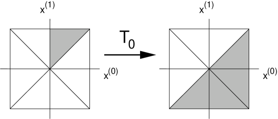
Figure 1: Transformation properties of the uncoupled tent maps (1). A simplex and its image is indicated.

The grammar is trivial in the sense that all symbol sequences consisting of pairs $(\sigma^{(0)},\sigma^{(1)})$ are permitted by the dynamics.

We are now going to introduce an interaction in such a way that the map remains piecewise linear on a suitable Markov partition and hence will allow for an analytical and elementary treatment. The strategy consists in fixing a suitable Markov partition, and then constructing the corresponding analytical form of the mapping. We start from the Markov partition of the uncoupled system and deform the partition appropriately (cf. fig.2). Consider a fixed set of the partition we intend to construct. On this set the two–dimensional map has to be affine. A general two–dimensional affine mapping has six adjustable parameters. Therefore by fixing three points in phase space and their images the affine mapping is determined uniquely. For that reason we cannot stick to the cubes, which constitute a Markov partition of the uncoupled system, but have to trace back to triangles, i.e. two–dimensional simplices. In fact, specifying a simplex and an image simplex fixes uniquely an affine transformation, which maps the former set onto the latter one. Therefore one introduces an interaction between the two tent maps, if one deforms the simplices in the Markov partition but requires that the images of these simplices coincide with the image simplices of the uncoupled case (cf. fig.2).

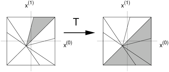
Figure 2: Simplices of the Markov partition of two coupled maps obtained by a deformation of the uncoupled case. The shaded area indicates a simplex and its image.

However the deformation cannot be performed arbitrarily, since the image of each simplex has to consist of a union of simplices in order to guarantee the Markov property. Hence vertices on the boundary of phase space have to stay on the boundary, and the vertex on the diagonal has to stay on the diagonal. This simple geometrical prescription constitutes the basic idea for the construction of the coupled map lattice. In what follows a suitable notation will be introduced, in order to present the analytical expressions for the map and the associated partition function. The approach will be held general enough to capture the case of arbitrary dimension too.

To label the simplices again we start from the uncoupled case. The simplices are obtained by dividing each square (2) into two simplices as indicated in fig.1. Each simplex has three vertices, the first being given by a ”corner” of the phase space $(\sigma^{(0)},\sigma^{(1)})$, the second being given by the intersection of the boundary and the coordinate axis, and the last one is located at the centre $(0,0)$. Corresponding to these vertices the following symbol is assigned to the two resulting simplices

$$\{(\sigma^{(0)},\sigma^{(1)}),(0,\sigma^{(1)}),(0,0)\} \leftrightarrow [(\sigma^{(0)},\sigma^{(1)});I]$$

$$\{(\sigma^{(0)},\sigma^{(1)}),(\sigma^{(0)},0),(0,0)\} \leftrightarrow [(\sigma^{(0)},\sigma^{(1)});Q]\quad.$$ (3)

Alternatively this convention corresponds to the notation

$$[(\sigma^{(0)},\sigma^{(1)});P]:=\{(x^{(0)},x^{(1)})\,|\,0\leq\sigma^{P(0)}x^{P(0)}\leq\sigma^{P(1)}x^{P(1)}\leq 1\}\quad,$$ (4)

if $P$ denotes a permutation which is either $Q$, the transposition of the two numbers $0,1$ or $I$, the identity permutation. Within this notation the uncoupled map $T_{0}$ induces the following transitions, i.e. the grammar of the system

$$[(\sigma^{(0)},\sigma^{(1)});I] \rightarrow [(1,1);Q]\cup[(1,-1);Q]\cup[(1,-1);I]\cup[(-1,-1);I]$$

$$\,[(\sigma^{(0)},\sigma^{(1)});Q] \rightarrow [(1,1);I]\cup[(-1,1);Q]\cup[(-1,1);I]\cup[(-1,-1);Q]\quad.$$ (5)

As already mentioned the interaction between the tent maps is introduced, by shifting the vertices $(\pm 1,0)$ and $(0,\pm 1)$ along the boundary an amount, which we denote by $t_{(\pm 1,0)}$ and $t_{(0,\pm 1)}$ respectively. The shifted vertices read $(\pm 1,t_{(\pm 1,0)})$ and $(t_{(0,\pm 1)},\pm 1)$. In the same way the vertex on the diagonal $(0,0)$ is shifted to $(t_{(0,0)},t_{(0,0)})$. The deformed simplex $[(\sigma^{(0)},\sigma^{(1)});P]$, to which we assign the same label, possesses the vertices

$$[(\sigma^{(0)},\sigma^{(1)}),P]\leftrightarrow\left\{\begin{array}[]{ll}\{(\sigma^{(0)},\sigma^{(1)}),(t_{(0,\sigma^{(1)})},\sigma^{(1)}),(t_{(0,0)},t_{(0,0)})\}&P=I\\ \{(\sigma^{(0)},\sigma^{(1)}),(\sigma^{(0)},t_{(\sigma^{(0)},0)}),(t_{(0,0)},t_{(0,0)})\}&P=Q\end{array}\right.\quad.$$ (6)

The grammar (2) and the condition that the map acts linearly on the simplices, define the dynamical system completely. Within this setting the numbers $t_{(\sigma,\sigma^{\prime})}$ act as parameters for the map $T$.

It is now possible to evaluate the partition function corresponding to the topological pressure. For that purpose we need the local expansion rate, i.e. the Jacobian. The latter is easily obtained from the ratio of the volume of a simplex and the volume of its image. Hence there is no need to write down the closed analytical formula for the coupled system at the moment. If one introduces the notation $\underline{\sigma}=(\sigma^{(0)},\sigma^{(1)})$ and

$$\underline{\sigma}^{\{0\}}:=(0,\sigma^{(1)}),\quad\underline{\sigma}^{\{1\}}:=(\sigma^{(0)},0),\quad\underline{\sigma}^{\{0,1\}}:=(0,0)$$ (7)

then the volume of the simplex (6) is given by

$$\mbox{Vol}[(\sigma^{(0)},\sigma^{(1)}),P] = \frac{1}{2}\left|\sigma^{P(0)}-t_{\underline{\sigma}^{P\{0\}}}\right|\left|\sigma^{P(1)}-t_{\underline{\sigma}^{P\{0,1\}}}\right|$$ (8)

$$= \frac{1}{2}\left(1-\sigma^{P(0)}t_{\underline{\sigma}^{P\{0\}}}\right)\left(1-\sigma^{P(1)}t_{\underline{\sigma}^{P\{0,1\}}}\right)\quad.$$

Since the volume of the image is always given by $2^{2}/2$ (cf. fig.2) one obtains for the Jacobian the expression

$$\left|\det DT\right|_{[\underline{\sigma},P]}=2^{2}\left(1-\sigma^{P(0)}t_{\underline{\sigma}^{P\{0\}}}\right)^{-1}\left(1-\sigma^{P(1)}t_{\underline{\sigma}^{P\{0,1\}}}\right)^{-1}\quad.$$ (9)

Performing the summation over all $n$–periodic symbol sequences $[\underline{\sigma}_{0};P_{0}],\ldots,$ $[\underline{\sigma}_{n-1};P_{n-1}],[\underline{\sigma}_{0};P_{0}],\ldots$ that are permitted by the grammar (2) yields for the partition sum corresponding to the local expansion rate the expression

$$Z_{n}(\beta)=\sum^{\prime}\prod_{k=0}^{n-1}2^{-2\beta}\left(1-\sigma_{k}^{P_{k}(0)}t_{\underline{\sigma}_{k}^{P_{k}\{0\}}}\right)^{\beta}\left(1-\sigma_{k}^{P_{k}(1)}t_{\underline{\sigma}_{k}^{P_{k}\{0,1\}}}\right)^{\beta}\quad.$$ (10)

The summation in eq.(10) involves both a summation over symbol patterns $\{\sigma_{k}^{(\nu)}\}$ and over sequences of permutations $P_{k}$ which are related by the grammar. In order to read off the spin Hamiltonian from eq.(10) the summation with respect to the permutation sequences has to be performed. But as indicated in appendix A this sequence is almost uniquely determined by the symbol pattern, if surface terms are discarded. Hence expression (10) may be understood as a sum over all periodic symbol patterns $\{\sigma_{k}^{(\nu)}\}$, with the sequence of permutations being determined by this pattern according to the grammar (2). Summarising, eq.(10) represents the partition sum of two coupled spin chains with the interaction being mediated by the deformation parameters $t$, i.e. by the coupling in the dynamical system. No phase transition occurs of course, since no long range interactions are involved.

3 Ising type transition in a globally coupled model

The considerations of the preceding section will be carried over to the case of $L$ coupled maps, where $L$ may be understood as the extension in the ”spatial” direction of the dynamical system.

We start again from $L$ independent tent maps. Let $\underline{x}=(x^{(0)},\ldots,x^{(L-1)})$ specify the state of the system in the phase space $[-1,1]^{L}$. Each cube of the Markov partition, as usual labelled by $\underline{\sigma}\in\{-1,1\}^{L}$, is divided into $L!$ simplices according to (cf. eq.(4))

$$[\underline{\sigma};P]:=\{\underline{x}\,|\,0\leq\sigma^{P(0)}x^{P(0)}\leq\ldots\leq\sigma^{P(L-1)}x^{P(L-1)}\leq 1\}\quad,$$ (11)

where $P$ denotes a permutation of the $L$ numbers $0,\ldots,L-1$. The vertices of this simplex are given by

$$\underline{\sigma},\underline{\sigma}^{P\{0\}},\ldots,\underline{\sigma}^{P\{0,\ldots,L-1\}}\quad.$$ (12)

Here $\underline{\sigma}^{P\{0,\ldots,\nu\}}$ denotes the phase space point which is obtained by replacing the entries at positions $P(0),\ldots,P(\nu)$ in the symbol sequence $\underline{\sigma}$ with zero. Uncoupled tent maps have the property, that the image $T_{0}(\underline{\sigma}^{P\{0,\ldots,\nu\}})$ of a vertex is obtained, if each coordinate with value $\pm 1$ is replaced by $-1$, and each coordinate with value $0$ is replaced by $+1$. Using this rule the grammar corresponding to the partition (11) can be constructed, but we will not need these expressions in what follows.

The interaction among the maps is introduced by deforming the simplices, i. e. by shifting the coordinates of the vertices (12) which are zero by a constant amount. The shifted vertex is generated from $\underline{\sigma}^{P\{0,\ldots,\nu\}}$ by replacing every zero in the sequence by the same constant value $t_{\underline{\sigma}^{P\{0,\ldots,\nu\}}}$, which of course is smaller than $1$ in modulus (cf. eqs.(2) and (6)). The shift may differ from vertex to vertex as indicated by the subscript. For the shifted vertex the notation $\underline{\tau}_{\underline{\sigma}^{P\{0,\ldots,\nu\}}}$ is introduced. The construction of the coupled map lattice is completed by the condition that the image of the vertex is given by the image of the corresponding vertex of the uncoupled system $T(\underline{\tau}_{\underline{\sigma}^{P\{0,\ldots,\nu\}}})=T_{0}(\underline{\sigma}^{P\{0,\ldots,\nu\}})$. The last condition guarantees that the image of each simplex is given by a union of simplices like in the uncoupled case. Since a closed analytical formula of the coupled map lattice $T$ will be of no use for us, I refrain from writing down such an expression. However for numerical purposes appendix B contains a simple recursive algorithm to evaluate $T$.

In order to determine the Jacobian one needs the volume of the deformed simplices. The latter follows immediately from the vertices described above as

$$\mbox{Vol}[\underline{\sigma};P]=\frac{1}{L!}\prod_{\nu=0}^{L-1}\left(1-\sigma^{P(\nu)}t_{\underline{\sigma}^{P\{0,\ldots,\nu\}}}\right)\quad.$$ (13)

Since the image of each simplex has the volume $2^{L}/L!$ the Jacobian reads

$$\left|\det DT\right|_{[\underline{\sigma};P]}=2^{L}\prod_{\nu=0}^{L-1}\left(1-\sigma^{P(\nu)}t_{\underline{\sigma}^{P\{0,\ldots,\nu\}}}\right)^{-1}\quad.$$ (14)

Hence we obtain for the partition sum

$$Z_{n}(\beta)=\sum^{\prime}\prod_{k=0}^{n-1}2^{-L\beta}\prod_{\nu=0}^{L-1}\left(1-\sigma_{k}^{P_{k}(\nu)}t_{\underline{\sigma}_{k}^{P_{k}\{0,\ldots,\nu\}}}\right)^{\beta}\quad,$$ (15)

where again the summation has to be performed with respect to all $n$–periodic accessible symbol sequences $[\underline{\sigma}_{0};P_{0}],\ldots,[\underline{\sigma}_{n-1};P_{0}],[\underline{\sigma}_{0};P_{0}],\ldots$. As already indicated in the preceding section the permutation sequence $P_{k}$ is (almost) uniquely determined by the two–dimensional symbol pattern $\{\sigma_{k}^{(\nu)}\}$. Hence we may alternatively perform the summation with respect to all the spin variables, with the permutations being determined by the spin pattern. Then the corresponding Hamiltonian of the two–dimensional spin lattice can be read off from eq.(15) directly.

The structure of the Hamiltonian is however a little bit hidden since the permutations depend on the spin variables. To simplify the subsequent considerations we will refer in what follows to a special choice which corresponds to a globally coupled system, so that the permutations drop from the formulas. Let us choose the deformations in such a way, that on the one hand no interaction in the index $k$, i.e. in the direction of time occurs, and on the other hand a global interaction between the spins in the index $\nu$, i.e. an interaction in the spatial direction is realised. Then we are left with simple mean field Ising chains.

$$\prod_{\nu=0}^{L-1}\left(1-\sigma^{P(\nu)}t_{\underline{\sigma}^{P\{0,\ldots,\nu\}}}\right)^{\beta}=\exp\left(\beta H\sum_{\nu=0}^{L-1}\sigma^{(\nu)}+\beta\frac{J}{L}\sum_{\nu,\mu=0}^{L-1}\sigma^{(\nu)}\sigma^{(\mu)}+\beta E_{0}\right)$$ (16)

Confer appendix C for the corresponding explicit construction, which determines the deformation parameters $t_{\underline{\sigma}^{P\{0,\ldots,\nu\}}}$ in terms of $H$ and $J$ and the normalisation constant $E_{0}$. Roughly speaking the parameter $H$, corresponding to the magnetic field in the spin system, describes the deviation of the map lattice from an inversion symmetric case, whereas the spin interaction $J$ mediates the spatial coupling among the maps. Inspecting eqs.(15) and (16), the Hamiltonian of the full map lattice consists of non interacting spin chains. Since the interaction within a chain has infinite range a phase transition occurs at $\beta H=0$, $\beta J=1/2$ if the thermodynamic limit $L\rightarrow\infty$ has been performed. Hence our coupled map lattice displays a bifurcation, which is intimately related to the limit of large system size. Of course the model allows for an analytical calculation of those quantities, which are determined by the spin pattern, since the partition sum can be evaluated in the thermodynamic limit.

Let us supplement the analytical results with numerical simulations of the full map lattice (cf. appendix B and C for the numerical algorithm). Keep in mind however that the usual long time average, which will be denoted by $\langle\ldots\rangle$ in the sequel corresponds to the choice $\beta=1$ in the context of dynamical systems. Obvious global quantities are given by the spatially averaged symbol sequence and its square

$$\langle S\rangle:=\left\langle\frac{1}{L}\sum_{\nu=0}^{L-1}\sigma^{(\nu)}\right\rangle,\qquad\langle S^{2}\rangle:=\left\langle\left(\frac{1}{L}\sum_{\nu=0}^{L-1}\sigma^{(\nu)}\right)^{2}\right\rangle\quad.$$ (17)

The dependence of these averages on $H$ and $J$ is displayed in fig.3. The well known behaviour of the Ising mean field model is reproduced, but of course the results have been obtained here from the dynamics of the map lattice.

Figure 3: Dependence of the spatially averaged symbol and its square on $H$ and $J$ for system size $L=256$ and $L=128$. The time average has been performed using a spatial uniformly distributed initial condition and $2000$ iteration steps, after discarding a transient of length $200$.

One should however keep in mind that from the point of view of the dynamical system the quantities (17) look a little bit artificial and the actual interpretation of the dependence on the system parameters is difficult. Nevertheless the main feature, i. e. the second order phase transition clearly shows up at $H=0$, $J=1/2$, but finite size effects are superimposed.

In order to demonstrate the influence of the system size on the transition more clearly, consider the zero field dependence of $\langle S^{2}\rangle$ on the interaction strength for different system size (fig.4).

Figure 4: Dependence of $\langle S^{2}\rangle$ on the interaction $J$ for zero field $H=0$ and different system sizes (symbols). The solid line displays the analytical result in the thermodynamic limit $L\rightarrow\infty$.

Since the phase transition sharpens if the thermodynamic limit is approached, it is obvious that the transition in the dynamical system is intimately related to the thermodynamic limit. Hence it is a characteristic feature of the high–dimensional dynamical system.

Finally, let us have a look at the space time evolution in symbol space as well as in phase space. Consider first the evolution in an inversion symmetric situation, i.e. $H=0.0$ (cf. fig. 5).

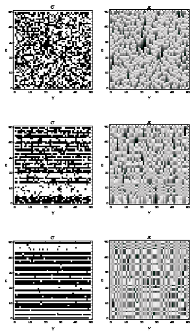
Figure 5: Space time evolution of the symbols $\sigma_{k}^{(\nu)}$ and of the phase space coordinate $x_{k}^{(\nu)}$ for a system of size $L=256$, field $H=0.0$, and coupling strengths increasing from above to below $J=0.2,0.6,1.0$. Black/white pixels correspond to the values $\sigma=-1/+1$ and dark/light pixels to phase space coordinates close to $x=-1/+1$.

Below the transition point, i. e. for weak coupling, a rather irregular state is observed. It corresponds to the space time chaotic regime mentioned in the introduction. Slightly above the transition point long range order develops, but a lot of ”defects” are superimposed. The synchronisation becomes more perfect, if the coupling is further strengthened. Of course both phases are mixed, since no symmetry breaking field is present. With a symmetry breaking field the weak coupling regime behaves very similar to the zero field case (c.f. fig.6).

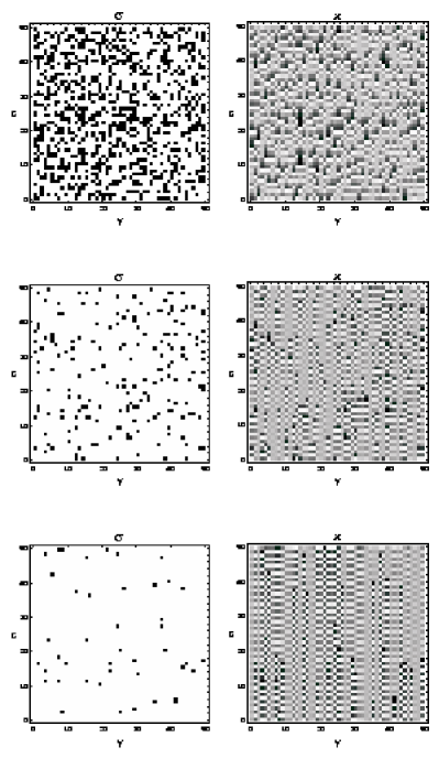
Figure 6: Space time evolution of the symbols $\sigma_{k}^{(\nu)}$ and of the phase space coordinate $x_{k}^{(\nu)}$ for a system of size $L=256$, field $H=0.2$, and coupling strengths increasing from above to below $J=0.2,0.6,1.0$. Black/white pixels correspond to the values $\sigma=-1/+1$ and dark/light pixels to phase space coordinates close to $x=-1/+1$.

But above the transition point one phase is dominant and a pure state develops if the coupling is increased. In summary, the phase transition shows up in the symbol representation as well as in the phase space coordinates, where apparently two different kinds of motion occur.

4 Conclusion

A class of piecewise linear coupled map lattices has been investigated which allows for an analytical approach. The key point of the construction consists in fixing a Markov partition in terms of simplices, imposing a grammar, and requiring the map to be linear on this partition. Such an approach allows for an elementary and analytical construction of the corresponding spin Hamiltonian. Phase transitions are possible at finite coupling in the limit of large system size, although the model is locally expanding and has the Markov property.

The proposed construction may be understood as the natural extension of piecewise linear one–dimensional maps to more than one dimension. In fact, by a refinement of the partition a large class of functions, at least in finite dimensions, can be approximated, as stated by the simplicial approximation theorem. Furthermore, piecewise linear one–dimensional maps are able to approximate dynamical features of low–dimensional chaos, as stated by the Ulam conjecture [18]. Similar properties might hold also for simplicial mappings in connection with high–dimensional dynamics, but further clarification is certainly needed.

The explicit evaluation of a phase transition has been performed for a global coupling only. Although globally coupled systems are interesting in itself I have dealt with a globally coupled system for reasons of simplicity, since otherwise the exact computation of the phase transition may become much more involved. I believe that the principal aspects of this paper do not depend on this choice of coupling. Indeed an interaction in the time direction of the spin system may be introduced by tracing back to finer partitions, and a spatial short range coupling may be realised. Hence it seems possible to construct a model along these lines which is in some sense closer to a nearest neighbour coupled Ising model in two dimensions, i. e. a model with short range interactions in each direction but admitting a phase transition in the thermodynamic limit. Since the objective of the present publication was on the principal aspect I leave this problem for future work.

In the treatment I have adopted a physicists approach, by considering systems of arbitrary but finite size and performing the thermodynamic limit at the end of the calculation. Therefore it is not easy to decide rigorously whether the dynamical system, being defined by a geometrical construction, tends to a mathematically well defined limit. Nevertheless the discussion of the example supports such a conjecture. Then the phase transition like behaviour in the finite model should be related to a transient dynamics whose duration increases with the system size. Such an analysis, which is of course desirable for a deeper understanding of the transition has not been accomplished yet.

Models of the type investigated here, i. e. models with a large number of degrees of freedom showing a phase transition and allowing for an elementary analytical approach, may be helpful to understand several features of high–dimensional chaotic dynamics. Although the grammar, i. e. the structure of space time periodic orbits was fixed by hand, it is also possible to investigate the influence of pruning, by considering increasingly finer Markov partitions. These properties together with an analytical accessible system may have an impact on the understanding of expansions in terms of space time periodic orbits, which have recently attracted some interest.

Appendix A Two coupled maps

In order to simplify our computations and not hide the main arguments behind extensive computations let us specialise to the case $t_{(0,\sigma)}=t_{(\sigma,0)}=-\sigma\tanh J$, $t_{(0,0)}=0$. I think it will become evident that this choice does not influence the generality of the arguments.

The partition sum (10) is taken with respect to all $n$–periodic sequences $([\underline{\sigma}_{k};P_{k}])$. Consider first those patterns which obey $\sigma_{k}^{(0)}\neq\sigma_{k}^{(1)}$ for some index $k\in[0,n-1]$. Since the symbols $(\sigma^{(0)},\sigma^{(1)})$, that means the sets $[\underline{\sigma};I]\cup[\underline{\sigma};Q]$, already determine a Markov partition, the pattern $\{\sigma_{k}^{(\nu)}\}$ specifies a phase space point, which in our case is a period–$n$ orbit. But this orbit does not hit a boundary of the simplices and especially not the diagonal of the phase space, since at least one pair of symbols has different entries. The validity of this statement is obvious for the case of noninteracting maps. It carries over to the general case, since the deformation of the simplices does not destroy topological properties in the phase space. Hence the sequence of permutations $P_{k}^{(\nu)}$ is determined uniquely by the periodic orbit, that means by the pattern of symbols $\{\sigma_{k}^{(\nu)}\}$.

Consider instead $\sigma_{k}^{(0)}=\sigma_{k}^{(1)}$ for all $k$, i.e. a synchronised orbit. Then the corresponding phase space point is located on the diagonal, i. e. on the boundary of the simplices. From the grammar (2) we have that the predecessor $P_{k}$ of a permutation $P_{k+1}$ changes according to the symbol $\sigma_{k+1}^{(0/1)}$ and obeys

$$P_{k}=P_{k+1}\mbox{ if }\sigma_{k+1}^{(0/1)}=-1\qquad P_{k}=QP_{k+1}\mbox{ if }\sigma_{k+1}^{(0/1)}=1\quad.$$ (18)

The condition that the sequence $P_{k}$ is $n$–periodic, $P_{0}=P_{n}$, requires that the finite sequence $(\sigma_{0}^{(0/1)},\ldots,\sigma_{n-1}^{(0/1)})$ contains an even number of symbols $+1$. Furthermore there exist two corresponding permutation sequences according to eq.(18) and the choice $P_{0}=I,Q$.

Then the partition sum (10) splits into two parts, one part containing the summation over non synchronised symbol patterns, and the second part containing the summation over synchronised symbol patterns with an even number of $+1$ symbols and two complementary permutation sequences. If we supplement the first part with the missing synchronised symbol sequences then eq.(10) reads

$$Z_{n}(\beta) = \sum_{\sigma_{k}^{(0)},\sigma_{k}^{(1)}}\prod_{k=0}^{n-1}2^{-2\beta}\left(1-\sigma_{k}^{P_{k}(0)}t_{\underline{\sigma}_{k}^{P_{k}\{0\}}}\right)^{\beta}\left(1-\sigma_{k}^{P_{k}(1)}t_{\underline{\sigma}_{k}^{P_{k}\{0,1\}}}\right)^{\beta}$$ (19)

$$+ \sum_{\sigma_{k}^{(0)}=\sigma_{k}^{(1)},even}\prod_{k=0}^{n-1}2^{-2\beta}\left(1-\sigma_{k}^{P_{k}(0)}t_{\underline{\sigma}_{k}^{P_{k}\{0\}}}\right)^{\beta}\left(1-\sigma_{k}^{P_{k}(1)}t_{\underline{\sigma}_{k}^{P_{k}\{0,1\}}}\right)^{\beta}$$

$$- \sum_{\sigma_{k}^{(0)}=\sigma_{k}^{(1)},odd}\prod_{k=0}^{n-1}2^{-2\beta}\left(1-\sigma_{k}^{P_{k}(0)}t_{\underline{\sigma}_{k}^{P_{k}\{0\}}}\right)^{\beta}\left(1-\sigma_{k}^{P_{k}(1)}t_{\underline{\sigma}_{k}^{P_{k}\{0,1\}}}\right)^{\beta}$$

where the index even/odd means, that the summation is performed with respect to sequences containing an even/odd number of $+1$ symbols. Now in each sum the sequence of permutations is uniquely determined by the symbol pattern $\{\sigma_{k}^{(\nu)}\}$. By our choice of deformations the relation

$$\left(1-\sigma_{k}^{P_{k}(0)}t_{\underline{\sigma}_{k}^{P_{k}\{0\}}}\right)^{\beta}\left(1-\sigma_{k}^{P_{k}(1)}t_{\underline{\sigma}_{k}^{P_{k}\{0,1\}}}\right)^{\beta}=\left(1+\sigma_{k}^{(0)}\sigma_{k}^{(1)}\tanh J\right)^{\beta}$$ (20)

holds, and it is exactly this property which simplifies the subsequent considerations. Furthermore we perform in the second and third sum of eq.(19) an unconstrained summation over $\sigma_{k}$, $0\leq k\leq n-2$, choosing $\sigma_{n-1}$ in such a way that the constraint of an even or odd number of $+1$ values is guaranteed. Then we get

$$Z_{n}(\beta) = \sum_{\sigma_{k}^{(0)},\sigma_{k}^{(1)}}\prod_{k=0}^{n-1}2^{-2\beta}\left(1+\sigma_{k}^{(0)}\sigma_{k}^{(1)}\tanh J\right)^{\beta}$$

$$+ \sum_{\sigma_{0},\ldots,\sigma_{n-2}}\prod_{k=0}^{n-2}2^{-2\beta}\left(1+\tanh J\right)^{\beta}\left\{\left(1+\tanh J\right)^{\beta}-\left(1+\tanh J\right)^{\beta}\right\}\quad.$$

The second contribution vanishes identically. Now the Hamiltonian can be read off directly from the partition sum

$$-\beta{\cal H}=-\beta\sum_{k=0}^{n-1}\left(-J\sigma_{k}^{(0)}\sigma_{k}^{(1)}+\ln\cosh J+\ln 4\right)\quad.$$ (22)

We end up with a simple pair interaction in the ”spatial” direction and no interaction in the ”time” direction.

Appendix B $L$–dimensional simplicial mapping

For a given set of deformation parameters $t_{\underline{\sigma}^{P\{0,\ldots,\nu\}}}$ a recursive algorithm will be developed, which allows for the calculation of the image point $T(\underline{x})$. Let us assume that $\underline{x}$ is contained in the interior of a simplex, which from the point of view of a numerical evaluation causes no restriction for the continuous mapping $T$. Since the simplices are deformed, it is a nontrivial task to determine the simplex, that contains a given phase space point $\underline{x}$. However using the fact that simplices are convex, a sequence of projections is adopted to determine the corresponding set, the simplicial coordinates and hence the image point (cf. fig.7).

Figure 7: Diagrammatic view of the recursive projections onto lower–dimensional faces of the simplex, which are used to determine the simplex containing the phase space point $\underline{x}$. The box indicates a quadrant $[0,1]^{3}$, $\underline{\tau}_{k}$ denote the vertices of the simplex, and $\underline{x}_{[k]}$ the sequence of the projected points.

Let $\underline{x}_{[0]}=\underline{x}$ denote the phase space point, and $\underline{\tau}_{0}:=\underline{\tau}_{\underline{\sigma}^{P\{0,\ldots,L-1\}}}=(t_{0},t_{0},\ldots,t_{0})$ with $t_{0}:=t_{\underline{\sigma}^{P\{0,\ldots,L-1\}}}=t_{(0,\ldots,0)}$ the central vertex in the cube $[-1,1]^{L}$. By our construction this vertex is common to all the simplices and hence is a vertex of the simplex which contains the phase space point $\underline{x}$. Consider the semi–infinite ray emanating from $\underline{\tau}_{0}$ through $\underline{x}_{[0]}$. It intersects the surface of the cube $[-1,1]^{L}$ at a point denoted by $\underline{x}_{[1]}$

$$\underline{x}_{[1]}=s_{0}\underline{x}_{[0]}+(1-s_{0})\underline{\tau}_{0}\quad.$$ (23)

Here $s_{0}$ denotes the number which makes the expression

$$s_{0}:=\frac{1}{|x^{(k_{0})}_{[0]}-t_{0}|}-\frac{t_{0}}{x^{(k_{0})}_{[0]}-t_{0}}\rightarrow{\min}$$ (24)

minimal among all components $k$. The component $k_{0}$ for which the minimum is attained determines the surface of the cube where the intersection occurs by the condition $x^{(k_{0})}=\sigma^{(k_{0})}$, with $\sigma^{(k_{0})}$ being given by

$$\sigma^{(k_{0})}=\mbox{sign}(x^{(k_{0})}_{[0]}-t_{0})\quad.$$ (25)

That surface contains one face of the simplex we are looking for. If we define $P(L-1):=k_{0}$, then the central vertex within this surface reads $\underline{\tau}_{1}:=\underline{\tau}_{\underline{\sigma}^{P\{0,\ldots,L-2\}}}$, and it leads to the second vertex of the simplex we are looking for. Now one repeats the same reasoning using the points $\underline{x}_{[1]}$ and $\underline{\tau}_{1}$, but with the dimension of the problem being reduced by one.

Hence one continues by induction. Determine $k_{\mu}\not\in\{P(L-1),\ldots,P(L-\mu)\}$ among those components, which have not been fixed yet, such that

$$s_{\mu}:=\frac{1}{|x^{(k_{\mu})}_{[\mu]}-t_{\mu}|}-\frac{t_{\mu}}{x^{(k_{\mu})}_{[\mu]}-t_{\mu}}\rightarrow{\min}$$ (26)

is minimal. Here $t_{\mu}:=t_{\underline{\sigma}^{P\{0,\ldots,L-1-\mu\}}}$. Then

$$\sigma^{(k_{\mu})}:=\mbox{sign}(x^{(k_{\mu})}_{[\mu]}-t_{\mu})$$ (27)

and $P(L-1-\mu):=k_{\mu}$ determine the next components of the symbol sequence and the permutation respectively.

$$\underline{x}_{[\mu+1]}=s_{\mu}\underline{x}_{[\mu]}+(1-s_{\mu})\underline{\tau}_{\mu}$$ (28)

yields the new intersection point, using the abbreviation $\underline{\tau}_{\mu}=\underline{\tau}_{\underline{\sigma}^{P\{0,\ldots,L-1-\mu\}}}$. This iteration terminates exactly after $L$ steps, since we end up with a corner point of the cube $[-1,1]^{L}$. It yields the simplex $[\underline{\sigma};P]$ which contains the point $\underline{x}$.

In addition we can read off the simplicial coordinates $0\leq\lambda_{\mu}\leq 1$ which are defined by

$$\underline{x}=\sum_{\mu=0}^{L}\lambda_{\mu}\underline{\tau}_{\mu},\qquad\sum_{\mu=0}^{L}\lambda_{\mu}=1\quad.$$ (29)

These coordinates are particularly useful for the evaluation of the image point $T(\underline{x})$. Recalling that the map $T$ is linear on the simplex, and that the images of the vertices $\underline{\tau}_{\mu}$ are obtained, by replacing the components with values $\pm 1$ by $-1$ and the components with values $t_{\mu}$ by $+1$, we get

$$\left(T(\underline{x})\right)^{P(\nu)} = \sum_{\mu=0}^{\nu}\lambda_{\mu}\left(T(\underline{\tau}_{\mu})\right)^{P(\nu)}+\sum_{\mu=\nu+1}^{L}\lambda_{\mu}\left(T(\underline{\tau}_{\mu})\right)^{P(\nu)}=\sum_{\mu=0}^{\nu}\lambda_{\mu}-\sum_{\mu=\nu+1}^{L}\lambda_{\mu}$$ (30)

$$= -1+2\sum_{\mu=0}^{\nu}\lambda_{\mu}\quad.$$

Furthermore we can express the simplicial coordinates in terms of the quantities (26), which have already been determined in the course of the recursion. As we prove at the end of this appendix

$$\sum_{\mu=0}^{\nu}\lambda_{\mu}=1-\left(\prod_{\mu=0}^{\nu}s_{\mu}\right)^{-1}$$ (31)

holds for $0\leq\nu\leq L-1$. Hence the simple recursion scheme described above together with eqs.(30) and (31) complete the algorithm for the numerical evaluation of the map lattice.

We are left with verifying eq.(31). Again an induction will be used. First the component $P(L-1)$ of eq.(29) yields

$$x^{P(L-1)}=\lambda_{0}t_{0}+(1-\lambda_{0})\sigma^{P(L-1)}\quad.$$ (32)

Then using the definition (25) one obtains

$$\frac{1}{1-\lambda_{0}}=\frac{1}{|x_{[0]}^{P(L-1)}-t_{0}|}-\frac{t_{0}}{x_{[0]}^{P(L-1)}-t_{0}}\quad,$$ (33)

which by virtue of eq.(24) leads to the result (31) for $\nu=0$. Suppose that (31) holds for $\nu\leq\rho$. Evaluation of eq.(29) for the component $P(L-\rho-2)$ yields

$$x^{P(L-\rho-2)}_{[0]}=\lambda_{0}t_{0}+\ldots+\lambda_{\rho+1}t_{\rho+1}+(1-\lambda_{0}-\ldots-\lambda_{\rho+1})\sigma^{P(L-\rho-2)}\quad.$$ (34)

On the other hand, we obtain from the recursion relation (28)

$$x_{[\rho+1]}^{P(L-\rho-2)}-t_{\rho+1} = (s_{0}\ldots s_{\rho})\left(x_{[0]}^{P(L-\rho-2)}+\frac{(1-s_{0})t_{0}}{s_{0}}+\frac{(1-s_{1})t_{1}}{s_{0}s_{1}}+\ldots\right.$$ (35)

$$+ \left.\frac{(1-s_{\rho})t_{\rho}}{s_{0}\ldots s_{\rho}}-\frac{t_{\rho+1}}{s_{0}\ldots s_{\rho}}\right)\quad.$$

If one now inserts eq.(34) into eq.(35) and repeatedly uses eq.(31) for $\nu\leq\rho$ one gets

$$x_{[\rho+1]}^{P(L-\rho-2)}-t_{\rho+1}$$ (36)

$$= (s_{0}\ldots s_{\rho})\left((1-\lambda_{0}-\ldots-\lambda_{\rho+1})\sigma^{P(L-\rho-2)}+\lambda_{\rho+1}t_{\rho+1}-\frac{t_{\rho+1}}{s_{0}\ldots s_{\rho}}\right)$$

$$= (1-\lambda_{0}-\ldots-\lambda_{\rho+1})(s_{0}\ldots s_{\rho})\left(\sigma^{P(L-\rho-2)}-t_{\rho+1}\right)\quad.$$

But then from the definition (27) we have

$$\frac{1}{1-\lambda_{0}-\ldots\lambda_{\rho+1}}=(s_{0}\ldots s_{\rho})\left(\frac{1}{|x_{[\rho+1]}^{P(L-\rho-2)}-t_{\rho+1}|}-\frac{t_{\rho+1}}{x_{[\rho+1]}^{P(L-\rho-2)}-t_{\rho+1}}\right)$$ (37)

and the result follows from the definition (26).

Appendix C Spatial mean field coupling

Using the abbreviation

$$S_{\nu}:=\sum_{\mu=\nu+1}^{L-1}\sigma^{(\mu)}$$ (38)

a sequence of functions $g_{\nu}(S_{\nu})$ will be constructed which obeys

$$\sum_{\nu=0}^{L-1}\sigma^{(\nu)}\left(\frac{2J}{L}S_{\nu}+H\right)+J+E_{0}=\sum_{\nu=0}^{L-1}\ln\left(1-\sigma^{(\nu)}\tanh g_{\nu}(S_{\nu})\right)$$ (39)

with a constant $E_{0}$ being independent of the spin variables. Since the left hand side is invariant with respect to a permutation of the spin numbers the result (16) follows then immediately if one defines

$$t_{\underline{\sigma}^{P\{0,\ldots,\nu\}}}:=\tanh g_{\nu}\left(\sum_{\mu\not\in P\{0,\ldots,\nu\}}\sigma^{(\mu)}\right)\quad.$$ (40)

Applying the trivial identity

$$f(\sigma)=\sigma[f(+1)-f(-1)]/2+[f(+1)+f(-1)]/2$$ (41)

one obtains

$$\ln\left(1-\sigma^{(\nu)}\tanh g_{\nu}(S_{\nu})\right)=-\sigma^{(\nu)}g_{\nu}(S_{\nu})-h_{\nu}(S_{\nu})$$ (42)

if the abbreviation $h_{\nu}(x):=\ln\cosh g_{\nu}(x)$ is introduced. Observing $S_{\nu}=\sigma^{(\nu+1)}+S_{\nu+1}$ and applying eq.(41) again to the second term on the right hand side one gets

$$h_{\nu}(S_{\nu})$$

$$= \sigma^{(\nu+1)}\frac{h_{\nu}(1+S_{\nu+1})-h_{\nu}(-1+S_{\nu+1})}{2}+\frac{h_{\nu}(1+S_{\nu+1})+h_{\nu}(-1+S_{\nu+1})}{2}\quad.$$

If we repeat these steps for the last term on the right hand side and recall that by definition $S_{L-1}=0$, one ends up with

$$h_{\nu}(S_{\nu})$$ (48)

$$= \sum_{n=0}^{L-2-\nu}\sigma^{(n+\nu+1)}\frac{1}{2^{n+1}}\sum_{k=0}^{n+1}\left[\left(\begin{array}[]{c}n\\ k\end{array}\right)-\left(\begin{array}[]{c}n\\ k-1\end{array}\right)\right]h_{\nu}(n+1-2k+S_{n+1+\nu})$$

$$+ \frac{1}{2^{L-1-\nu}}\sum_{k=0}^{L-1-\nu}\left(\begin{array}[]{c}L-1-\nu\\ k\end{array}\right)h_{\nu}(L-1-\nu-2k)\quad.$$ (51)

Insert eqs.(48) and (42) into eq.(39) and equate the coefficients of $\sigma^{(\nu)}$ on both sides to obtain finally

$$\frac{2J}{L}S_{\nu}+H=-g_{\nu}(S_{\nu})-\sum_{\rho=1}^{\nu}\frac{1}{2^{\rho}}\sum_{k=0}^{\rho}\left[\left(\begin{array}[]{c}\rho-1\\ k\end{array}\right)-\left(\begin{array}[]{c}\rho-1\\ k-1\end{array}\right)\right]h_{\nu-\rho}(\rho-2k+S_{\nu})\quad.$$ (52)

This system of equations defines recursively the functions $g_{\nu}(S_{\nu})$ for increasing index $\nu$. Since the independent variable is discrete and takes only a finite number of values, the numerical evaluation is quite straightforward. It should be remarked that a simple asymptotic evaluation for large system size $L$ is possible too. Such an evaluation indicates that $g_{\nu}(S_{\nu})$ remains uniformly bounded in the limit of infinite system size.

References

- [1] M. C. Cross and P. C. Hohenberg, Pattern formation outside of equilibrium, Rev. Mod. Phys. 65, 851, 1993
- [2] K. Kaneko, Theory and applications of coupled map lattices, Wiley 1993
- [3] K. Kaneko, Pattern dynamics in spatiotemporal chaos, Physica D 34, 1, 1989
- [4] L. A. Bunimovich and Ya G. Sinai, Spacetime chaos in coupled map lattices, Nonlin. 1, 491, 1988
- [5] J. Bricmont and A. Kupiainen, Coupled analytic maps, Nonlin. 8, 379, 1995
- [6] N. Mori, T. Kobayashi, H. Hata, T. Morita, T. Horita, and H. Mori, Scaling structures and statistical mechanics of type I intermittent chaos, Prog. Theor. Phys. 81, 60, 1989
- [7] X. J. Wang, Statistical physics of temporal intermittency, Phys. Rev. A 40, 6647, 1989
- [8] W. Just and H. Fujisaka, Gibbs measures and power spectra for type I intermittent maps, Physica D 64, 98, 1993
- [9] L. A. Bunimovich, Coupled map lattices: one step forward and two steps back, Physica D 86, 248, 1995
- [10] V. L. Volevich, Kinetics of coupled map lattices, Nonlin. 4, 37, 1991
- [11] L. A. Bunimovich and E. A. Carlen, On the problem of stability in lattice dynamical systems, J. Diff. Eq. 123, 213, 1995
- [12] L. A. Bunimovich and S. Venkatagiri, Onset of chaos in coupled map lattices via the peak–crossing bifurcation, Nonlin. 9, 1281, 1996
- [13] J. Miller and D. Huse, Macroscopic equilibrium from microscopic irreversibility in a coupled–map lattice, Phys. Rev. E 48, 2528, 1993
- [14] C. Boldrighini, L. A. Bunimovich, G. Cosimi, S. Frigio, and A. Pellegrinotti, Ising–type transitions in coupled–map lattices, J. Stat. Phys. 80, 1185, 1995
- [15] K. Kaneko, Supertransients, spatiotemporal intermittency and stability of fully developed spatiotemporal chaos, Physica D 55, 368, 1990
- [16] W. Just, Globally coupled maps: phase transitions and synchronization, Physica D 81, 317, 1995
- [17] T. Yamada and H. Fujisaka, Stability theory of synchronized motion in coupled–oscillator systems III, Prog. Theor. Phys. 72, 885, 1984
- [18] M. Blank and G. Keller, Stochastic stability versus localization in one–dimensional chaotic dynamical systems, Nonlin. 10, 81, 1997