Fractal tracer distributions in turbulent field theories

Abstract

We study the motion of passive tracers in a two-dimensional turbulent velocity field generated by the Kuramoto-Sivashinsky equation. By varying the direction of the velocity-vector with respect to the field-gradient we can continuously vary the two Lyapunov exponents for the particle motion and thereby find a regime in which the particle distribution is a strange attractor. We compare the Lyapunov dimension to the information dimension of actual particle distributions and show that there is good agreement with the Kaplan-Yorke conjecture. Similar phenomena have been observed experimentally.

and

1 Introduction

The velocity field of particles confined to the surface of a fluid does not have to be incompressible even though the fluid itself is incompressible. It has correspondingly been observed experimentally [1, 2], that tracer particles moving only on the two-dimensional surface of a three-dimensional fluid can lie on a strange attractor as shown in FIG. 1. In these experiments some $50$ million floating particles were advected on the surface of the fluid, which was heavily stirred from time to time, with the stirrings done so seldom, that the fluid had time to come to rest. Pictures of the particle distributions were then examined and were found to have a well-defined fractal dimension between 1 and 2 and hence to be a strange attractor, which changed shape for each stirring. This has been explained theoretically in terms of “random maps” [3, 4], which seems appropriate for this pulsed flow. On the other hand, this phenomenon is rather general and should also occur in systems with no separation between a stirring and relaxing phase. To investigate this possibility we have looked at the advection of passive scalars in a simple turbulent field theory, the Kuramoto-Sivashinsky (KS) equation, which has been derived e.g. in the context of chemical turbulence [5] and the flow of a falling fluid film [6].

2 Advection by the 1D Kuramoto-Sivashinsky Equation

The Kuramoto-Sivashinsky equation in 1+1 dimensions is given as

$$h_{t}=-h_{xxxx}-h_{xx}+(h_{x})^{2}$$ (1)

where $h$ is a scalar field and $f_{x}\equiv\frac{\partial f}{\partial x}$. The boundary conditions are periodic on $x\in[0,L]$. The equation for the derivative $u=h_{x}$ yields

$$u_{t}=-u_{xxxx}-u_{xx}+2uu_{x}.$$ (2)

This equation has the same nonlinear term as the Navier-Stokes equations. It is thus natural to look at the field $u=h_{x}$ as a velocity field and study the motion of a passive particle with the equations of motion $\frac{dx}{dt}=ah_{x}(x,t)$, where $a$ is a real constant that gives the ratio of the time scales of the particle motion and the $h$-field. Note that the $h$-field itself is not a good choice for a velocity field, since the equation (1) is invariant under the transformation $h\rightarrow h+const$.

Such a study was carried out by Bohr and Pikovsky [7]. They examined the case $a=1$ and found the particles to diffuse anomalously, i.e., the average displacement in time goes approximately as $<x(t)^{2}>^{\frac{1}{2}}\propto t^{2/3}$, which is faster than usual diffusion. They also found, for systems seeded with several particles, that particles coalesce in time. Therefore the Lyapunov exponent for the particles is negative even though they move in a chaotic velocity field. Thus, the system exhibits Eulerian but not Lagrangian chaos.

3 Advection by the 2D Kuramoto-Sivashinsky Equation

It is trivial to generalize the Kuramoto-Sivashinsky equation (1) to two dimensions. The equation is given as

$${\partial h\over\partial t}=-{\bf\nabla}^{4}h-{\bf\nabla}^{2}h+({\bf\nabla}h)\cdot({\bf\nabla}h).$$ (3)

The $h$-field is now a function $h=h(x,y,t)$, and ${\bf\nabla}={\bf i}\frac{\partial}{\partial x}+{\bf j}\frac{\partial}{\partial y}$. For the higher order derivatives, we use the identities $\nabla^{2}=\nabla\cdot\nabla$ and $\nabla^{4}=\nabla\cdot\nabla(\nabla\cdot\nabla)$. The reason for the simplicity in the generalization is that all terms are scalar products and hence scalars. Again we assume periodic boundary conditions on $(x,y)\in[0,L]\times[0,L]$.

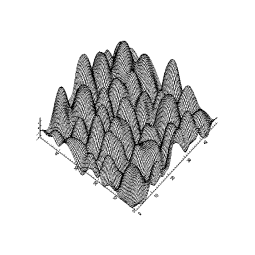
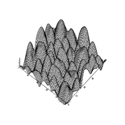
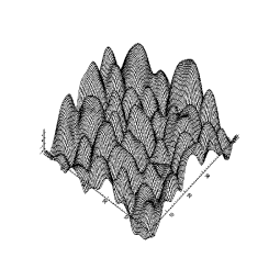
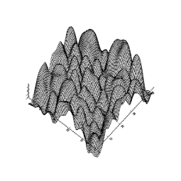
Figure 2: Solutions to the 2D Kuramoto-Sivashinsky equation at four consecutive times. Time going with $\Delta t=1$ from upper left to lower right. The system size is $50x50$.

With random initial conditions and periodic boundary conditions, the solutions look like mountain ranges: mountains (maxima) are separated from each other by valleys (minima). The valleys form a web where the mountains are isolated holes in the web. In the course of the dynamics mountains are created spontaneously or by splitting large mountains into (2,3 or 4) smaller ones - or they can disappear by being “squeezed” by neighbouring mountains. FIG. 2 shows solutions to the 2D KS-equation with $L=50$ at four consecutive time steps.

3.1 Choice of velocity field

The most obvious choice of velocity field is, as in the 1D-case, a field proportional to the gradients of the $h$-field, i.e.,

$${\bf v}_{g}=a{\bf\nabla}h$$ (4)

where the real constant $a$, as in the 1D-case, is the ratio of the time scales of the particle motion and the $h$-field. The gradient always points in the direction of the local maxima. This causes particles with different initial positions to coalesce at these maxima, similar to what is seen in the 1D-case [7]. Thus, particles moving in the gradient velocity field have both Lyapunov exponents $\lambda_{1},\lambda_{2}$ less than zero. The original field $h$ can be regarded as a velocity potential. This motion of particles is area contracting and hence dissipative. In terms of fluid dynamics, the velocity field ${\bf\nabla}h$ is compressible.

We can generalize the equations of motion (4) by a linear function of the gradient vectors. Since we want to preserve the isotropy of the KS-equation, the only possibility for the generalization is scaling and rotation. The generalized velocity field is thus constructed as a multiplication of a constant $a$, the rotation matrix ${\bf B}_{\theta}$ and the gradient vectors:

$${\bf v}=a{\bf B}_{\theta}\nabla h\quad\mbox{where}\quad{\bf B}_{\theta}=\left(\begin{array}[]{cc}\cos{\theta}&\sin{\theta}\\ -\sin{\theta}&\cos{\theta}\\ \end{array}\right)$$ (5)

Of special interest is the vector rotated $90^{\circ}$ from the gradient:

$${\bf v}_{h}=a{\bf B}_{90^{\circ}}\nabla h=\left(\begin{array}[]{c}-h_{y}\\ h_{x}\end{array}\right).$$ (6)

This vector field viewed as a velocity field is incompressible, i.e. $\nabla\cdot{\bf v}_{h}=0$, and the scalar field $h$ can be regarded as a stream function. Equivalently, particle motion in this velocity field can be said to be a non-autonomous (time-dependent) Hamiltonian system with one degree of freedom, where $x$ and $y$ are conjugate variables and $h$ is the Hamiltonian. A Hamiltonian system is area preserving and hence the two Lyapunov exponents have the same numerical value with opposite signs, $(\lambda_{1}=-\lambda_{2})$. Thus, if a volume element is expanding in one direction it should contract in the other to preserve the volume [8]. Advected in this velocity field, the particles move around the maxima of the field at a nearly constant height. The maxima can be regarded as vortices of the velocity field.

Throughout this paper, we restrict ourselves to examining the behavior of particles with the most natural ratio of the time scales, thus $a=1$. We then describe the vector field ${\bf v}$ by just one parameter, the angle $\theta$.

3.2 Particle Trajectories

In FIG. 3 we show the trajectories of single particles for different values of $\theta$ advected in the same $h$-field.

It is seen how the trajectory corresponding to pure Hamiltonian motion ($\theta=90^{\circ}$) is made up of segments of smoothly rounded curves joined in sharp corners. This is because in the changing field, the particle for some time spirals around one maximum. When this maximum disappears, the particle changes direction drastically and spirals around another maximum.

The particle moving in a pure a gradient velocity field ($\theta=0^{\circ}$) moves at a (local) maximum and thus follows the cell’s motion. When the cell is destroyed, it jumps to a new cell.

It is seen how the particles travel significantly longer in the Hamiltonian ($\theta=90^{\circ}$) case than in the gradient ($\theta=0^{\circ}$) case.

3.3 Strange attractor

For certain values of $\theta$ the particles actually move on a strange attractor. The range of the values of $\theta$ that gives a strange attractor can be estimated by calculating the Lyapunov exponents for the particles. Given the two Lyapunov exponents of a dynamical system, of which at least one should be positive, the Lyapunov dimension $D_{L}$ is given by [8]

$$D_{L}=1+\frac{\lambda_{1}}{|\lambda_{2}|}$$ (7)

The Lyapunov exponents are calculated in the following way [9]: We linearize the equations of motion of a small disturbance $\delta{\bf x}(t)$ around the trajectory ${\bf x}(t)$. The equations of motion for the system are given as:

$$\dot{x}_{i}=V_{i}({\bf x},t)$$ (8)

We expand the equations of motion of a small disturbance $\delta{\bf x}(t)$ in a series around ${\bf x}(t)$ to first order and get

$$\dot{\delta{\bf x}_{n}(t)}={\bf J({\bf x})}\cdot{\delta\bf x_{n}(t)}$$ (9)

where ${\bf J({\bf x})}=\frac{\partial V({\bf x},t)}{\partial{\bf x}(t)}$ is the Jacobian of the equations of motion in the point ${\bf x}(t)$. We use equations for two disturbances, $\delta{\bf x}_{1}(t)$ and $\delta{\bf x}_{2}(t)$, since we want to find two Lyapunov exponents. The initial conditions for the first disturbance vector are chosen in a random direction with length $|\delta{\bf x}_{n}(t)|=1$. The second disturbance vector is chosen orthonormal to the first. The equations of motion of the disturbances are integrated along with the equations of motion of the trajectory. If the system is chaotic, at least one of the vectors $\delta{\bf x}_{n}(t)$ grow exponentially and it is necessary to re-orthonormalize the vectors from time to time to avoid numerical overflow. The re-orthonormalization is done in a way such that the first vector is simply renormalized while the other vector is turned and renormalized. Let $\tau$ be the time between consecutive re-orthonormalizations. At each re-orthonormalization instant $j\tau$, the length $\alpha_{j}^{(1)}$ of the first vector and the area $\alpha_{j}^{(2)}$ spanned by the two vectors are stored. The Lyapunov exponents are then given by

$$\lambda_{1} = \lim_{t\rightarrow\infty}\frac{1}{l\tau}\sum_{j=1}^{l}\ln\alpha_{j}^{(1)}$$ (10)

$$\lambda_{2} = -\lambda_{1}+\lim_{t\rightarrow\infty}\frac{1}{l\tau}\sum_{j=1}^{l}\ln\alpha_{j}^{(2)}$$

The Kaplan-Yorke conjecture states that $D_{L}$ actually gives the information dimension $D_{1}$ of the attractor of the system.

We see that for the chaotic Hamiltonian case which has one positive and one negative Lyapunov exponent with the same numerical value, $D_{L}=2$, and thus the attractor of the particles is a two dimensional subset of the whole plane, as expected for a Hamiltonian system. It is thus necessary to introduce some dissipation (i.e. $\theta<\ 90^{\circ}$) to find a strange attractor.

The information dimension is defined as

$$D_{1}=-\lim_{\epsilon\rightarrow 0}\frac{\sum_{i}^{N}p_{i}\log p_{i}}{\log\epsilon},$$ (11)

where $p_{i}$ is the natural measure of particles in box $i$. The natural measure in a box is the fraction of the total number of particles, or normalized density, in each box. The sum is taken over all boxes $i$, which has nonzero natural measure. In FIG. 4 numerically calculated values of the two Lyapunov exponents are shown as a function of the angle $\theta$ (the two lower curves). It is seen that $\theta$ has to be quite large, $\theta\approx 72^{\circ}$, to obtain one positive Lyapunov exponent. Also shown is the Lyapunov dimension of the corresponding attractor.

It should be noted, that the Lyapunov exponents and their signs are also strongly dependent on the ratio of the time scales, i.e., the values of the constant $a$. The Lyapunov exponents decrease with increasing $a$ and the $\theta$ at which the transition $\lambda_{1}>0$ occur increases. In the limit of $a\rightarrow\infty$, the transition newer occurs although both Lyapunov exponents in the pure Hamiltonian system $(\theta=90^{\circ})$ are zero corresponding to a $h$-field that is constant in time i.e. $h=h(x,y)$.

3.4 Results for the KS Equation

In FIG. 1 we show pictures of the strange attractor on the surface of a real fluid, taken from [1]. It is seen that there are not that many large scale structures, the large bends of the strange attractor are big compared to the image size. We thus expect the system size of the Kuramoto-Sivashinsky equation needed to produce a strange attractor to be only a few cells big. It of course has to big enough to be chaotic. A system of size $32\times 32$ spatial units were chosen. This corresponds to approximately 4 cells in each direction. In the experiments $\approx 50$ million particles were used [1]. We thus have to advect many particles to see the strange attractor. As a compromise between computing time and the large number needed, $190000$ particles were used. The particles were originally placed in a square grid covering the whole system. The 2D-Kuramoto-Sivashinsky equation was integrated using an explicit finite difference scheme with grid spacings of half a spatial unit, thus $64\times 64$ mesh point were used. The gradient field between the mesh points was found using a bicubic spline interpolation [10]. The computing time for the integration of the system with particles was one hour per time unit on the used computers (Pentium 166 MHz.)

After a transient time the particles produce a pattern which resembles a strange attractor which changes in time. Patterns for different values of $\theta$ but the same $h$-field at the same time are shown in FIG. 6-7.

We have estimated the information dimensions of the patterns numerically, using the information dimension $D_{1}$ (11), where the $32\times 32$ field is divided into $N$ square boxes with side-length $\epsilon$. The dimensions are found as the slope of a straight line fit to a plot of $\sum_{i}^{N}p_{i}\log p_{i}$ versus $\log\epsilon$.

The measured information dimensions with error bars from the fit, the Lyapunov exponents and the Lyapunov dimensions calculated from (7) are shown in FIG.  4 as functions of $\theta$.

The Lyapunov exponents change continuously with $\theta$ and with that the information dimension and we can thus choose the dimension of the attractor by varying $\theta$.

In FIG. 5 we show how the measured value of the information dimension changes in time. The horizontal lines in the plot are the corresponding calculated Lyapunov dimensions $D_{L}$. For the three highest used values of $\theta$, the information dimensions are seen to converge nicely to the calculated Lyapunov dimensions, while for the lowest used value of $\theta$, the information dimension is decreasing in time. This is probably a numerical problem connected with the existence of local regions where the velocity field is contracting in all directions for a long time, which causes particles to coalesce and thus lowers the information dimension.

4 Conclusion

We have found fractal tracer distributions of particles advected in the velocity field of the 2D-Kuramoto-Sivashinsky equation. The measured dimensions of attractors are in good agreement with calculated Lyapunov dimensions. It could be interesting to see if the fractal tracer distributions could be obtained for particles advected in other equations exhibiting spatio-temporal chaos, e.g. the Complex Ginzburg-Landau equation, where some work on the motion of advected particles has been done [11].

5 Acknowledgment

The authors thank G. Huber, E. Ott and A. Pikovsky for discussions.

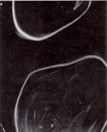
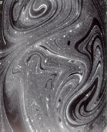
Figure 1: .

Pictures of tracer distributions from experiments. Left: laminar case. Right: fractal case. From Sommerer [2].

Figure 3: The trajectory of an advected particle for different values of $\theta$ in the same $h$-field. From upper right to lower right $\theta=\{0^{\circ},18^{\circ},72^{\circ},90^{\circ}\}$. The particle moved for $90$ time units. From the numerical solution of the 2D Kuramoto-Sivashinsky equation, the field $h$ is known only at discrete points in space. To find the values of the velocity field at all points in space, making the $h$-field a continuous function we used bicubic spline interpolation [10]. This is a standard method for interpolating a function which is only known at discrete points. The interpolated function returned has continuous derivatives.

Figure 4: The two Lyapunov exponents of the particle motion for different values of $\theta$ are shown as the two lower curves. The upper curve show the Lyapunov dimension as calculated from the Kaplan-Yorke conjecture when one Lyapunov exponent is positive. The data points are the measured dimensions of the attractors from the simulations

Figure 5: The measured information dimension at different times for each of the four used values of $\theta$. The horizontal lines are the corresponding calculated Lyapunov dimensions $D_{L}$. It is seen how the values of the measured dimensions apparently converge to the calculated Lyapunov dimensions for the three highest values of $\theta$. For the lowest value of $\theta$, near the threshold of chaos, the dimension of the particle distribution apparently does not converge in time. The fits could seldomly be done over more than one decade, due to cross-over effects at each end of the interval. The limitations are mainly due to computional problems of handling more than the 190.000 particles used.

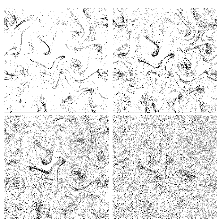
Figure 6: A realization of the particle patterns at time $t=60$. Values of $\theta$ from upper left to lower right: $76.5^{\circ},81.0^{\circ},85.5^{\circ},87.75^{\circ}$. The measured dimensions are from upper left to lower right $1.309\pm 0.005,1.601\pm 0.008,1.873\pm 0.006,1.957\pm 0.005$.

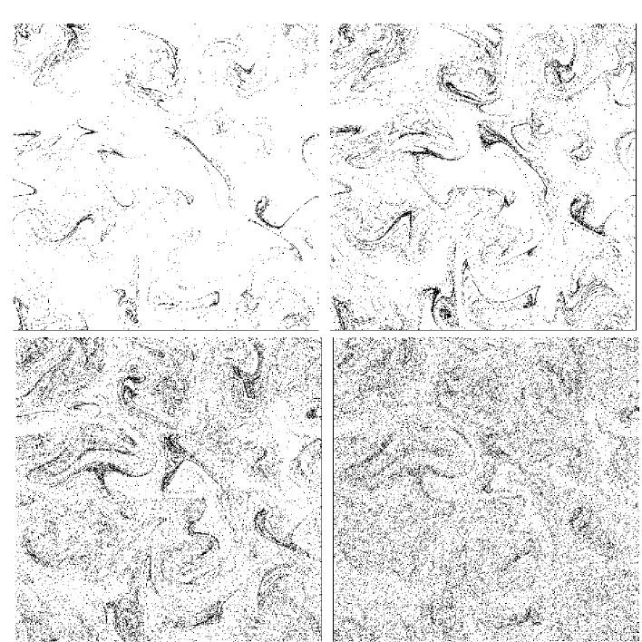
Figure 7: A realization of the particle patterns at time $t=180$. Values of $\theta$ from upper left to lower right: $76.5^{\circ},81.0^{\circ},85.5^{\circ},87.75^{\circ}$. The measured dimensions are from upper left to lower right $0.979\pm 0.007,1.49\pm 0.008,1.821\pm 0.004,1.942\pm 0.006$.

References

- [1] J. C. Sommerer and E. Ott. Particles floating on a moving fluid: A dynamically comprehensible physical fractal. Science, 259:335–339, 1993.
- [2] J. C. Sommerer. Fractal tracer distributions in complicated surface flows: an application of random maps to fluid dynamics. Physica D, 76:85–98, 1994.
- [3] L. Yu, E. Ott, and Q. Chen. Phys. Rev. Lett., 65:2935, 1990.
- [4] L. Yu, E. Ott, and Q. Chen. Physica D., 53:102, 1991.
- [5] Y. Kuramoto. Chemical Oscillations, Waves, and Turbulence. Springer Verlag, 1984.
- [6] G. I. Sivashinsky. Nonlinear analysis of hydrodynamic instability in laminar flames–i. derivation of basic equations. Acta Astronautica, 4:1177–1206, 1977.
- [7] T. Bohr and A. Pikovsky. Anomalous diffusion in the Kuramoto-Sivashinsky equation. Phys. Rev. Lett., 70:2892, 1993.
- [8] E. Ott. Chaos in dynamical systems. Cambridge University Press, 1993.
- [9] G. Benettin, L. Galgani, A. Giorgilli, and J.-M. Strelcyn. Lyapunov Characteristic Exponents for Smooth Dynamical Systems and for Hamiltonian Systems: A Method for Computing All of Them. Part 2: Numerical Application. Meccanica, 15:22, 1980.
- [10] W.H. Press, S.A. Flannery, B.P.and Teukolsky, and W.T. Vetterling. Numerical Recipes in C. Cambridge University Press, second edition, 1992.
- [11] G. Huber, E. Schröder, and P. Alstrøm. Self-diffusion and relative diffusion in defect turbulence. Physica D, 96:1–8, 1996.