An Infinite Step Billiard

Abstract

A class of non-compact billiards is introduced, namely the infinite step billiards, i.e., systems of a point particle moving freely in the domain $\Omega=\bigcup_{n\in{{N}}}[n,n+1]\times[0,p_{n}]$, with elastic reflections on the boundary; here $p_{0}=1,\ p_{n}>0$ and $p_{n}\searrow 0$.

After describing some generic ergodic features of these dynamical systems, we turn to a more detailed study of the example $p_{n}=2^{-n}$. What plays an important role in this case are the so called escape orbits, that is, orbits going to $+\infty$ monotonically in the $X$-velocity. A fairly complete description of them is given. This enables us to prove some results concerning the topology of the dynamics on the billiard.

1 Introduction

Billiards are dynamical systems defined by the uniform motion of a point inside a domain with elastic reflections at the boundary, such that the tangential component of the velocity remains constant and the normal component changes sign. The aim of this paper is to discuss some topological properties for a certain class of non-compact, polygonal billiards, like the one depicted in Fig. 1.

Our main motivations originate from semiclassical quantum mechanics: for example, it would be interesting to compare classical and quantum localization for simple models of non-compact systems. More ambitiously, one might work in the direction of the semiclassical asymptotics for the spectrum of the Hamiltonian operator: the Gutzwiller trace formula and other semiclassical expansions [Gu] relate this to the distribution of periodic orbits in the classical system. In the case of systems with cusps, similar to the ones with which we are concerned here, these types of approximations become more complicated, and one hopes to get a better understanding from the knowledge of the trajectories falling into the cusp (escape orbits; see [Le] and references therein).

Finally, we believe that the investigation of the dynamical properties of such kinds of models inherits an intrinsic interest by itself.

In the case of a bounded polygonal billiard with a finite number of sites, the billiard flow can be studied with the help of some well developed and non-trivial techniques. We refer to [G2, G3] for the basic definitions and results, reducing here to a brief and incomplete review of some of them. Usually one assumes that the magnitude of the particle’s velocity equals one, and that the orbit which hits a vertex stops there (for our model, we will slightly modify this last assumption). However, the set of initial conditions whose orbits are defined for all values of $t$, always represents a set of full measure in the phase space.

Among the class of polygonal billiards, a billiard table $\Omega$ is a rational billiard if the angles between the sides of $\Omega$ are all of the form $\pi n_{i}/m_{i}$, where $n_{i}$ and $m_{i}$ are arbitrary integers. In this case, any orbit will have only a finite number of different angles of reflections. Referring to [G3] for a nice review of the subject, we just note here that this rational condition implies a decomposition of the phase space in a family of flow-invariant surfaces $R_{\theta},\ 0\leq\theta\leq\pi/m,\ m:={\em l.c.m.\,\{m_{i}\}}$, planar representations of which are obtained by the usual unfolding procedure for the orbits (see, e.g., [FK, ZK]). Excluding the particular cases $\theta=0,\pi/m$, it is well known that the billiard flow restricted to any of the $R_{\theta}$ is essentially equivalent to a geodesic flow $\phi_{\theta}^{t}$ on a closed oriented surface $S$, endowed with a flat Riemannian metric with conical singularities. The topological type of the surface $S$ (tiled by $2m$ copies of $\Omega$), i.e., its genus $g$, is determined by the geometry of the rational polygon. For example, if $\Omega$ is a simple polygon, then

$$g(S)=1+\frac{m}{2}\sum_{i=1,n}\frac{n_{i}-1}{m_{i}}.$$ (1)

With the use of this equivalence, a number of theorems regarding the existence and the number of ergodic invariant measures for the flow have been proven ([ZK] and references).

More refined results concerning the billiard flows can then be obtained by exploring the analogies of these flows with the interval exchange transformations (using the induced map on the boundary) on one hand, and with holomorphic quadratic differentials on compact Riemann surfaces, on the other.

The deep connections between these three different subjects have been proven very useful in the understanding of polygonal billiard flows. In particular, we can summarize some of the most important statements in the next proposition (see [G3] and references therein). [Briefly, let us recall that an almost integrable billiard is a billiard whose table is a finite connected union of pieces belonging to a tiling of the plane by reflection, e.g, a rectangular tiling, or a tiling by equilateral triangles, etc.]

Proposition 1

The following statements hold true:

• [KMS, Ar] The Lebesgue measure in a (finite) rational polygon is the unique ergodic measure for the billiard flow, for (Lebesgue-)almost all directions.

• [ZK] For all but countably many directions, a rational polygonal billiard is minimal (i.e., all infinite semi-orbits are dense).

• [G1, G2, B] For almost integrable billiards, “minimal directions” and “ergodic directions” coincide.

• [GK] Let ${\cal{R}}_{n}$ be the space of $n$-gons such that their sides are either horizontal or vertical, parametrized by the length of the sides. Then for any direction $\theta$, $0<\theta<\pi/2$, there is a dense $G_{\delta}$ in ${\cal{R}}_{n}$, such that for each polygon of this set the corresponding flow $\phi_{\theta}^{t}$ is weakly mixing.

• [Ka] For any rational polygon and any direction $\theta$, the billiard flow $\phi_{\theta}^{t}$ is not mixing.

Moreover, by approximating generic polygons by rational ones, other important results can be proven (we still refer to [G3] for a more exhaustive review):

Proposition 2

The following statements hold true:

• [ZK] The set of transitive polygons is a dense $G_{\delta}$.

• [KMS] For every $n$, there is a dense $G_{\delta}$ of ergodic polygons with $n$ vertices.

• [G3] For any given polygon, the metric entropy with respect to any flow-invariant measure is zero.

• [GKT] Given an arbitrary polygon and an orbit, either the orbit is periodic or its closure contains at least one vertex.

In this paper we are interested in a class of rational billiards, the infinite step billiards, defined as follows: let $\{p_{n}\}_{n\in{{N}}}$ be a monotonically vanishing sequence of positive numbers, with $p_{0}=1$. We denote $\Omega:=\bigcup_{n\in{{N}}}[n,n+1]\times[0,p_{n}]$ (Fig. 1) and we call $(X,Y)$ the two coordinates on it.

Following all the above considerations, we see that a point particle can travel within $\Omega$ only in four directions (two if the motion is vertical or horizontal—cases which we disregard). One of these directions lies in the first quadrant. Therefore, for $\theta\in]0,\pi/2[$ and $\alpha=\tan\theta$, the invariant surface is labeled by $R_{\alpha}$ and is built via the unfolding procedure with four copies of $\Omega$. It can be represented on a plane $(X,Y)$ as in Fig.2, with the proper side identifications, and the $3\pi/2$ corners represent the non-removable singularities. With the additional condition $\sum_{n}p_{n}<\infty$, $R_{\alpha}$ can be considered a non-compact, finite-area surface of infinite genus.

We will denote by $\Omega^{(n)}$ the truncated billiard that one obtains by closing the table at $X=n$. The corresponding invariant surface will be obviously denoted by $R_{\alpha}^{(n)}$ (Fig. 3) and (1) shows that it has genus $n$. Only to $R_{\alpha}^{(n)}$ can we apply the many strong statements of Proposition 1 (see also Proposition 3 below). Hence our interest in trying to extend some of those results to the non-compact case. This paper gives a contribution in this direction.

After showing that examples can be given of infinite billiards with the above ergodic properties, we turn to the study of a billiard with exponentially decreasing rational heights ($p_{n}=2^{-n}$) and we give some description of the topological behavior of its orbits. More precisely, we will first describe the existence and the number of the so-called escape orbits, showing that generically (in the initial directions) there is exactly one trajectory “traveling directly to infinity” (Theorem 2). This result makes use, among other more specific computations, of a suitable family of interval maps (rescaled transfer maps), related to the return map to the first vertical wall. With the same tools, we then obtain a characterization of the behavior in the past for these unique escape orbits (Theorem 3). Finally, we analyze some topological properties for the flow associated to the infinite billiard. The main outcome concerning this part is that the dynamics of the whole system is driven by the escape orbit which turns out to be a topologically complex object (Theorem 4).

1.1 General results

Concerning the truncated billiards, we can put together some of the previous results to state the following:

Proposition 3

Fix $n\in{{N}}$ and suppose $p_{k}\in{{Q}},\,\forall k\leq n$. Consider the billiard $\Omega^{(n)}$. If $\alpha\in{{Q}}$, all the trajectories are periodic. If $\alpha\not\in{{Q}}$, the flow is minimal and the Lebesgue measure is the unique invariant ergodic measure.

Proof. As already outlined, this proposition can be derived from quite a number of results in the literature. However, to give an exact reference, [G1], Theorem 3 contains the assertion, since $\Omega^{(n)}$ is an almost integrable billiard table.

It may be interesting to remark that the ideas on which the proofs are based were already known sixty years ago, as [FK] witnesses. The invariant surface $R_{\alpha}^{(n)}$ is divided into a finite number of strips, that are either minimal sets or collections of periodic orbits (the two cases cannot occur simultaneously for an almost integrable billiard). These strips are delimited by generalized diagonals, that is, pieces of trajectory that connect two (possibly coincident) singular vertices of the invariant surface. The above is nowadays called the structure theorem for rational billiards, a sharp formulation of which is found, e.g., in [AG].

Using this, minimality is easily established when, for a given direction, no generalized diagonals and no periodic orbits are found. Q.E.D.

The above proposition will be used repeatedly during the remainder, being more or less the only result we can borrow from our (much wider) knowledge of the compact case. One of the first statements we can derive from it is that we can actually find examples of step billiards which enjoy the ergodic properties one would expect. The price we pay is that we must let the system decide, for a given irrational direction, how fast the $p_{n}$’s should decay.

Theorem 1

Fix $\alpha\not\in{{Q}}$. For every positive vanishing sequence $\{\bar{p}_{n}\}$, there exists a strictly decreasing sequence $\{p_{n}\}\subset{{Q}}$, with $0<p_{n}\leq\bar{p}_{n}$, such that the billiard flow $\phi_{\alpha}^{t}$ on $R_{\alpha}$, constructed as above according to $\{p_{n}\}$, is ergodic (hence almost all orbits are dense).

The proof of this theorem is postponed to the next section, after we have established some further notation.

Another useful result can be derived from Proposition 3:

Proposition 4

Let an infinite step billiard $\Omega$ with rational heights ($p_{n}\in{{Q}},\>\forall n$) be given. If $\alpha\in{{Q}}$, a semi-orbit can be either periodic or unbounded. If $\alpha\not\in{{Q}}$, all semi-orbits are unbounded.

Proof. If $\alpha\in{{Q}}$ and we had a non-periodic bounded trajectory, this would naturally correspond to a trajectory of $R_{\alpha}^{(n)}$, for some $n\in{{N}}$, which has only periodic orbits. On the other hand, if $\alpha\not\in{{Q}}$, the dynamics over each $R_{\alpha}^{(n)}$ is minimal. Hence, every semi-trajectory reaches the abscissa $X=n$. Q.E.D.

1.2 The Return Map

In our realization of the surface $R_{\alpha}$, the first vertical side of $\Omega$ becomes the closed curve $L:=\{0\}\times[-1,1[$ [$(0,-1)$ e $(0,1)$ are identified in Fig. 2] which separates $R_{\alpha}$ in two symmetric parts. We will occasionally identify $L$ with the interval $[-1,1[$.

Except for the trivial case $\alpha=+\infty$ (vertical orbits—already excluded at the beginning), every trajectory crosses $L$ at least once. Without loss of generality, we will always assume to have an initial point $(0,Y_{0})$ on the leftmost wall $L$, uniquely associated to a pair $(Y_{0},\alpha)\in[-1,1[\times]0,+\infty[$. We then use the Lebesgue measure as a natural way to measure orbits.

The billiard flow along a direction $\alpha$, which we denote by $\phi_{\alpha}^{t}$ (or $\phi^{t}$ when there is no means of confusion), induces a.e. on $L$ a Poincaré map $P_{\alpha}$ that preserves the Lebesgue measure. We call it the (first) return map. This discontinuous map is easily seen to be an infinite partition interval exchange transformation (i.e.t.). On $L$ we establish the convention that the map is continuous from above: i.e., an orbit going to the singular vertex $(n,p_{n})$ of $R_{\alpha}$ will continue from the point $(-n,p_{n})$, thus behaving like the orbits above it, i.e., bouncing backwards. In the same spirit, a trajectory hitting $(-n,p_{n})$ will continue from $(-n,-p_{n})$, while orbits encountering vertex $(n,-p_{n})$ will just pass through. This corresponds to partitioning $L\simeq[-1,1[$ into right-open subintervals.

The fact that the number of subintervals is infinite is exactly what makes the study of the ergodic properties of this system a non-trivial task.

It is now natural to relate $P_{\alpha}$ to the family of return maps $P_{\alpha}^{(n)}$ corresponding to the truncated billiards $\Omega^{(n)}$. These are finite partition i.e.t.’s defined on all of $L$ (with abuse of notation, $L$ also denotes the obvious closed curve on $R_{\alpha}^{(n)}$, Fig. 3).

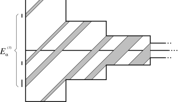
Figure 4: Construction of $E_{\alpha}^{(n)}$ as the backward evolution of the “aperture” $G_{n}$. The beam of orbits may split at singular vertices.

Let $E_{\alpha}^{(n)}\subset L$ be the set of points whose forward orbit starts along the direction $\alpha$ and reaches the $n$-th aperture $G_{n}:=\{n\}\times[-p_{n},p_{n}[$ without colliding with any vertical walls. $E_{\alpha}^{(n)}$ is union of at most $n$ right-open intervals, since the backward evolution of $G_{n}$ can only split once for each of the $n-1$ singular vertices (Fig. 4). We denote this by $n.i.(E_{\alpha}^{(n)})\leq n$, where $n.i.$ stands for “number of intervals”. Moreover, $|E_{\alpha}^{(n)}|=2p_{n}$ and $E_{\alpha}^{(n+1)}\subset E_{\alpha}^{(n)}$. From this we infer that the family $\{E_{\alpha}^{(n)}\}_{n>0}$ can be rearranged into sequences of nested right-open intervals, whose lengths vanish as $n\to\infty$. Clearly, the sequence of i.e.t.’s $P_{\alpha}^{(n)}\to P_{\alpha}$ a.e. in $L$ as $n\to\infty$.

The subset of $L$ on which $P_{\alpha}$ is not defined will be denoted by $E_{\alpha}:=\bigcap_{n>0}E_{\alpha}^{(n)}$ and clearly $|E_{\alpha}|=0$ . Each point of this set is the limit of an infinite sequence of nested vanishing right-open intervals (the constituents of the sets $E_{\alpha}^{(n)}$). Elementary topology arguments allow us to assert an almost converse statement: each infinite sequence yields a point of $E_{\alpha}$, unless the “pathological” property holds that the intervals eventually share their right extremes.

The orbits starting from such points will never collide with any vertical side of $R_{\alpha}$ (or $\Omega$) and thus, as $t\to+\infty$, will go to infinity, maintaining a positive constant $X$-velocity. We call them escape orbits.

We now give the proof of Theorem 1.

1.3 Proof of Theorem 1

We will construct $R_{\alpha}$ in such a way that almost every point in $L$ has a typical trajectory, in the sense that the time average of a function in a dense subspace of $L^{1}(R_{\alpha})$ equals its spatial average. Since $L$ is a Poincaré section, the same property will hold for a.e. point in $R_{\alpha}$. For the sake of notation, we will drop the subscript $\alpha$ in the sequel.

Take a positive sequence $\varepsilon_{n}\searrow 0$. We are going to build our billiard by induction: suppose we have fixed $p_{i}$ for $1\leq i\leq n$, and we have to determine a suitable $p_{n+1}$. Consider $R^{(n)}$, generated by the $p_{i}$’s found so far. The flow $\phi_{(n)}^{t}$ on it is ergodic by Proposition 3. For $f\in L^{1}(R^{(n)})$ and $z\in L$ define

$$\left(\Xi_{(n)}^{T}f\right)(z):=\frac{1}{T}\int_{0}^{T}f\circ\phi_{(n)}^{t}(z)\,dt-\frac{1}{|R^{(n)}|}\int_{R^{(n)}}f\,dXdY.$$ (2)

Let $\{f_{j}^{(n)}\}_{j\in{{N}}}$ be a separable basis of $L^{1}(R^{(n)})$. For the rest of the proof $R^{(n)}$ will be liberally regarded as an (open) submanifold of $R^{(m)},m>n$. As a consequence, a function defined on the former set will be implicitly extended to the latter by setting it null on the difference set. With this in mind, let

$$A_{T}^{(n)}:=\left\{z\in L\,|\,\forall\,1\leq i,j\leq n,\left|\,\Xi_{(n)}^{T}f_{i}^{(j)}(z)\,\right|\leq\varepsilon_{n}\right\}.$$ (3)

By ergodicity, since only a finite number of functions are involved in the above set, we have $|A_{T}^{(n)}|\to|L|=2$ as $T\to\infty$. Take $T_{n}$ such that $|A_{T_{n}}^{(n)}|\geq 2-\varepsilon_{n}/2$. We are now in position to determine $p_{n+1}$. Choose some

$$p_{n+1}\in{{Q}};\ 0<p_{n+1}\leq\min\left\{\bar{p}_{n+1},\frac{\varepsilon_{n}}{2T_{n}}\right\},$$ (4)

and imagine to open a hole of width $2p_{n+1}$ in the middle of $\{n+1\}\times[-p_{n},p_{n}[$ (same as $\{-n-1\}\times[-p_{n},p_{n}[$ since they are identified at the moment). The motion on $R^{(n)}$ is not affected very much by this change, during the time $T_{n}$. If we denote by $\phi^{t}$ the flow on the infinite billiard table (when we are done constructing it), we can already assert that, taken a point $z\in L$, $\phi_{(n)}^{t}(z)=\phi^{t}(z)\,\forall t\in[0,T_{n}]$ unless the particle departing form $z$ hits the hole in a time less than $T_{n}$. We can estimate the measure of these “unlucky” initial points: they constitute the set

$$B_{n}:=L\cap\left(\bigcup_{t\in[-T_{n},0]}\phi_{(n)}^{t}(\{n+1\}\times[-p_{n+1},p_{n+1}[\,)\right).$$ (5)

The backward beam (up to time $-T_{n}$) originating from the hole cannot hit $L$ more than $T_{n}/2$ times, since between each two successive crossings of $L$, the beam has to cover a distance which is at least 2 (see Fig. 3), but the velocity of the particles was conventionally fixed to 1. Every intersection of the beam with $L$ is a set of measure $2p_{n+1}$, so, from (4), $|B_{n}|\leq\varepsilon_{n}/2$.

Set $C_{n}:=A_{T_{n}}^{(n)}\setminus B_{n}$, thus $|C_{n}|\geq 2-\varepsilon_{n}$. So $C_{n}$ is the set of points which keep enjoying the properties as in (3), even after the cut has been done in $R_{(n)}$. Suppose one repeats the above recursive chain of definitions for all $n$ in order to define the infinite manifold $R$. Let $C:=\bigcap_{n\in{{N}}}\bigcup_{m\geq n}C_{m}$. Then $|C|=\lim_{n\to\infty}\cup_{m\geq n}C_{m}=2=|L|$. $C$ may be called the event $\{\{C_{n}\}$ infinitely often$\}$; it is the “good” set since, fixed $z\in C$, there exist a subsequence $\{n_{k}\}$ such that $z\in\bigcap_{k}C_{n_{k}}$. This means that, taken two integers $i,j$, $\forall n_{k}\geq\max\{i,j\}$,

$$\left|\frac{1}{T_{n_{k}}}\int_{0}^{T_{n_{k}}}f_{i}^{(j)}\circ\phi^{t}(z)\,dt-\frac{1}{|R^{(n_{k})}|}\int_{R}f_{i}^{(j)}\,dXdY\right|\leq\varepsilon_{n_{k}}.$$ (6)

Comparing this with (2) we notice two differences. First, the flow that appears here is $\phi^{t}$ because of the remark after (4). Second, the manifold integral is taken over all of $R$: this is so because of the initial convention to extend with zero all functions defined on submanifolds of $R$.

Define $\Xi^{T}$ in analogy with (2). Since $|R^{(n)}|\nearrow|R|$, (6) shows that $(\Xi^{T_{n_{k}}}f_{i}^{(j)})(z)\to 0$, as $k\to\infty$, with $T_{n}$ in general going to $\infty$ (this is not indeed guaranteed by the definition of $T_{n}$, but one can easily arrange to make this happen). We would not be done yet, if it were not for Birkhoff’s Theorem, which states that, for the function $f_{i}^{(j)}\in L^{1}(R)$, the time average is well-defined a.e. (in $R$, hence in $L$). Summarizing, for every $f\in{\rm span}\{f_{i}^{(j)}\}_{i,j\in{{N}}}$, there exists a set $C_{f}\subseteq L,\,|C_{f}|=2$ such that

$$\lim_{T\to+\infty}(\Xi^{T}f)(z)=0.$$ (7)

This proves the claim we made in the beginning. Since $\Xi^{T}$ is a continuous operator in $L^{1}$ and ${\rm span}\{f_{i}^{(j)}\}$ is dense in it, we obtain the ergodicity part in the statement of Theorem 1. As concerns the density result, this immediately follows from standard arguments as in [W], Theorem 5.15 (which can be checked to hold under our hypotheses, as well). Q.E.D.

Remark. The fact that the above result provides ergodic billiards with rational heights only is merely technical. We decided to use Proposition 3, which only deals with almost integrable billiards. For a generic finite step billiard one can as well say that for almost all directions the flow is ergodic, by [KMS], and a slight generalization of Theorem 1 can be proven in a hardly different way.

2 The Exponential Step Billiard

Our main example of step billiard, to which we will restrict our attention for the rest of this paper, is the exponential step billiard, i.e., the case $p_{n}=2^{-n}$, shown in Figs. 1, 2, 3.

We are, of course, interested in getting information about the unbounded orbits of our non-compact dynamical system over $\Omega$, since bounded orbits correspond to a billiard $\Omega^{(n)}$, for some $n\in{{N}}$. Indeed, Proposition 4 applies here allowing one to conclude that (for almost all $\alpha$’s) all but a countable set of initial conditions on $L$ give rise to unbounded orbits, which come back to $L$ infinitely often.

We will first focus on the escape orbits, as introduced in Section 1.2. Strictly speaking, we consider only the asymptotic behavior of the forward semi-orbit. But a glance at Fig. 2 at once shows that the backward semi-orbit having initial conditions $(Y_{0},\alpha)$ is uniquely associated, by symmetry around the origin, to the forward semi-orbit of $(-Y_{0},\alpha)$.

Remark. The above assertion needs to be better stated: although the manifold $R_{\alpha}$ is symmetric around the origin, the flow defined on it is not exactly invariant for time-reversal, as Fig. 2 seems to suggest. This is due to our convention in Section 1.2 about the continuity from above for the flow. The time-reversed motion on $R_{\alpha}$ is isomorphic to the motion on a manifold like $R_{\alpha}$ with the opposite convention (continuity from below). Nevertheless, little changes since only singular orbits (a null-measure set) are going to be affected by this slight asymmetry.

We will characterize the existence and the number of the escape orbits and we will show that, generically, only one of the two branches of an orbit can escape (see Section 2.2). Moreover, we borrow some notation from [L] and call oscillating all unbounded non-escape (semi-)orbits.

For the moment, let us introduce the following construction: suppose that a trajectory $\gamma$ on $R_{\alpha}$ reaches directly, that is monotonically in the $X$-coordinate, the opening $G_{n}=\{n\}\times[-2^{-n},2^{-n}[$. Let us denote with $Y_{n}\in[-2^{-n},2^{-n}[$ the ordinate of the point at which $\gamma$ crosses $G_{n}$. Within the box $]n,n+1[\times[-2^{-n},2^{-n}[$, the motion is a simple translation. Hence

$$Y_{n+1}=Y_{n}+\alpha\ ({\rm mod}\ {2^{-n+1}}),$$ (8)

with$\ ({\rm mod}\ {r})$ meaning the unique point in $[-r/2,r/2[$ representing the class of equivalence in ${{R}}/r{{Z}}$, rather than the class of equivalence itself. The trajectory $\gamma$ will cross $G_{n+1}$ if, and only if,

$$Y_{n+1}\in[-2^{-(n+1)},2^{-(n+1)}[.$$ (9)

Setting $y_{n}:=2^{n-1}Y_{n}$, relation (8) becomes

$$y_{n+1}=2y_{n}+2^{n}\alpha\ ({\rm mod}\ 2),$$ (10)

and the trajectory will cross $G_{n+1}$ if, and only if,

$$y_{n+1}\in\left[-\frac{1}{2},\frac{1}{2}\right[.$$ (11)

The recursion relation (10) can be easily proven by induction to yield

$$y_{n+1}=2^{n+1}y_{0}+(n+1)2^{n}\alpha\ ({\rm mod}\ 2),$$ (12)

where the numbers $y_{k}\in[-1/2,1/2[$ now represent the (rescaled) intersections of the trajectory with the vertical openings $G_{k}$.

The transformation $T_{n,\alpha}:[-1/2,1/2[\,\longrightarrow[-1,1[$,

$$T_{n,\alpha}(y):=2y+2^{n}\alpha\ ({\rm mod}\ 2)$$ (13)

will be called the rescaled transfer map.

2.1 Escape Orbits

In this section we shall exploit the escape orbits for the exponential step billiard $\Omega$ defined above. Actually, we will give a rather complete description of what happens to the set $E_{\alpha}$, as defined in Section 1.2, for $\alpha>0$. We already know that $|E_{\alpha}|=0$. Among more detailed results, we will show that $E_{\alpha}$ can only contain one or two points, the former case holding for almost all directions $\alpha$.

We start with some easy statements, using rescaled coordinates, unless otherwise specified.

Lemma 1

If $\alpha=2k$, $k\in{{Z}}$, only one escape orbit exists and its initial condition is $y_{0}=0$.

Proof. $T_{n,2k}=T_{n,0}\ \forall n\in{{N}}$. The sequence $\{y_{n}\}$ is in this case given by $y_{n}=2^{n}y_{0}\ ({\rm mod}\ 2)$. If $y_{0}=0$, all $y_{n}$ are null and the corresponding trajectory escapes, according to (11). If $y_{0}\neq 0$, there exists a $k$ such that $|y_{k}|>1/2$. Q.E.D.

In Fig. 2, designate by $V_{n}$ the point $(n,-2^{-n}),\ n\geq 0$. For $n\geq 1$, this means that, on the planar representation of $R_{\alpha}$, $V_{n}$ is the one copy of the $n$-th singular vertex of $\Omega$, such that its future semi-orbit is going “to the right”.

Corollary 1

If $\alpha=k\,2^{-j}$, with $k$ odd, $j$ non-negative integer, only one escape orbit occurs. This orbit intercepts $V_{j}$.

Proof. The portion of the manifold $R_{\alpha}$ at the right of the $(j+1)$-th aperture looks like $R_{\alpha}$ itself, modulo a scale factor equal to $2^{-(j+1)}$. Furthermore in that region, and subject to the above rescaling, the transfer map is equivalent to the one we have seen in the previous lemma. In fact, for $n\geq j+1$, $T_{n,\alpha}=T_{n,0}$. So, to the part of the escape orbit after $G_{j+1}$, we can apply that lemma and conclude that the escape trajectory is unique and $y_{j+1}=0$ holds. Now, we know that $\alpha$ is indeed equal to $(2k^{\prime}+1)2^{-j}$. Inverting (10) with $y_{j+1}=0$, we get $y_{j}=-k^{\prime}-1/2-p$, for some integer $p$. By (11) $y_{j}\in[-1/2,1/2[$. Hence $y_{j}=-1/2$, which proves the second part of the lemma. Q.E.D.

In Lemma 1 we have encountered the case in which $\{T_{n,\alpha}\}$ is a sequence of identical maps. Considering the more general case of a periodic sequence of maps will yield a useful tool to detect the presence of more than one escape orbit.

Observe that, when $\alpha=2k/(2^{m}-1)$ with $k,m$ positive integers, one gets $2^{m}\alpha=\alpha\ ({\rm mod}\ 2)$. In this case we have a periodic sequence of transfer maps of period $m$, that is, $T_{pm,\alpha}=T_{0,\alpha}$ for all integer $p>0$. For such directions, then, one method for detecting escape orbits may be the following: Let us set $M_{m,\alpha}:=T_{m-1,\alpha}\circ\>\cdots\>\circ T_{0,\alpha}$. As in (12) it turns out that $M_{m,\alpha}(y)=2^{m}y+m2^{m-1}\alpha\ ({\rm mod}\ 2)$. Let us now find the fixed points of this map. Consider a trajectory having one of these points as initial datum. If it crosses all openings between $G_{1}$ and $G_{m}$, then the sequence of crossing points $y_{0},\ldots,y_{m-1}$ will be indefinitely repeated and the trajectory will escape.

Let us apply this technique to the case $k=1$ and $m=2$, that is $\alpha=2/3$. Hence the fixed points of the map $M_{2,2/3}$ are the points $y\in[-1,1[$ such that $y=4y+8/3+2p,\>p\in{{Z}}$. They are

$$y^{(0)}=-\frac{8}{9};\ \ y^{(1)}=-\frac{2}{9};\ \ y^{(2)}=\frac{4}{9}.$$ (14)

Since $|y^{(0)}|=|M_{2,2/3}\,y^{(0)}|>1/2$, that solution has to be discarded. Instead, $y^{(1)}=:y^{(1)}_{0}$ is accepted since

$$y^{(1)}_{1} = 2y^{(1)}_{0}+\frac{2}{3}\ ({\rm mod}\ 2)=\frac{2}{9}\in\left[-\frac{1}{2},\frac{1}{2}\right[$$

$$y^{(1)}_{2} = y^{(1)}_{0}\in\left[-\frac{1}{2},\frac{1}{2}\right[.$$ (15)

It turns out that the same holds for $y^{(2)}$.

Thus, for $\alpha=2/3$ there are at least two escape orbits whose initial conditions in the non-rescaled coordinates are $Y_{0}=-4/9$ and $Y_{0}=8/9$. As orbits of $R_{\alpha}$ they are distinct, but is this still true if we consider the corresponding orbits in the billiard $\Omega$?

Lemma 2

For $\alpha=2/3$, the two escape orbits with initial conditions $Y_{0}=-4/9$ and $Y_{0}=8/9$ have distinct projections on $\Omega$.

Proof. Suppose that the two escape orbits coincide in $\Omega$. Then the backward part of the orbit, that starts at $Y=-4/9$, must get to $Y=8/9$, after several oscillations. According to the fact that a backward semi-orbit having initial condition $(Y_{0},\alpha)$ is associated to the forward semi-orbit $(-Y_{0},\alpha)$ (see remark at the beginning of Section 2), the geometry of $R_{\alpha}$ implies that

$$\frac{8}{9}=-\frac{4}{9}+\sum_{i=1}^{j}\left(\frac{2}{3}-\frac{m_{i}}{2^{q_{i}}}\right),$$ (16)

where $m_{i},q_{i}$ are non-negative integers and $j$ is the number of rectangular boxes visited by the backward semi-orbit before reaching the point with coordinate $Y=8/9$. [We remind that in each box the variation of the $Y$-coordinate is $\alpha\ ({\rm mod}\ {2^{-q_{i}}})$.] Rearranging this formula we obtain

$$\frac{4}{9}=\frac{2}{3}j-\frac{m}{2^{q}},$$ (17)

for some non-negative integers $m$ and $q$. For any choice of $m,q$ and $j$, the two sides are distinct. This contradicts our initial assumption that the two orbits coincide. Q.E.D.

We will see later in Corollary 2 that, along any direction $\alpha$, there are no more than two escape orbits in $R_{\alpha}$. We can summarize everything about the case $\alpha=2/3$ in the following assertion.

Proposition 5

Along the direction $\alpha=2/3$ there are two distinct escape orbits.

We now turn to the study of the generic case. Recalling the reasoning outlined in Section 1.2 about the splitting of the backward beams of orbits (see also Fig. 4), it comes natural to think that at this point we need to analyze the forward trajectories starting from the singular vertices $V_{p}=(p,-2^{-p})$. We name them $\gamma_{p}$.

First of all, we consider those $\alpha$’s for which $\gamma_{0}$ reaches directly $G_{n}$, i.e., before hitting any vertical wall: we look at Fig. 5, which displays the “unfolding” of $R_{\alpha}$, (where an orbit over $R_{\alpha}$ is turned into a straight line). A direct evaluation with a ruler, furnishes the answer, that runs as follows:

$$n=1)\ \frac{1}{2}\leq\alpha\ ({\rm mod}\ 2)<\frac{3}{2}$$ (24)

$$n\geq 2)\ \left\{\begin{array}[]{l}\displaystyle{\frac{1}{2}\leq\alpha\ ({\rm mod}\ 2)<\frac{1}{2}+\frac{1}{n2^{n}};}\\ \\ \displaystyle{1-\frac{1}{n2^{n}}\leq\alpha\ ({\rm mod}\ 2)<1+\frac{1}{n2^{n}};}\\ \\ \displaystyle{\frac{3}{2}-\frac{1}{n2^{n}}\leq\alpha\ ({\rm mod}\ 2)<\frac{3}{2}.}\end{array}\right.$$

Due to the self-similarity of our infinite billiard, we can write down the analogous inequalities for every other vertex $V_{p},\,p\geq 1$ by rescaling (24) and (24). Thus $\gamma_{p}$ crosses $G_{m},\ m>p$ if, and only if,

$$m=p+1)\ \!\frac{1}{2^{p+1}}\leq\alpha\ ({\rm mod}\ {2^{-p+1}})<\frac{3}{2^{p+1}}$$ (31)

$$m\geq p+2)\ \!\left\{\begin{array}[]{l}\displaystyle{\frac{1}{2^{p+1}}\leq\alpha\ ({\rm mod}\ {2^{-p+1}})<\frac{1}{2^{p+1}}\!+\!\frac{1}{(m\!-\!p)2^{m}};}\\ \\ \displaystyle{\frac{1}{2^{p}}\!-\!\frac{1}{(m\!-\!p)2^{m}}\leq\alpha\ ({\rm mod}\ {2^{-p+1}})<\frac{1}{2^{p}}\!+\!\frac{1}{(m\!-\!p)2^{m}};}\\ \\ \displaystyle{\frac{3}{2^{p+1}}\!-\!\frac{1}{(m\!-\!p)2^{m}}\leq\alpha\ ({\rm mod}\ {2^{-p+1}})<\frac{3}{2^{p+1}}.}\end{array}\right.$$

Working out these relations is essentially all we need to reach the goal we have set for ourselves at the beginning of this section. From now on, when we say that an orbit $\gamma_{p}$ reaches or crosses an aperture $G_{m}$, we will always mean directly.

Lemma 3

If $\gamma_{p}$ is an escape orbit then it is the only escape orbit.

Proof. It follows from (31)-(31) that $\gamma_{p}$ is an escape orbit if, and only if, $\alpha\in\{2^{-p},2^{-p-1}\}\ ({\rm mod}\ {2^{-p+1}})$. But for such $\alpha$’s, Corollary 1 states that there is only one escape orbit. Q.E.D.

Lemma 4

Let $m,p$ be two non-negative integers with $m\geq p+2$. If $\gamma_{p}$ crosses $G_{m}$, then either $\gamma_{p+1}$ does not reach $G_{p+2}$ or it crosses $G_{m}$, as well.

Proof. It suffices to prove the statement for $p=0$ and the reader can easily get convinced that the actual result follows by a rescaling. Set

$$I_{m}^{(1)} := \bigcup_{j\in{{N}}}\left[\frac{1}{2}+2j,\frac{1}{2}+\frac{1}{m2^{m}}+2j\right[,$$

$$I_{m}^{(2)} := \bigcup_{j\in{{N}}}\left[1-\frac{1}{m2^{m}}+2j,1+\frac{1}{m2^{m}}+2j\right[,$$ (32)

$$I_{m}^{(3)} := \bigcup_{j\in{{N}}}\left[\frac{3}{2}-\frac{1}{m2^{m}}+2j,\frac{3}{2}+2j\right[.$$

From (24), $\gamma_{0}$ crosses $G_{m}$ if, and only if, $\alpha\in I_{m}:=I_{m}^{(1)}\cup I_{m}^{(2)}\cup I_{m}^{(3)}$. If $\alpha\in I_{m}^{(2)}$ then $\gamma_{1}$ does not cross $G_{2}$. In fact, (31) states that $\gamma_{1}$ crosses $G_{2}$ if, and only if, $\alpha\in B:=\bigcup_{k\in{{N}}}[1/4+k,3/4+k[$. So we have to prove that the sets $I_{m}^{(2)}$ and $B$ have empty intersection. This is the case, because $I_{m}^{(2)}$ is made up of intervals of center $2j+1$ and radius $1/(m2^{m})$, and $B$ is made up of intervals of center $1/2+k$ and radius $1/4$, so that

$${\rm dist}(I_{m}^{(2)},B)\geq\frac{1}{2}-\left(\frac{1}{m2^{m}}+\frac{1}{4}\right)>0\ \ \ {\rm for}\ m\geq 2.$$ (33)

It remains to analyze the case $\alpha\in C:=I_{m}^{(1)}\cup I_{m}^{(3)}$. Relations (31) tell us that $\gamma_{1}$ crosses $G_{m}$ if, and only if,

$$\alpha\in D:=\bigcup_{k\in{{N}}} \Biggl{(} \left[\frac{1}{4}+k,\frac{1}{4}+\frac{1}{(m-1)2^{m}}+k\right[\cup$$

$$\cup \left[\frac{1}{2}-\frac{1}{(m-1)2^{m}}+k,\frac{1}{2}+\frac{1}{(m-1)2^{m}}+k\right[\cup$$

$$\cup \left[\frac{3}{4}-\frac{1}{m2^{m}}+k,\frac{3}{4}+k\right[\ \ \Biggr{)}.$$

We have to prove that $C\subseteq D$. We can visualize the sets $C$ and $D$ as periodic structures on the line whose fundamental patterns have, respectively, lengths 2 and 1 (with common endpoints). Therefore, defining $\hat{C}:=C\cap[0,2]=[1/2,1/2+1/(m2^{m})[\,\cup\,[3/2-1/(m2^{m}),3/2[$ and $\hat{D}:=D\cap[0,2]$, all we have to do is to show that $\hat{C}\subseteq\hat{D}$. Deducing the shape of $\hat{D}$ from (2.1), the result follows from the trivial relations:

$$\left[\frac{1}{2},\frac{1}{2}+\frac{1}{m2^{m}}\right[ \subset \left[\frac{1}{2}-\frac{1}{(m-1)2^{m}},\frac{1}{2}+\frac{1}{(m-1)2^{m}}\right[,$$ (35)

$$\left[\frac{3}{2}-\frac{1}{m2^{m}},\frac{3}{2}\right[ \subset \left[\frac{3}{2}-\frac{1}{(m-1)2^{m}},\frac{3}{2}+\frac{1}{(m-1)2^{m}}\right[.$$ (36)

Q.E.D.

Lemma 5

Again $m\geq p+2$. If $\gamma_{p}$ crosses $G_{m}$, then for all $p+2\leq n\leq m$, $\gamma_{n}$ does not reach $G_{n+1}$.

Proof. As before, we give the proof only for the case $p=0$. The orbit $\gamma_{0}$ crosses $G_{m}$ if, and only if, $\alpha\in I_{m}$ defined in the proof of the previous lemma, whereas $\gamma_{n}$ crosses $G_{n+1}$ if, and only if,

$$\alpha\in J_{n}:=\bigcup_{k\in{{N}}}\left[\frac{1}{2^{n+1}}+\frac{k}{2^{n-1}},\frac{3}{2^{n+1}}+\frac{k}{2^{n-1}}\right[.$$ (37)

If $I_{m}$ and $J_{n}$ have empty intersection, for all $2\leq n\leq m$, then the lemma is proven. Proceeding as in the first part of Lemma 4, we see that $I_{m}$ is strictly contained in a union of intervals of center $q/2$ and radius $1/(m2^{m})$, while the intervals constituting $J_{n}$ have center $2^{-n}+k2^{-n+1}$ and radius $2^{-n-1}$. Thus, for $3\leq n\leq m$,

$${\rm dist}(I_{m},J_{n})\geq\frac{1}{2^{n}}-\left(\frac{1}{m2^{m}}+\frac{1}{2^{n+1}}\right)>0.$$ (38)

If $n=2$, (38) becomes an equality, but the fact that our intervals are right-open ensures nevertheless that $I_{m}\cap J_{2}=\emptyset$. Q.E.D.

One way to memorize the previous technical lemmas may be as follows. The fact that $\gamma_{p}$ crosses $G_{m}$ influences all $\gamma_{n}$’s, for $n$ between $p+1$ and $m$: if $\gamma_{p+1}$ wants to “take off” (that is, reach some apertures), then it is forced to follow, and possibly pass, $\gamma_{p}$; while the $\gamma_{n}$’s with $n\geq p+2$ cannot even take off.

We now enter the core of the arguments: recall the notation $n.i.$ to designate the number of disjoint intervals that constitute a set.

Lemma 6

Fix $\alpha>0$. Either there exists an integer $q$ such that $n.i.(E_{\alpha}^{(n)})=2$ for all $n\geq q$, or there is a sequence $\{n_{j}\}$ such that $n.i.(E_{\alpha}^{(n_{j})})=1$.

Proof. The set of $\alpha$’s with the property that $n.i.(E_{\alpha}^{(n)})=2$ for $n\geq q$ is not empty. In fact, by direct computation, it is easy to verify that for $\alpha=2/3$ every $\gamma_{n}$ crosses $G_{n+1}$ but not $G_{n+2}$, so that $n.i.(E_{\alpha}^{(n)})=2$ for all $n>0$.

Now, suppose there exists a sequence $\{{m_{j}}\}$ with $n.i.(E_{\alpha}^{(m_{j})})\neq 2$. We can assume $n.i.(E_{\alpha}^{(m_{j})})\geq 3$, otherwise, maybe passing to a subsequence, we would have $n.i.(E_{\alpha}^{(m_{j})})=1$ and we would be done. If we fix an $m_{j}$ there are at least two singular orbits that cross $G_{m_{j}}$. Let $0<p_{j}\leq m_{j}-2$ be the smallest integer such that $\gamma_{p}$ crosses $G_{m_{j}}$. It follows from Lemma 5 that only $\gamma_{p_{j}}$ and $\gamma_{p_{j}+1}$ cross $G_{m_{j}}$. Therefore $n.i.(E_{\alpha}^{(m_{j})})=3$.

At this point we have three cases: $\gamma_{p_{j}}$ and $\gamma_{p_{j}+1}$ are both escape orbits; one of them escapes and the other is reflected; they are both reflected.

In the first case Lemma 3 ensures that $\gamma_{p_{j}}$ and $\gamma_{p_{j}+1}$ coincide and Lemma 5 implies that no $\gamma_{n}$ with $n>p_{j}+1$ can “take off”. Hence $n.i.(E_{\alpha}^{(m)})=2$ for all $n\geq p_{j}+1$, contradicting our assumption. The second case is hardly any different: call $G_{n_{j}}$ the first aperture that $\gamma_{p_{j}}$ cannot reach (in fact Lemma 4 implies that, of the two, $\gamma_{p_{j}+1}$ must be the escaping trajectory). Therefore, using again Lemma 5, $n.i.(E_{\alpha}^{(m)})=2$ for all $n\geq n_{j}$, a contradiction as before. In the last case, call $G_{n_{j}}$ the first aperture which is not reached by $\gamma_{p_{j}+1}$, and thus not even by $\gamma_{p_{j}}$. [Lemma 4 claims that $\gamma_{p_{j}+1}$ goes farther than $\gamma_{p_{j}}$.] Another application of Lemma 5 proves that $n.i.(E_{\alpha}^{(n_{j})})=1$. Proceeding inductively we find a sequence of integers $n_{j}>m_{j}$ with the desired property. Q.E.D.

Corollary 2

For all $\alpha$’s, $\#E_{\alpha}\leq 2$.

Lemma 7

Notation as in the above lemma. In the case $n.i.(E_{\alpha}^{(n)})=2$ for $n\geq q$, suppose $q\geq 1$ is the minimum integer enjoying that property. Then there are only two possibilities:

• $\gamma_{q-1}$ is the only escape orbit and $\alpha=2^{1-q}\ ({\rm mod}\ {2^{2-q}})$.

• $\gamma_{n}$ crosses $G_{n+1}$ but not $G_{n+2}$ for all $n\geq q-1$ so that there are two escape orbits and either $\alpha=2^{2-q}/3\ ({\rm mod}\ {2^{2-q}})$ or $\alpha=2^{3-q}/3\ ({\rm mod}\ {2^{2-q}})$.

Proof. First, let us see that $\gamma_{q-1}$ is the only singular orbit crossing $G_{q}$. In fact $G_{q}$, by hypothesis, is intersected by only one $\gamma_{k}$ ($k\leq q-1$). [Actually, the case may occur that both $\gamma_{p}$ and $\gamma_{k}$ cross that aperture, but only if they coincide. Nothing changes in the argument if we take $k$ to be the largest integer of the two.] If $k\leq q-2$, then by Lemma 5, no singular orbit $\gamma_{n}$, with $n\geq k+2$ can “take off”. Neither can $\gamma_{k+1}$, which would be forced, by Lemma 4, to pass $G_{q}$, against the hypotheses. The net result is that $n.i.(E_{\alpha}^{(n)})=2,\ \forall n\geq k+1$, which contradicts the minimality of $q$.

Now suppose that $\gamma_{q-1}$ reaches $G_{q+1}$. We want to prove that it is also an escape orbit and we are in case (a). In fact, if it stops somewhere after $G_{q+1}$ (say right before $G_{k},\ k>q+1$), then $\gamma_{q}$ either passes it (and $n.i.(E_{\alpha}^{(q+1)})=3$) or $\gamma_{q}$ does not “take off” (and $n.i.(E_{\alpha}^{(k)})=1$). Let us see for which directions this happens: from (31), $\alpha\in\{2^{-q},2^{1-q}\}\ ({\rm mod}\ {2^{2-q}})$; if $\alpha=2^{-q}\ ({\rm mod}\ {2^{2-q}})$, then $n.i.(E_{\alpha}^{(q)})=1$, so that it must be $\alpha=2^{1-q}\ ({\rm mod}\ {2^{2-q}})$. Considering $\{E_{\alpha}^{(n)}\}_{n\in{{N}}}$, it is easy to see that it consists of two nested sequences of right-open intervals. One of the sequences collapses into the empty set, since all of the intervals share their right endpoint.

So the remaining case is: $\gamma_{q-1}$ reaches $G_{q}$ but not $G_{q+1}$. We would like to prove that this also occurs for all $n>q-1$, i.e., we are in case (b). With the same arguments as above, one checks that either $\gamma_{q}$ reaches $G_{q+1}$, but not $G_{q+2}$, or it escapes to $\infty$. The latter cannot be the case, since we already know the only direction for which this can happen [namely $\alpha=2^{-q}\ ({\rm mod}\ {2^{1-q}})$]: this is the direction for which $\gamma_{q-1}$ and $\gamma_{q}$ coincide, contrary to our present assumption. Reasoning inductively, we obtain the assertion.

Here, as before, we see that $\{E_{\alpha}^{(n)}\}_{n\in{{N}}}$ consists of two nested sequences of right-open intervals. But now the two intervals, for a given $n$, share alternatively [in $n$] the right and the left endpoint, so that each sequence shrinks to one point. It remains to find the directions corresponding to this case. In the sequel, without loss of generality, we assume $q=1$.

Let $A_{n}$ be the set of directions along which $\gamma_{n}$ crosses $G_{n+1}$, for all $n\geq 0$. According to (31), $A_{n}=\bigcup_{k\in{{N}}}([2^{-n-1},3\,2^{-n-1}[+k\,2^{1-n})$. We claim that $A=\bigcap_{n\geq 0}A_{n}$ is the set of $\alpha$’s we are looking for. In fact, if $\alpha\in A$ then $\gamma_{n}$ crosses $G_{n+1}$ for all $n\geq 0$, by definition of $A$. Moreover $\gamma_{n}$ does not cross $G_{n+2}$, because if it did then, by Lemma 5, $\gamma_{n+2}$ would not cross $G_{n+3}$, which is a contradiction. We note that every $A_{n}$ has a periodic structure whose fundamental pattern has length $2^{1-n}$. The least common multiple of these numbers is 2. Thus, as in the proof of Lemma 4, we only need to look at $\hat{A}:=A\cap[0,2]$. This set consists of two points: $\alpha_{1}$ and $\alpha_{2}$. In fact, let $\hat{A}_{p}:=[0,2]\cap(\bigcap_{n=0}^{p}A_{n})$. Then, referring at Fig. 6, it is clear that $\{\hat{A}_{p}\}$ is made of two sequences of nested intervals, both having a limit $\alpha_{i}$. Furthermore, by the symmetry of the $A_{n}$’s, $\alpha_{2}=2-\alpha_{1}$. As indicated by Fig. 6, one way to find $\alpha_{1}$, and therefore $\alpha_{2}$, is to compute the limit of the oscillating sequence $2^{-1},2^{-1}+2^{-2},2^{-1}+2^{-2}-2^{-3},2^{-1}+2^{-2}-2^{-3}+2^{-4},\dots$ In other words, $\alpha_{1}=\sum_{j=0}^{\infty}2^{-1-2j}=2/3$ so that $\alpha_{2}=4/3$. Hence, for $q=1$, the directions that generate the behavior described in (b) are $\alpha=2/3\ ({\rm mod}\ 2)$ and $\alpha=4/3\ ({\rm mod}\ 2)$. Q.E.D.

This lemma has an important consequence which will be appreciated in Section 3:

Corollary 3

For almost every $\alpha$, one can find a sequence $\{n_{j}\}$ such that $n.i.(E_{\alpha}^{(n_{j})})=1$.

To complete the description of $\#E_{\alpha}$, we give now our last result:

Proposition 6

There are no $\alpha$’s without escape orbits.

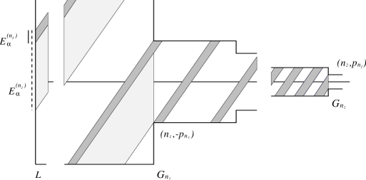
Figure 7: In order to have no escape orbits, $E_{\alpha}^{(n_{1})}$, $E_{\alpha}^{(n_{2})}$, etc. must have upper (equivalently right) extremes in common. This implies that the beams of orbits departing from them have upper boundaries in common, whence the existence of pieces of generalized diagonal. An analysis of the directions $\alpha$ for which this should happen shows that this is not the case (Proposition 6).

Proof. From the previous lemmas, there may be zero escape orbits only for those $\alpha$’s such that there is a sequence $\{n_{j}\}$ with $n.i.(E_{\alpha}^{(n_{j})})=1$. Moreover, in order to have no escape orbits, the intervals $E_{\alpha}^{(n_{j})}$ must eventually share their right extemes. This implies that $\gamma_{n_{j}}$ connects the vertex $V_{n_{j}}$ to the “upper copy” of $V_{n_{j+1}}$, as illustrated in Fig. 7. Note that if $n_{j+1}-n_{j}=1$ for some $j\geq 0$, then $\gamma_{j}$ is an escape orbit (essentially the case (a) of Lemma 7). We can assume that $n_{0}=0$, otherwise can always rescale the billiard. Thus $\gamma_{0}$ connects the vertices $V_{0}$ to $V_{n_{1}}$. By looking at (24)-(24), this happens if, and only if,

$$\alpha=\frac{1}{2}+\frac{1}{n_{1}2^{n_{1}}}+2k_{1}\ \ {\rm or}\ \ \alpha=1+\frac{1}{n_{1}2^{n_{1}}}+2k_{1},$$ (39)

for some integer $k_{1}$. Now, let us consider $\gamma_{1}$. If we rescale vertically the billiard by a factor $2^{n_{1}}$, we get the same setting we had for $\gamma_{0}$. Since $\gamma_{1}$connects $V_{n_{1}}$ to $V_{n_{2}}$, we must have, for some $k_{2}$,

$$2^{n_{1}}\alpha=\frac{1}{2}+\frac{1}{(n_{2}-n_{1})2^{n_{2}}}+2k_{2}\ \ {\rm or}\ \ 2^{n_{1}}\alpha=1+\frac{1}{(n_{2}-n_{1})2^{n_{2}}}+2k_{2}.$$ (40)

Since $n_{2}-n_{1}>1$ and $n_{1}>1$, a comparison between (39) and (40) shows that $1/n_{1}$ must equal $1/2+1/((n_{1}-n_{2})2^{n_{2}})$ or $1+1/((n_{1}-n_{2})2^{n_{2}})$. It is not hard to see that this cannot be the case. Therefore there are no $\alpha$’s such that $\gamma_{0}$ intersects $V_{n_{1}}$ and $V_{n_{2}}$ at the same time. This proves the statement. Q.E.D.

Lemma 6, Lemma 7 and Proposition 6, can be summarized into the following theorem.

Theorem 2

With reference to the step billiard $\Omega$: If there exists a non-negative integer $m$ such that $2^{m}\alpha=4/3\ ({\rm mod}\ 2)$, then there are two escape orbit; otherwise there is only one escape orbit.

We osberve that, if there are two escape orbits, they are distinct even in $\Omega$, by using the same considerations as in the proof of Lemma 2. The core of the theorem, however, is re-expressed in the following important corollary.

Corollary 4

For all but countably many $\alpha>0$ the step billiard has exactly one escape orbit.

2.2 The backward part of an escape orbit

In this section we explore the behavior of an escape orbit for negative times. This question turns out to be crucial for the understanding of the dynamics on the exponential step billiard, as it will explained in Section 3.

As trivial as it is, we point out that the backward part of any escape orbit cannot be periodic; nor it can be bounded, by Proposition 4. What about the possibility for it to escape to $\infty$ as well, having a constant negative $X$-velocity for $t\in]-\infty,t_{0}[$?

Lemma 8

For a.e. $\alpha$, the backward part of an escape orbit does not intersect any vertex.

Proof. Fix an $\alpha$ for which the assertion does not hold: we then have in $R_{\alpha}$ an escape orbit containing a vertex $V$ before it “takes off” towards infinity. $V$ can only be $(0,0)$ or of the form $(p,\pm 2^{-q})$ (incidentally, Fig. 2 shows that $q=|p|$ or $q=|p|+1$).

Let us call $(0,Y_{0})$ the last (in time) intersection point between the orbit and $L$. The geometry of $R_{\alpha}$ implies that

$$Y_{0}=m_{0}2^{-q}+\sum_{i=1}^{j}(\alpha-m_{i}2^{-q_{i}});$$ (41)

with $m_{i},q_{i}\geq 0$ some integers ($m_{0}=0$ or $\pm 1$ depending on $V$ being the origin or not). The above formula is easily understood thinking that $j$ is the number of rectangular boxes visited by the orbit before reaching $L$ for the last time: in each box the variation of the $Y$-coordinate is $\alpha\ ({\rm mod}\ {2^{-q_{i}}})$. We turn now to the rescaled coordinates: $y_{0}=Y_{0}/2$. Thus, rearranging the previous equality yields, for some integers $m,k$,

$$y_{0}=m2^{-k}+\frac{j}{2}\alpha.$$ (42)

Since the orbit is supposed to escape after leaving $(0,Y_{0})$, we can apply (11), (12) with $y_{0}$ as in (42). If $n\geq k$ the first term in (42) gets canceled. Therefore one must have

$$y_{n+1}=(n+j+1)2^{n}\alpha\ ({\rm mod}\ 2)\in\left[-\frac{1}{2},\frac{1}{2}\right[\ \ \ \forall n\geq k.$$ (43)

Consider the increasing sequence $\{n_{i}\}_{i\geq p}$ such that $n_{i}+j+1=2^{i}$ with $n_{p}\geq k$. Condition (43) implies in particular that

$$y_{n_{i}+1}=2^{i+n_{i}}\alpha\ ({\rm mod}\ 2)\in\left[-\frac{1}{2},\frac{1}{2}\right[\ \ \ \forall i\geq p.$$ (44)

By looking at the appendix—especially at Lemma 10—one easily sees that (44) is equivalent to saying that the $-(i+n_{i}+1)$-th digit of the binary expansion of $\alpha$ is a zero for every $i\geq p$. The Lebesgue measure makes these events independent and equally likely with probability $1/2$. Hence (44) can only occur for a null-measure set of $\alpha$’s. This proves that for almost no $\alpha$’s an escape orbit can start from vertex $V$ and pass through $j$ boxes before taking off to infinity. Since events like this are countably many, we see that an escape orbit can almost never leave from a vertex . Q.E.D.

Let us call $D_{1}$ and $D_{2}$ the sets of directions that satisfy, respectively, Corollary 3 and Lemma 8. So $D:=D_{1}\cap D_{2}$ is the “full-measure” set of directions that have all the generic properties we have analyzed so far.

Corollary 5

For a.a. $\alpha$’s, the billiard flow $\phi_{\alpha}^{t}$ over $R_{\alpha}$ around the escape orbit $\eta_{\alpha}$ is a local isometry. This means that, fixed a $z_{0}\in\eta_{\alpha}$, then $\forall T>0,\ \exists\varepsilon>0$ s.t.

$$|z-z_{0}|\leq\varepsilon\Longrightarrow|\phi_{\alpha}^{t}(z)-\phi_{\alpha}^{t}(z_{0})|=|z-z_{0}|\ \ \ \forall t\in[-T/2,T/2].$$

Proof. Since the billiard flow over $R_{\alpha}$ is isometric far from the singular vertices, it suffices to observe that, for $\alpha\in D$, $\eta_{\alpha}$ does not intersect any vertices. As regards the backward part, this is an immediate consequence of Lemma 8 (since $\alpha\in D_{2}$). The same holds for the escaping part, because a singular escape orbit would imply $n.i.(E_{\alpha}^{(n)})=2$ for $n$ large, and this cannot occur for $\alpha\in D_{1}$. Q.E.D.

We recall Leontovich’s notation “oscillating”, as introduced in Section 2.

Theorem 3

For almost all $\alpha$’s, the unique escape orbit is oscillating in the past.

Proof of Theorem 3. Let us take $\alpha\in D$, again, and consider the unique escape orbit $\eta_{\alpha}$. Lemma 8 states that it is non-singular, so the symmetry arguments outlined in the remark in Section 2 apply. Suppose now that $\eta_{\alpha}^{-}$, some past semi-trajectory of $\eta_{\alpha}$, escapes: this corresponds, by reflection, to a forward escape semi-orbit. Then the uniqueness hypothesis shows that the reflected image of $\eta_{\alpha}^{-}$ must coincide with some $\eta_{\alpha}^{+}$. In other words $\eta_{\alpha}$ is symmetric around the origin in $R_{\alpha}$, which means that in $\Omega$ it is run over twice, once for each direction. The situation is illustrated, for both $\Omega$ and $R_{\alpha}$, in Fig. 8. One gets easily convinced that the only way to realize this case is that the trajectory has a point in which the velocity is inverted. This can only be a non-singular vertex. But $\alpha\in D_{2}$ and Lemma 8 claims that this is impossible. Q.E.D.

3 Dynamics on the Billiard

Throughout this section we fix a direction $\alpha\in D$. As defined in Section 2.2, this is the set of directions satisfying all the generic properties which we have explored so far. Hence, for simplicity, we drop the subscript $\alpha$ from all the notation. For example, the unique escape orbit will only be denoted by $\eta$. On it, we fix the standard initial condition $z_{0}=(0,Y_{0})$ as the last intersection point with $L$, before the orbit escapes towards $\infty$.

Rather unexpectedly, it turns out that the statements in Section 2.1, mainly intended to analyze the escape orbits, provide, as a by-product, a certain amount of information about the topology of the flow $\phi^{t}$ on the billiard. Information which, although certainly incomplete, we believe was not a priori obvious. The crucial fact, as it will be noticed, is Corollary 3, which roughly states that not only there is just one initial point that takes a trajectory to infinity, but also there is just one neighborhood—necessarily around that point—that takes a trajectory far enough. This is the idea behind next result.

Lemma 9

Let $\alpha\in D$. Taken an orbit $\gamma$, two numbers $\varepsilon,T>0$, there exists a $w\in\gamma\cap L$, such that

$$|\phi^{t}(w)-\phi^{t}(z_{0})|=|w-z_{0}|\leq\varepsilon\ \ \ \forall t\in[-T/2,T/2],$$

where $z_{0}$ is the standard initial condition on $\eta$. Furthermore, if $\gamma\neq\eta$, $w$ can be chosen arbitrarily far in the past or in the future of $\gamma$. For $\gamma=\eta$, $w$ can be chosen arbitrarily far in the past.

Proof. Since $\alpha$ is typical, we can apply Corollary 5 with $z_{0}$ fixed as above. This will return an $\varepsilon^{\prime}$ (depending on $T$) such that all points as close to $z_{0}$ as $\varepsilon^{\prime}$ remain such under the flow, within a time $T$. Assume $\varepsilon^{\prime}\leq\varepsilon$ (if not, $\varepsilon^{\prime}:=\varepsilon$ will do). We need to find a point of $\gamma$ in the interval $[Y_{0}-\varepsilon^{\prime},Y_{0}+\varepsilon^{\prime}]\subseteq L$. Recalling Corollary 3, consider the subsequence $\{G_{n_{j}}\}$ of apertures whose backward beam of trajectories does not split at any vertex before reaching $L$. Take a $j$ such that $2p_{n_{j}}=2^{-n_{j}+1}\leq\varepsilon^{\prime}$. Since $\gamma$ is unbounded, we can find a point $u\in\gamma\cap G_{n_{j}}$. Call $w$ the last intersection point of $\gamma$ with $L$, before $u$ is reached. From the non-splitting property of $G_{n_{j}}$, $|w-z_{0}|\leq\varepsilon^{\prime}$. Corollary 5 shows that this is the sought $w$.

Proposition 4 actually states that each semi-trajectory of $\gamma\neq\eta$ is oscillating: therefore $u$ (and so $w$) can be chosen with as much freedom as claimed in the last statement of the lemma. As for $\eta$, only the backward part oscillates (Theorem 3). Q.E.D.

Remark. We stress once again that the above is more than an easy corollary of Proposition 3: not only $\gamma$ and $\eta$ get close near infinity, being both squeezed inside the narrow “cusp”, but, to be so, they must have already been as close for a long time.

A number of trivially checkable consequences of Lemma 9 are listed in the sequel. Recall the definitions of $\omega$-limit and $\alpha$-limit of an orbit as the sets of its accumulation points in the future and in the past, respectively (see, e.g. [W], Definition 5.4).

Corollary 6

With the same assumptions and notation as above,

• The escape orbit $\eta$ is contained in the $\omega$-limit and in the $\alpha$-limit of every other orbit.

• The escape orbit $\eta$ is contained in its own $\alpha$-limit.

• Every invariant continuous function is constant.

• The flow is minimal if, and only if, the escape orbit is dense.

Of course, one would like to prove one definite topological property of the flow $\phi^{t}$, such as minimality or at least topological transitivity. Our techniques do not seem to do this job. However, they do furnish a picture of how chaotic the motion on the billiard can be. In fact, the attractor that $\eta$ has been proven to be is certainly far from simple. Either it densely fills the whole invariant surface $R_{\alpha}$, or it is a fractal set.

Theorem 4

For a typical direction ($\alpha\in D$) consider the corresponding flow on $R_{\alpha}$. Denote $L_{\eta}:=\eta\cap L$, the “trace” of the escape orbit with the usual Poincaré section. Then its closure in $L$ (denoted by $\overline{L_{\gamma}}$) is either the entire $L$ or a Cantor set.

Proof of Theorem 4. Assume $\overline{L_{\gamma}}\neq L$. This set is closed. We are going to show it also has empty interior and no isolated points, that is, it is Cantor. In the remainder, by interval we will always mean a segment of $L$.

Suppose the interior of our set is not empty. Then there exists an open interval $I\subseteq\overline{L_{\gamma}}$ containing a point $z$ of $\eta$. Now, in the complementary set of $\overline{L_{\gamma}}$, select a point $w$ whose orbit is non-singular. Let $w$ evolve, e.g., in the future. By Corollary 6,(i) applied to $z$, there is a $t>0$ such that $\phi^{t}(w)\in I$. By the choice of $w$, we can find an open interval $J$, such that $w\in J$, $J\cap\overline{L_{\gamma}}=\emptyset$ and so small that $\phi^{t}$ maps $J$ isometrically into $I$. This implies that $J\subset\overline{L_{\gamma}}$, which is a contradiction.

To show that there are no isolated points: if $z\in\overline{L_{\gamma}}\setminus L_{\gamma}$, there is nothing to prove; if $z\in L_{\gamma}$, then Corollary 6,(ii) does the job. Q.E.D.

4 Conclusions

Although we think we have given a pretty good description of the escape orbits for our model, the exponential step billiard, and we have concluded that those objects are central for the dynamics, the results contained in this paper certainly lack completeness. Even conceding on semiclassical quantum mechanics, one is not satisfied from the point of view of ergodic theory, either. Recalling Theorem 4, we do believe that the flow should be minimal for a.e. $\alpha$, making the Cantor set case an interesting exception. But this does not seem to be easily provable with our techniques, which, we readily admit, use the results for finite polygonal billiards (see Propositions 1 and 2) blindly, without trying to extend them to our case. Most likely, doing so will provide a key to more complete statements.

However, there is already something more to say on the escape orbits for other models of infinite step billiards. Giving up the sharpness of the statements in Section 2.1, strictly designed for the case $p_{n}=2^{-n}$, a result similar to Theorem 2 is at present available for a variety of cases. This is based on some elementary measure-theory and has the advantage that it does not require the exact knowledge of the behavior of the singular semi-orbits $\gamma_{p}$ as a function of $\alpha$ [as in (31)-(31)]. We refer the interested reader to [DDL].

5 Acknowledgments

The authors wish to thank S. De Bièvre, S. Graffi and Ya. G. Sinai for stimulating discussions. Also, M.L. would like to express his gratitude to Ya. G. Sinai for his guidance during these years at Princeton University. The same author has been partially supported by the I.N.F.N. (Gruppo IV, Bologna).

Appendix A Appendix:
The Binary Expansion of a Number

Let $y$ be a real number. Suppose we want to analyze its binary expansion: there exist an $m\in{{Z}}$ such that

$$y=\pm\sum_{j=m}^{-\infty}y^{(j)}2^{-j}=:y^{(m)}\ldots y^{(0)}.y^{(-1)}y^{(-2)}\ldots;$$ (45)

$y^{(j)}=0$ or $1$. In order for this expansion to be in a one-to-one correspondence with ${{R}}$, we adopt the following convention: when $y>0$ all endless sequences of the type $0111111\ldots$ are replaced by $1000000\ldots$; if $y<0$ the rule is inverted. So, for instance, $1/2=0.100\ldots$ and $-1/2=-0.0111\ldots$

The above convention ensures that numbers in $[-1,1[$ are described with no need of integer digits, i.e. $y^{(j)}=0,\,\forall j\geq 0$. Recall that $y\ ({\rm mod}\ 2)$ means the unique real number in $[-1,1[$ congruent to $y$ modulo $2$.

Lemma 10

Let $y\in{{R}}$ and $\{y^{(j)}\}_{j\leq m}$ its binary expansion as in (45). Then $2^{k}y\in[-1/2,1/2[$ if, and only if, $y^{(-k-1)}=0$.

The trivial proof is omitted.

Figures

Figure 1: The infinite billiard table $\Omega$.

Figure 2: The invariant surface $R_{\alpha}$ for the infinite billiard.

Figure 3: The invariant surface $R_{\alpha}^{(n)}$ for the truncated billiard.

Figure 5: Range of directions for which the orbit starting from the leftmost bottom vertex reaches directly aperture $G_{n}$ (case $n=2$ is displayed). The billiard $\Omega$ has been unfolded on the plane, that is, many copies of it are sketched, in order to draw trajectories as straight lines. Considering $\alpha\ ({\rm mod}\ 2)$, for each $n\geq 2$, three beams occur. Fixing one beam relative to $G_{n}$, the geometry of the billiard implies that one, and only one, sub-beam will also reach $G_{n+1}$. Eventually, for $n\to\ +\infty$, these three beams narrow down to the values $\alpha=1/2,1,3/2$, the last of which is rejected for our convention on the continuation of singular orbits.

Figure 6: The structure of the sets $A_{n}$, as in the proof of Lemma 7: $A=\bigcap_{n\geq 0}A_{n}$ consists of two points, both limit of a sequence of nested intervals.

Figure 8: A trajectory can be run over twice only if it contains a non-singular vertex. For a.a. $\alpha$’s this is the only possibility to have an orbit which escapes both in the past and in the future.

References

- [AG] S.H.Aranson and V.Z.Grines, On some invariants of dynamical systems on two-dimensional manifolds (necessary and sufficient conditions for the topological equivalence of transitive dynamical systems), Math. USSR Sbornik 19 (1973), 365-393
- [Ar] P. Arnoux, Ergodicité generique des billards polygonaux, Selinaire Bourbaki 696 (1988), 203-221
- [BKM] C.Boldrighini, M.Keane and F.Marchetti, Billiards in polygons, Ann. Prob. 6 (1978), 532-540
- [B] M.Boshernitzan, Billiards and rational periodic directions in polygons, Amer. Math. Monthly 99 (1992) 522-529
- [CFS] I.P.Cornfeld, S.V.Fomin and Ya.G.Sinai, Ergodic theory, Springer-Verlag, Berlin, 1982
- [DDL] M.Degli Esposti, G.Del Magno and M.Lenci, Infinite Step Billiards II, in preparation
- [FK] R.H.Fox and R.B.Kershner, Concerning the transitive properties of geodesic on a rational polyhedron, Duke Math. J. 2 (1936) 147-150
- [G1] E.Gutkin, Billiard flows on almost integrable polyhedral surfaces, Ergod. Th. & Dyn. Sys. 4 (1984) 569-584
- [G2] E.Gutkin, Billiards in polygons, Physica D 19 (1986) 311-333
- [G3] E.Gutkin, Billiards in polygons: survey of recent results, preprint (1996)
- [GK] E.Gutkin and A. Katok, Weakly mixing billiards, Holomorphic Dynamics, LNM 1345, Springer-Verlag, Berlin (1989)
- [GKT] G.Galperin, T.Krüger and S.Troubetzkoy, Local instability of orbits in polygonal and polyhedral billiards, Comm. Math. Phys. 169 (1995) 463-473
- [Gu] M.C.Gutzwiller Chaos in Classical and Quantum Mechanics Springer-Verlag, New York, 1990
- [KMS] S.Kerckhoff, H.Masur and J.Smillie, Ergodicity of billiard flows and quadratic differentials, Ann. Math. 124 (1986) 293-311
- [K] M.Keane Interval exchange transformations Math. Z. 141 (1975) 25-31
- [Ka] A. Katok Interval exchange transformations and some special flows are not mixing, Israel J. Math. 35 (1980) 301-310
- [Le] M.Lenci, Escape orbits for non-compact flat billiards, Chaos 6,3 (1996) 428-431
- [L] A.M.Leontovich, The Existence of Unbounded Oscillating Trajectories in a Problem of Billiards, Sov. Acad. Sci., doklady Math. 3,4 (1962) 1049-1052
- [M] H.Masur, Interval exchange transformations and measured foliations, Ann. Math. 115 (1982) 169-200
- [V1] W.A.Veech, Interval exchange transformations, J. D’Analyse Math. 33 (1978) 222-272
- [V2] W.A.Veech, Gauss measures for transformations on the space of interval exchange maps, Ann. Math. 115 (1982) 201-242
- [W] P.Walters, An introduction to ergodic theory, Springer-Verlag, GTM 79, New York, 1982
- [ZK] A.Zemlyakov and A.Katok, Topological transitivity of billiards in polygons, Math. Notes 18,2 (1975) 760-764