Front dynamics in turbulent media

Abstract

A study of a stable front propagating in a turbulent medium is presented. The front is generated through a reaction-diffusion equation, and the turbulent medium is statistically modeled using a Langevin equation. Numerical simulations indicate the presence of two different dynamical regimes. These regimes appear when the turbulent flow either wrinkles a still rather sharp propagating interfase or broadens it. Specific dependences of the propagating velocities on stirring intensities appropriate to each case are found and fitted when possible according to theoretically predicted laws. Different turbulent spectra are considered.

I Introduction

Front propagation has been a problem of great interest in a rich variety of nonequilibrium phenomena originating pattern structures [1, 2, 3]. The most usual and studied situation corresponds to a stable (planar) front propagating in a quiescent homogeneous and isotropic medium at a constant velocity. This situation can be modeled easily by a reaction-diffusion equation for the order parameter. Reaction (nonlinear) terms have to present at least two possible steady states: one stable and a second unstable or metastable. Then the stable state propagates through the unstable one. The region where the variable changes abruptly from one state to the other is called the interface or front width, whose size is controlled by the diffusion coefficient. These fronts propagate at a velocity $v_{0}$ which results from the interplay between the chemical time scale (reaction) $\tau_{\rm chem}$ and the species diffusivity coefficient (diffusion) $D$: $v_{0}\sim(D\tau^{-1}_{\rm chem})^{1/2}$. These facts are well known and have been discussed and applied in different fields.

A more complicated situation is found when considering front–like patterns propagating in non–quiescent media. In such a case, the additional length and time scales introduced by the advecting flow will interact with those intrinsic to the reaction-diffusion front dynamics, resulting in new and distinctive propagation regimes. Particularly interesting in this context is the problem of reaction propagation in premixed combustible gases [4]. Mainly due to its practical relevance in combustion processes, the subject has motivated numerous theoretical as well as experimental efforts [5, 6, 7, 8, 9, 10]. The generic understanding coming from these studies is that the turbulent front velocity $v_{T}$ is larger than $v_{0}$, to an extent which depends on the intensity and spatiotemporal correlations of the turbulent flow. Some other issues, however, such as velocity quenching effects, role of turbulent spectra remain somewhat more open.

An enlarged perspective has been gained recently when experiments on liquid phase reactions [11] have brought out a more simplified scenario as compared to that of combustion processes. In such liquid reactions the change of density and the increasing of the temperature are negligible compared with those occurring in typical combustion processes [12]. In this way experimentalists are closer to reproduce the set of simplified assumptions invoked by most of the theoretical models.

An even more controlled situation concerning liquid phase reactions can be envisaged when considering front propagation under externally imposed stirring conditions. This is precisely the context we will address in this paper. In essence, stirring can be thought of as a sort of controlled way to inject energy into a fluid medium through random forces of statistical nature [13, 14]. Especially suited to reproduce such an scenario are the generically called [15] synthetic turbulence generating models. In particular we will employ here an algorithm to generate stochastic, turbulent-like, flows satisfying Langevin type equations [16]. Specifically, random flows with zero mean velocity and statistically isotropic, homogeneous and stationary are created independently of the front conditions.

The closest experimental reference we are aware concerning this question is the recently reported experimental work by Ronney et al. [12] dealing with different stirred media. From the theoretical side however there is no specific literature focusing on stirring effects, so we rely on the general references of front propagation under turbulent flows. Most of the existing theoretical models refer to the so-called Huygens mechanism valid for thin front conditions (“flamelet regime”). Among them we mention those based on the so-called G-equation [7], nonlinear averaging of reaction-diffusion equations [9], and specially, for the purpose of comparison with our results here, the approaches of Kernstein [8], Yakhot [17] and Pocheau [10]. These authors based on different assumptions proposed scaling relations for $v_{T}$ in terms of the intensity of the flow $u_{0}^{2}$. Using the so–called flame propagation equation, a variant of the well-known KPZ-equation, Kernstein and Ashurst [8] obtained a relation valid for weak stirring intensities and large correlation times of the flow. Applying renormalization procedures to the G-equation, Yakhot [17] found a relation without adjustable parameters. Pocheau claimed that both Kernstein and Yakhot laws converge into a quadratic relation when invariance over all the scales is assumed [10].

On the other hand, when relying on computer simulations [18], numerical accuracy and finite size effects commonly restricts the examined scenarios to small turbulent intensities. It is also worth mentioning here the alternative stochastic method reviewed by Pope [5]. In such a formulation, a probability density functional is introduced and, after invoking some closure approximation and elimination of variables procedure, a tractable set of partial differential equations is obtained. The most important difficulties of this method remain at the fundamental level of the closure approximation.

In comparison with these generic procedures, what we gain with our random flow generating algorithm is an easy control over the most representative statistical quantities of the advecting flow: its energy spectrum and spatiotemporal correlations. This in turn enables us to explore the role of these parameters in determining the different propagation regimes and particularly in the enhancement of the front speed under turbulent conditions. In particular, the two basic experimentally identified modes of front propagation under stirring [12], i.e. the previously mentioned Huygens propagation mode and the distributed reaction zone regime, are qualitatively identified and quantitatively analyzed in our simulations. Moreover we are able to explore for each regime the role of a pair of different energy spectra displaying a quite different range of energy containing modes.

The paper is organized as follows. In the next section we summarize the method to simulate the turbulent medium. In Sec. III we introduce the theoretical model of front propagation. Numerical results are presented and commented according the existing theoretical predictions. We devote Sec. IV to draw some conclusions and perspectives.

II Turbulent media modelization

Here we will present a brief summary of the theoretical scheme to simulate a statistically homogeneous, stationary and isotropic turbulent flow characterized by its energy spectrum. As we want to study fronts dynamics under different turbulent conditions we will generate two types of spectra.

As a first example we adopt the Kraichnan’s (K) spectrum [19], describing a distributed band of excitations around a well pronounced peak centered at some well-defined wave number $k_{0}$,

$$E(k)\propto k^{3}\exp\left[-{\frac{3k^{2}}{{2k_{0}^{2}}}}\right].$$ (1)

In order to take into account the influence of a broader spectrum of modes we will modelize another type of turbulent medium with the choice of the Kárman-Obukhov’s (KO) spectrum which was introduced [20] to study Kolgomorov turbulence. To this end we select from the family of KO spectra, the following form:

$$E(k)\propto k^{3}\left[1+{9k^{2}\over{5k_{0}^{2}}}\right]^{-7/3}$$ (2)

which has its maximum also at $k_{0}$.

As we will assume that the characteristics of the flow are not going to be affected by front dynamics, then our method will simply reproduce the above mentioned spectra in a statistical way (see Ref. [16] for more theoretical details).

Our starting point is a generalized Ornstein-Uhlenbeck like Langevin equation for the stream function $\eta({\bf r},t)$,

$${\frac{\partial\eta({\bf r},t)}{{\partial t}}}=\nu\nabla^{2}\eta({\bf r},t)+Q[\lambda^{2}\nabla^{2}]\nabla.\mbox{\boldmath$\zeta$}({\bf r},t)$$ (3)

where $\nu$ is the kinematic viscosity and $\mbox{\boldmath$\zeta$}({\bf r},t)$ is a Gaussian white noise process of zero mean and correlation

$$\left\langle\zeta^{i}({\bf r}_{1},t_{1})\zeta^{j}({\bf r}_{2},t_{2})\right\rangle=2\epsilon_{0}\nu\delta(t_{1}-t_{2})\delta({\bf r}_{1}-{\bf r}_{2})\delta^{ij}.$$ (4)

According to these definitions, $\epsilon_{0}$ and $\lambda$ are control parameters respectively related to the intensity and characteristic length of the random flow. $Q[\lambda^{2}\nabla^{2}]$ plays a relevant role in our approach because it introduces through the random stirring forces the spectra we want to use in each particular case. In particular for the K spectrum we take

$$Q[\lambda^{2}\nabla^{2}]=\exp\left({\frac{\lambda^{2}\nabla^{2}}{{2}}}\right)$$ (5)

where $\lambda=(3/2)^{1/2}k_{0}^{-1}$. On the other hand, the KO spectrum is reproduced through

$$Q[\lambda^{2}\nabla^{2}]=\left(1-\lambda^{2}\nabla^{2}\right)^{-7/6}$$ (6)

where $\lambda=(9/5)^{1/2}k_{0}^{-1}$.

From the stream function, the 2-d incompressible advecting flow is obtained as usual,

$${\bf v}({\bf r},t)=\left(-{\frac{{\partial\eta({\bf r},t)}}{{\partial y}}},{\frac{{\ \partial\eta({\bf r},t)}}{{\ \partial x}}}\right).$$ (7)

This two dimensional version of our algorithm is chosen for the simplicity in dealing with the numerical simulations, but at the same time expresses our belief that the basic trends of front propagation in turbulent media, that we want to analyze here, are well reproduced in this reduced dimensionality. Moreover, recent experiments in chemical reactions in quasi 2-d geometries [12] and theoretical analysis [10] support also this assumption.

The energy spectrum $E(k)$ can be expressed in terms of the Fourier transformed operator $Q(-\lambda^{2}k^{2})$,

$$E(k)={\epsilon_{0}\over{4\pi}}k^{3}Q^{2}(-\lambda^{2}k^{2}).$$ (8)

The stirring intensity, $u_{0}^{2}$, ($u_{0}^{2}=\int_{0}^{\infty}{dkE(k)}$) and integral time $t_{0}$ and length $l_{0}$ scales of the random flows are easily expressed in terms of the functional and parametric specifications for the noise terms left in (3) and (4).

In particular for the K spectrum, we have

$$u_{0}^{2}=\frac{\epsilon_{0}}{8\pi\lambda^{4}};\,\,\,\,\,t_{0}=\frac{\lambda^{2}}{\nu};\,\,\,\,\,l_{0}=\frac{\lambda\sqrt{\pi}}{2}.$$ (9)

And for KO spectrum, we get for the three basic parameters

$$u_{0}^{2}=\frac{9\epsilon_{0}}{32\pi\lambda^{4}};\,\,\,\,\,t_{0}=\frac{\lambda^{2}}{3\nu};$$ (10)

$$l_{0}=\lambda{\Gamma(1/2)\Gamma(5/6)\over{2\Gamma(1/3)}}.$$ (11)

In Fig. 1 three different spectra with the same intensity (kinetic energy) are presented: one of Kraichnan type (a) and two of the Kárman-Obukhov spectrum b) and c). We see how Kraichnan’ s energy distribution shows a pronounced maximum whereas the other spectra are broader and show much longer tails. Spectra (a) and (c) have the same $k_{0}$, but (a) and (b) have the same $l_{0}$. These facts will be of relevance later on to explain the dynamical properties of a front propagating in random media represented by each one of those spectra.

For the sake of comparison, we have considered two additional and somewhat related, turbulent conditions. The first one, hereafter referred on as frozen stirring, corresponds to a frozen configuration of the random flow generated according the rules above introduced. The second one referred on what follows as periodic flow, represent nothing but a periodic set of fixed eddies. It is constructed from the single mode stream function

$$\eta(x,y)=\eta_{0}\cos(\frac{n\pi x}{N})\cos(\frac{n\pi y}{N}),$$ (12)

representing a periodic array of $n\times n$ eddies, where $N$ is defined from the system size $L$ as, $N=L/\Delta x$ .

A detailed presentation of the way the algorithm just proposed is implemented to simulate turbulent flows can be found in [16].

III Front dynamics

A The model and theoretical basis

In this section we present the model used to reproduce a chemical stable front propagating in random media with prescribed statistical properties.

The basic ingredient is a reaction-diffusion scheme which exhibits two steady states of different stability and connected by a front which otherwise propagates in a stable (planar) way. There are many possible choices in the literature [2, 3] and we will take a very simple one which corresponds to that of a generic reaction-diffusion equation for the scalar field $\psi({\bf r},t)$, used as a relevant variable:

$${\frac{\partial\psi}{{\partial t}}}=D\nabla^{2}\psi+f(\psi)$$ (13)

where the nonlinear function $f(\psi)$ has a minimum of two zeros corresponding to the steady states. In our numerical simulations we have chosen the nonlinear function $f(\psi)=\psi^{2}-\psi^{3}$. In this case a stable planar front propagates the stable state $\psi=1$ (“products”) into the invaded metastable one $\psi=0$ (“reactants”). Two important parameters are the dimensionless propagation rate and front thickness which respectively read:

$$v_{0}=\sqrt{\frac{D}{2}},\,\,\,\,\,\,\,\,\delta_{0}=\sqrt{8D}.$$ (14)

The front profile has then the form,

$$\psi(x,t)=\frac{1}{2}\left(1-\tanh(\frac{x-v_{0}t}{\delta_{0}})\right).$$ (15)

Our numerical results have been checked in relation with different choices of the reaction term. Confirming our belief that within our formulation, this choice should not be a relevant point, we have explicitly considered the case $f(\psi)=\psi(1-\psi)(\psi-0.25)$ and the same quantitative results have been obtained.

A turbulent flow is superposed now through a convective term added to Eq. (13)

$${\frac{\partial\psi}{{\partial t}}}=D\nabla^{2}\psi+\psi^{2}-\psi^{3}-{\bf\nabla}.[{\bf v}({\bf r},t)\psi].$$ (16)

As illustrated in Figs. 2a and 2b, numerical simulations of Eq. (16) above, reproduce two distinct limiting regimes of front propagation. In these two figures the flow pattern is also plotted. Small arrows indicate the local velocity vector of the flow.

In Fig. 2a we see a front in a situation where the typical length scale of the flow $l_{0}$ is larger than the intrinsic one associated to the reaction-diffusion dynamics $\delta_{0}$. It is clear that the mean size of the observed eddies is larger than the front width. Then a distorted front propagates with a larger velocity than in the deterministic case but maintaining a still rather sharp and well defined interface. Such a propagation mechanism is known in the combustion literature as the “thin flame,” “flamelet” or “reaction sheet” regime [12].

The other limit corresponds to a situation for which $l_{0}$ is smaller than $\delta_{0}$. Now the mean size of the eddies are comparable or smaller than the interfacial width. This is the situation in Fig. 2b where the front is broader and more diffused than in the former case. This situation is referred in the literature as a “distributed reaction zone”(DRZ) regime [12]. Also in this case we also observe that the front velocity is larger than in quiescent media.

We want to emphasize at this point that both phenomenologies are well known in experiments dealing with front propagation for isothermal chemical reactions [12].

A specific mechanism of front propagation applies to each one of the previously identified modes. The common rationale behind the “thin flame” mode is based on a HP-like argument: the front has the same local structure as in the planar case with normal velocity given by $v_{0}$, but its length increases due to wrinkling and this results on faster propagation velocities. This can be understood as a geometrical consequence of the propagation of curved interface with a local velocity $v_{0}$ [7]. Denoting respectively by $L_{T}$ and $L_{0}$ the front length and the lateral system size, we have

$$\frac{L_{T}}{L_{0}}=\frac{v_{T}}{v_{0}}\equiv S.$$ (17)

On the other hand if we assume that the effect of the flow velocity in the DRZ regime is completely reproduced by increasing the diffusive transport inside the broadened front then such an effect can be incorporated as a renormalization of the diffusion coefficient. In the DRZ mode we simply adapt the first fundamental result of Eq. 14, to obtain

$$S^{2}=\left(\frac{v_{T}}{v_{0}}\right)^{2}=\left(\frac{D_{T}}{D}\right)$$ (18)

where $D_{T}$ is the effective turbulent diffusion. The next and most involved step consists, however, in using Eqs. (17) and (18) above to make detailed predictions for $v_{T}$, or its dimensionless form $S$, as a function of the stirring intensity $u_{0}$, or its dimensionless value $u_{0}/v_{0}\equiv Q$. Let us discuss on what follows our numerical results for the HP and DRZ regimes.

B Results for HP versus DRZ propagation modes

In Figs. (3)–(5) we present our numerical results corresponding to these two modes of front propagation. If it is not explicitly indicated the turbulent flow is that of K spectrum. On what refers to the HP mode, our first task was to check relation (17). The collected data for the different values of $u_{0}^{2}$ are summarized in Fig. 3. For the sake of comparison, we include in this figure results obtained for the other two additional stirring conditions introduced in Sec. II: the frozen stirring and the periodic flow. According to this figure, the geometric argument leading to (17) seems well-supported by our simulations with the simple exception of those situations involving very intense periodic flows. Actually, under these last conditions the interface is largely perturbed by the presence of overhangs whose dynamics contribute positively to the computed velocity, measured as the time variation of the rate of occupation of the $\psi=1$ state, but negatively to the front length.

In Fig. 4, results for $S(Q)$ are specifically plotted corresponding to three of the previously mentioned stirring modes. Figure 4a shows the simulation results of $S^{2}$ versus $Q^{2}$ for a turbulent flow for two different values of $t_{0}$. The theoretical predictions of Yakhot [17], ($S=\exp(Q^{2}/S^{2})$) and Pocheau ($S^{2}=1+2Q^{2}$) [10] are also plotted. Numerical data of the case of frozen stirring are included for comparison. Actually, the numerical results fit reasonably well the linear relation $S^{2}=1+\alpha Q^{2}$, for the whole range of $Q$. Nevertheless, the slope of such a linear law depends on $t_{0}$, a fact not considered in theoretical predictions of Yakhot and Pocheau. Remarkably, these theoretical predictions fit better with our numerical results for frozen stirring (limit of very large $t_{0}$). This agreement is not surprising because in Pocheau’s analysis, both theoretical and experimental, a very large value of $t_{0}$ was considered [10]. Moreover, for this last flow, the behavior largely depends on the examined range of $Q$: the former behavior transforms into a $S=1+\alpha^{\prime}Q^{\frac{4}{3}}$ when approaching the smallest values of $Q$ here considered (Fig. 4b).

Finally, results for the periodic stirring also show a crossover from a linear dependence at large $Q$ towards the quadratic form: $S^{2}=1+\alpha^{\prime\prime}Q^{2}$ at small $Q$ (Fig. 4c). Results for the last two cases are in agreement with theoretical predictions by Kernstein et al. [8].

A final comment is worth emphasizing at this point: Turbulent propagation velocities fall always lower than those obtained for frozen and periodic stirring. This is somewhat at odds with what is reported in Refs [6, 12], although one should keep in mind that the range of $Q$ values there considered were of two orders of magnitude larger than ours.

In Fig. 5 results for the DRZ regimen are presented. The numerical data obtained under different stirring mechanisms are plotted. These numerical results are compared with the corresponding theoretically predicted values based on Eq. (18) above. The values of the effective diffusion coefficient $D_{T}$ have been obtained independently from direct simulation of pure scalar diffusion (without reaction). Theoretical predictions based in Eq. (18) exhibit a remarkable agreement with numerical results for a broad set of the $Q$ values here considered and irrespective of the type of stirring flow considered. Moreover, the theoretical dependences of $D_{T}$ on $u_{0}^{2}$ either for random flows in the weak stirring limit ($D_{T}-D\sim u_{0}^{2}t_{0}$) [16] or for periodic flows in the limit of small Peclet number ($D_{T}-D\sim u_{0}^{2}/D$) [21], are clearly confirmed in this Fig. 5.

C Results for K versus KO spectra

In order to investigate the influence of the different spectra on the enhancement of the front speed, we present in Fig. 6 numerical results corresponding to the two regimes of front propagation previously identified and the pair of turbulent spectra introduced in Sec. II. Respectively, Fig. 6a reproduces conditions of thin front propagation, whereas Fig. 6b those for distributed reaction fronts. Both in Figs. 6a and 6b, circles stand for results obtained with K spectrum, whereas squares and romboids correspond to the KO distribution. Since both spectra can be compared either on the basis of their integral length scale, $l_{0}$, or of their maximum, $k_{0}$, we have chosen to separately consider both cases. Specifically, squares represent simulations from both spectra with the same value of $l_{0}$, i. e. comparing cases a) and b) in Fig. 1, and romboids correspond to both spectra taken at equal values of $k_{0}$, i.e. comparing cases a) and c) in Fig. 1. On the other hand, black circles in Fig. 6a and black and white ones in Fig. 6b are respectively replotted from Figs. 4a and 5. Just for the sake of comparison, we have also included in Fig. 6a as white circles, results for $S^{2}$ obtained from the simulated values of the effective diffusion through the use of expression (18).

Let us start with the conditions of the HP regime (Fig. 6a). When both spectra are taken at equal $l_{0}$, we find smaller values of the turbulent front velocity for KO than for K spectrum. The situation is just the reverse one when both spectra are taken with the same maximum. Both findings admit a rather direct interpretation. From Fig. 1a we conclude that when both spectra have equal integral length scale, the KO distribution displays its maximum at a smaller value of $k_{0}$. This means that in this last case larger length scale modulations are going to be the most relevant ones in bending the propagating interface. This in turn means that the front length is going to be less enhanced and, since we are referring to the HP propagation mode, so will happen with the effective front speed. Contrarily when the two maxima coincide, what makes the difference is the long tail in the KO distribution. Such large wavenumbers, small spatial modulations, are going to be very effective both in wrinkling more intensively the front interface but even more, by interfering the front dynamics at scales comparable to the front thickness. Both effects lead to larger values of the turbulent front velocity. In particular the last mentioned feature is evidenced when observing that results for the KO spectrum approach in this case those that would correspond to a front subjected to the K distribution and propagating under the enhanced diffusion mechanism (white circles). A somewhat similar enhancement of the front velocity at moderate $Q$ has been found in a theoretical analysis [22] when a thin front is slightly perturbed at scales smaller than $\delta_{0}$.

Let us turn now to the DRZ regime of Fig. 6b. What we observe in this situation is that no appreciable effect is found when both maxima coincide in the respective spectra. However, smaller values of $S^{2}$ are observed for equal integral length scales. Analogously as before, both results can be interpreted just by looking at Fig. 1. In the first case, one can imagine that the interface thickness would be wide enough to comprise the most energetic wavenumbers of both flows in such a way that the effective diffusion would be similarly renormalized. Contrarily when prescribing an equal value of $l_{0}$, those more energetic modes in the KO distribution are shifted to smaller wavenumbers and in turn are going to be less effective in enhancing the effective diffusion.

IV Summary and Perspectives

In summary, we have presented here a simple model of a chemical front propagating in a turbulent media. Although artificial, the model reproduces realistic scenarios of front propagation modes in chemical experiments. The observed dependences of the propagating front velocities on the parameters and characteristics of the flow compares well with some of the most well-known relations proposed in the literature. The simplicity and versatility of the computer implementation of turbulent flows and the simple model used to describe the front propagation in these media open new perspectives in the study of more complicated situations in turbulent fluids.

FIG. 1.: Comparison of Kraichnan (a) and Kárman–Obukhov (b) and (c) spectra. Continuous lines correspond to the analytical expression Eq. (8) and symbols stand for simulation results in the discrete lattice. (a) Kraichnan, $l_{0}=4.0$, $k_{0}=0.27$; (b) and (c) Kárman-Obukhov $l_{0}=4.0$, $k_{0}=0.12$ and $l_{0}=1.85$, $k_{0}=0.27$ respectively. The intensity (kinetic energy) is fixed to $u_{0}^{2}=0.25$. Unless otherwise stated a square lattice of $128$x$128$ points and unit spacing $\Delta=0.5$ has been employed in all our simulations.

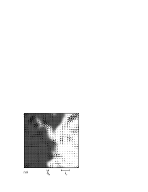
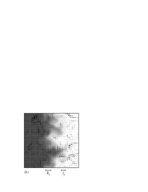
FIG. 2.: Density plot of the stirred reaction front for the K spectrum. The arrows stand for the local velocity field plotted every $4$ mesh points in each direction. (a) corresponds to the thin front mode, parameter values are $D=0.3$, $u_{0}^{2}=3.0$, $\lambda=4.5$ and $t_{0}=1.0$ (b) corresponds to the distributed reaction front regime for $D=2.0$, $u_{0}^{2}=10.0$, $\lambda=2.2$, $t_{0}=1.0$.

FIG. 3.: $S$ vs $L_{T}/L_{0}$ for turbulent flow (circles, $l_{0}=4.0$, $t_{0}=0.1$), random frozen (squares, $l_{0}=4.0$) and periodic eddies (triangles, $8\times 8$ eddies). In all the simulations presented in this figure we have employed $D=0.3$.

FIG. 4.: $S(Q)$ for three stirring modes: turbulent flows (circles, $t_{0}=0.1$; romboids, $t_{0}=3.0$), frozen stirring (squares), and periodic eddies (triangles). The same parameter values of Fig. 3 have been employed. Continuous lines stand for the theoretical predictions (see the text). a): Turbulent and frozen flows. b): Frozen flow and c): Periodic flow.

FIG. 5.: S vs $Q$ for DRZ regime, full symbols denote simulation results of the front propagation while open symbols stand for simulation of the pure effective diffusion Eq. 18 (without reaction). In all the simulations we have employed $D=2.0$. Circles, squares and triangles correspond to turbulent flow ($l_{0}=2.0$, $t_{0}=0.1$), frozen stirring ($l_{0}=2.0$) and periodic eddies respectively ($16\times 16$ eddies). Continuous lines stand for theoretical predictions (see text).

FIG. 6.: Comparison between K and KO spectra. Circles stand for the K spectrum while squares and romboids stand for the KO spectrum with the same $l_{0}$ and the same $k_{0}$ respectively (see Fig. 1). Black circles are the same simulation data of Figs. 4a and 5, and white circles correspond to the simulated effective diffusion. (a) Thin front propagating mode. (b) Distributed front propagating mode. For KO spectrum we have employed $N=256$.

- [1] P. Pelcé, Dynamics of Curved Fronts, Persp. in Physics (Academic Press, 1988).
- [2] J.D. Murray, Mathematical Biology (Springer, New York, 1989).
- [3] M.C. Cross and P.C. Hohenberg, “Pattern formation outside equilibrium,” Rev. Mod. Phys. 65, 851 (1993).
- [4] F.A. Williams, Combustion Theory, 2nd ed. (Benjamin-Cummins, Menlo Park, California, 1985).
- [5] S.B. Pope, “Turbulent premixed flames,” Annu. Rev. Fluid Mech. 19, 237 (1987).
- [6] P.D. Ronney, “Some open issues in premixed turbulent combustion,” in Modeling in Combustion Science, J. Buckmaster and T. Takeno Eds, Lectures notes in Physics, vol. 449 (Springer-Verlag, Berlin, 1995).
- [7] A.R. Kernstein, W.T. Ashurst, and F.A. Williams, “Field equation for interface propagation in a unsteady homogeneous flow field,” Phys. Rev. A 37, 2728 (1988). For a recent review see also P.F. Embid, A.J. Majda, and P.E. Souganidis, “Comparison of turbulent flame speeds from complete averaging and the G-equation,” Phys. Fluids 7, 2052 (1995).
- [8] A.R. Kernstein and W.T. Ashurst, “Propagation rate of growing interfaces in stirred fluids,” Phys. Rev. Lett. 68, 934 (1992).
- [9] S.P. Fedotov, “Reaction front propagation in a turbulent flow,” J. Phys. A: Math. Gen. 28, L461 (1995), A.J. Majda and P.E. Souganidis, “Bounds on enhanced turbulent flame speeds for combustion with fractal velocity fields,” J. Stat. Phys. 83, 933 (1996).
- [10] A. Pocheau, “From turbulent flame fronts to their wrinkling process: scale invariance and similarity,” C.R. Acad. Sci. Paris 319, s II, 879 (1994), A. Pocheau and D. Queiros-Condé, “Scale covariance of the wrinkling law of turbulent propagating interfaces,” Phys. Rev. Lett. 76, 3352 (1996).
- [11] S.S. Shy, P.D. Ronney, S.G. Buckley, and V. Yakhot, “Experimental simulation of premixed turbulent combustion using aqueous autocatalytic reactions,” Proceedings of the 24th Symposium (International) on Combustion (Combustion Institute, Pittsburgh, 1992).
- [12] P.D. Ronney, B.D. Haslam, and N.O. Rhys, “Front Propagation rates in randomly stirred media,” Phys. Rev. Lett. 74, 3804 (1995), B.D. Haslam and P.D. Ronney, “Fractal properties of propagating fronts in a strongly stirred fluid,” Phys. Fluids 7, 1931 (1995).
- [13] G.K. Batchelor, The Theory of Homogeneous Turbulence (Cambridge University, Cambridge, 1970).
- [14] W.D. Mc Comb, “Theory of turbulence,” Rep. Prog. Phys. 58, 1117 (1995); W.D. Mc Comb The Physics of Fluid Turbulence (Oxford University, Oxford, 1990).
- [15] A. Juneja, D.P. Lathrop, K.R. Sreenivasan, and G. Stolovitzky, “Synthetic turbulence,” Phys. Rev. E 49, 5179 (1994); M. Holzer and E.D. Siggia, “Turbulent mixing of a passive scalar,” Phys. Fluids 6, 1820 (1994).
- [16] A. Careta, F. Sagués, and J.M. Sancho, “Generation of homogeneous isotropic turbulence with well-defined spectra,” Phys. Rev. E 48, 2279 (1993); A.C. Martí, J.M. Sancho, F. Sagués, and A. Careta “Langevin approach to generate synthetic turbulent flows,” Phys. Fluids, 9, 1078 (1997).
- [17] V. Yakhot, “Propagation velocity of premixed turbulent flames,” Combust. Sci. Tech. 60, 191 (1988).
- [18] D.C. Haworth and T.J. Poinsot, “Numerical simulations of Lewis number effects in turbulent premixed flames,” J. Fluid Mech. 244, 405 (1992).
- [19] R.H. Kraichnan,“Diffusion by a random velocity field,” Phys. Fluids 13, 22 (1970).
- [20] T.V. von Kárman,“Progress in the theoretical theory of turbulence,” Proc. Natl. Acad. Sci. U.S.A. 34, 530 (1948); A.M. Obukhov, “On the distribution of energy in the spectrum of turbulent flow,” C.R. Acad. Sci. USSR 32, 19 (1941).
- [21] H.K. Moffat, “Transport effects associated with turbulence with particular attention to the influence of the helicity,” Rep. Prog. Phys. 46, 621 (1993).
- [22] P.D. Ronney and V. Yakhot, “Flame broadening effects on premixed turbulent flame speeds,” Combust. Sci. and Tech. 86, 31 (1992).