Burridge–Knopoff Models as Elastic Excitable Media

Abstract

We construct a model of an excitable medium with elastic rather than the usual diffusive coupling. We explore the dynamics of elastic excitable media, which we find to be dominated by low dimensional structures, including global oscillations, period-doubled pacemakers, and propagating fronts. We suggest that examples of elastic excitable media are to be found in such diverse physical systems as Burridge–Knopoff models of frictional sliding, electronic transmission lines, and active optical waveguides.

The response to a perturbation is the defining characteristic of an excitable element. Above a certain threshold in amplitude, a perturbation will excite a quiescent element that then decays back to quiescence after a characteristic time insensitive to the magnitude of the perturbation, during which it is unresponsive to further perturbations. Excitable elements, when coupled to their neighbors into an assembly, become an excitable medium. Models of excitable media with diffusive coupling, such as those of van der Pol, FitzHugh, and Nagumo [4] have successfully described pattern formation phenomena in biology and chemistry, and have also captured the attention of many working in the area of nonlinear science because of their complex spatiotemporal dynamics [5]. On the other hand, the properties of excitable media with elastic rather than diffusive coupling have not to date been investigated. We present here some physical systems — frictional sliding, electronic transmission lines, and active optical waveguides — as diverse examples of such elastic excitable media, and analyze their dynamics, which we find to be dominated by low dimensional structures, including global oscillations, period-doubled pacemakers, and propagating fronts. We investigate the stability of the oscillations, and estimate the velocity of the fronts.

Whilst touching on electronic and optical applications of elastic excitable media, we shall concentrate on frictional sliding. The Burridge–Knopoff model [6] was originally introduced as a representation of earthquake fault dynamics. It describes the interaction of two tectonic plates in a geological fault as a chain of blocks elastically coupled together and to one of the plates, and subject to a friction force by the surface of the other plate, such that they perform stick–slip motion. In this Letter, we show that a Burridge–Knopoff model in which the usual Carlson–Langer velocity weakening dry-friction law [7] is replaced by the original Burridge–Knopoff lubricated creep–slip version showing viscous properties at both the low and high velocity limits, is an elastic excitable medium.

The reintroduction of this friction law in the Burridge–Knopoff model is motivated by experiments showing that it represents friction in a range of materials, including paper on paper [8], metal on metal [9], and rock on rock [10], and by theoretical arguments [11]. The model well represents the qualitative characteristics of laboratory stick–slip experiments with elastic gels [12]. Further interest derives from studies of peeling adhesive tape [13], of Saffman–Taylor fracture in viscous fingering [14], and of the Portevin–Le Châtelier effect of discontinuous yielding [15], showing that stick–slip phenomena in those systems are induced by this same form of friction law.

Burridge & Knopoff introduced a class of simple models that describe the contact region between two tectonic plates as a chain of $N$ blocks of equal mass $m$, mutually coupled by springs of Hooke constant $k_{c}$ and equilibrium length $a$. The blocks are pulled by the bulk of one plate moving at velocity $V$ through constant elastic shear $k_{p}$ against the friction $F_{f}$ between the two plates, as shown in Fig. 1(a). In the stationary frame, the equation of motion for the $i$th block is

$$m\ddot{X}_{i}=k_{c}(X_{i+1}-2X_{i}+X_{i-1})$$ (1)

$$\mbox{}-k_{p}(X_{i}-Vt)-F_{f}(\dot{X}_{i}),$$ (2)

where $X_{i}$ is the departure of block $i$ from its equilibrium position. Usually, following Carlson & Langer [7], the friction is taken to be asymptotically velocity weakening, so that the blocks perform stick–slip motion: any individual block sticks to the surface until the pulling force exceeds the static friction threshold. Once the block starts slipping, the dynamic friction diminishes monotonically with its velocity, as Fig. 1(b) illustrates. While this multivalued form of the friction law is perfectly admissible in the discrete model of Eq. (2), it clearly poses a problem if we attempt to take the continuum limit [16].

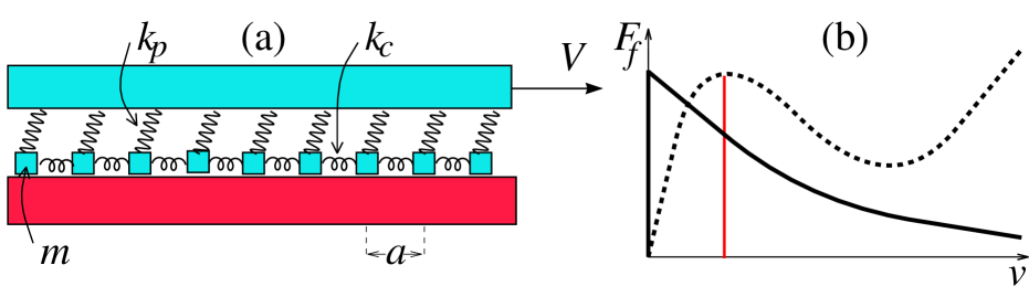
FIG. 1.: (a) The Burridge–Knopoff model. (b) The velocity weakening stick–slip friction law of Carlson & Langer [$F_{f}(v)=F_{0}\,{\mathrm{s}gn}(v)/(1+|v|)$, where $v$ is the velocity of the block] (solid line) and the Burridge–Knopoff type creep–slip friction law we use (dashed line), showing the threshold (vertical line) where the block starts to slip.

To overcome this difficulty, one may replace the static friction discontinuity by a small region of high viscosity. Physically, one can see this cut-off as representing lubrication effects that produce stable creep at low velocities, making our model creep–slip rather than stick–slip. Since we wish to model the frictional characteristics displayed by a range of materials [8, 9, 10], we also have the friction become viscous (velocity strengthening) at high velocities, rather than decay to zero as in the Carlson–Langer version. Our friction model (Fig. 1(b)), which is similar to that originally introduced by Burridge & Knopoff, thus comprises three regions: first velocity strengthening, then velocity weakening, and finally velocity strengthening again. We shall refer to this model as asymptotically velocity strengthening, to be contrasted with the asymptotically velocity weakening friction usually considered. With this in mind, the continuum limit of Eq. (2) in dimensionless variables (see, e.g., [16]) is

$$\ddot{\chi}=c^{2}\chi^{\prime\prime}-(\chi-\nu t)-\gamma\,\phi(\dot{\chi}).$$ (3)

$\chi(x,t)$ represents the time-dependent local longitudinal deformation of the surface of the upper plate in the static reference frame of the lower plate; dots and primes are temporal and spatial derivatives, respectively. In this continuum limit, the number of blocks $N$ becomes the system size $S$. $\phi(\dot{\chi})$ is our normalized asymptotically velocity strengthening friction. There are three dimensionless parameters: $\gamma$ measures the magnitude of the friction, $c$ is the longitudinal speed of sound, and $\nu$ represents the pulling velocity or slip rate. From Eq. (3), we obtain an expression for the local velocity $\psi=\dot{\chi}$ of the interface that, written as a couple of differential equations of first order in time, gives us our continuum Burridge–Knopoff model

$$\dot{\psi} = \gamma(\eta-\phi(\psi)),$$ (5)

$$\dot{\eta} = -\gamma^{-1}(\psi-\nu-c^{2}\psi^{\prime\prime}).$$ (6)

With the proper choice of the function $\phi(\psi)$, and if we may disregard for a moment the positioning of the spatial derivatives term, Eqs. (Burridge–Knopoff Models as Elastic Excitable Media) constitute a version [17] of the van der Pol–FitzHugh–Nagumo model that is the prototypical description of an excitable medium.

While this type of medium was first studied in the physiology of cardiac and nervous tissues, the same properties are also seen in chemical and physical systems. An electrical caricature of an element of an excitable biological membrane is given by the circuit shown in Fig. 2(a). The membrane represented by the capacitor $C$ is charged by ion pumps characterized by the current generator $i_{0}$ and drained through a nonlinear resistance $n_{l}$ across the membrane. This nonlinear element should have the $v-i$ characteristic $\phi$ shown in Fig. 2(b), and could be implemented by a tunnel diode, a neon lamp, or any electronic device with a range of negative resistance. The inductance $L$ models the finite switching time of the ion channels in the membrane. The circuit equations are then formally equivalent to Eqs. (Burridge–Knopoff Models as Elastic Excitable Media) above, where $\psi$ and $\eta$ are proportional to the current and potential difference across the nonlinear device, respectively, and the current $i_{0}$ is proportional to $\nu$. Such circuit elements have been used in electronic experiments with Burridge–Knopoff models [18]. In the models of excitable media of FitzHugh & Nagumo, $\phi$ is generally taken to be as in Fig. 2(b): it thus has exactly the same form as used in our Burridge–Knopoff model (cf. Fig. 1(b)).

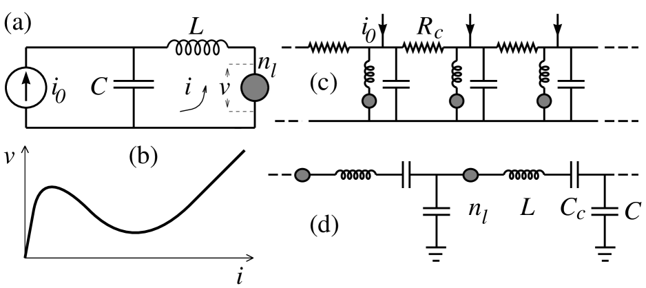
FIG. 2.: An electronic excitable medium. (a) An element of the medium: the circuit and (b) the $v-i$ characteristic of $n_{l}$. (c) Resistive (diffusive) spatial coupling. (d) Capacitive (elastic) spatial coupling — an active transmission line.

The spatial derivatives in Eqs. (Burridge–Knopoff Models as Elastic Excitable Media) are unusual in the realm of excitable media. In a biological excitable membrane, the excitation propagates in space by diffusion. With the electrical model described above one can build a spatially extended diffusive medium by coupling resistively several excitable elements, as indicated in Fig. 2(c). Such a coupling would give rise to current diffusion: the term involving $\psi^{\prime\prime}$ would appear in Eq. (5) instead of in Eq. (6). As they are written however, Eqs. (Burridge–Knopoff Models as Elastic Excitable Media) represent the network of capacitively coupled excitable elements illustrated in Fig. 2(d). This is a discrete representation of an active transmission line, where $L$ and $C$ are the distributed inductance and capacitance and $n_{l}$ is the distributed gain achieved by a nonlinear negative resistance along the line. The distributed serial capacitance $C_{c}$ represents the effects of dispersion in the line. The continuum limit of this network is a caricature of an active optical waveguide such as a fiber amplifier or laser.

Further motivation for the study of Eqs. (Burridge–Knopoff Models as Elastic Excitable Media) is provided by laboratory experiments [12] in which an elastic gel was placed in a Taylor–Couette type apparatus. Stick–slip events occurred at the contact surface of the gel with the rotating inner cylinder. In a large part of the parameter space, low dimensional structures — continuous slip, global oscillations, and propagating fronts — were found rather than complex spatiotemporal patterns that might have been expected to dominate. With this experiment in mind we focus on periodic boundary conditions. Since we are interested in qualitative aspects of the dynamics, we concentrate on the case where $\phi$ is taken to be a cubic polynomial. By shifting the origin of the variables $\psi$ and $\eta$ and the parameter $\nu$ we can reduce $\phi$ to the form $\phi(\psi)=\psi^{3}/3-\psi$. This makes our model a set of elastically coupled van der Pol oscillators. For this election of $\phi$, the slip threshold, defined as the crossover as we increase $\nu$ from velocity strengthening creep to velocity weakening slip, lies at $\nu=-1$.

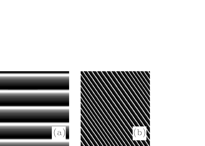
FIG. 3.: Spatiotemporal plots of $\psi(x,t)$ where time is vertical, space is horizontal. (a) A plot of the solution with stable uniform global oscillations for $\nu=-0.92$. (b) Stable propagating fronts at $\nu=-0.96$. In both cases, the other parameter values are $\gamma=2$ and $c=0.3$. The system size $S=20$, and the time elapsed $50$.

The continuous slip solution, where one surface moves uniformly with respect to the other, was examined by Carlson & Langer [16]. They showed that the growth rate of perturbations of any wavelength at a particular slip rate is minus the slope of the friction function at that slip rate. This implies that with asymptotically velocity weakening friction the continuous slip solution is always unstable, while in our case this solution is stable for high and low slip rates where the slope is positive. Global oscillations, where one surface moves periodically in time with respect to the other, are also stable at some slip rates in our model. Figure 3(a) shows the spatiotemporal pattern generated from an arbitrary initial condition with the system relatively far above the slip threshold. Here all points of space oscillate in phase with an instantaneous velocity that follows the dynamics of the van der Pol oscillator. To confirm the stability of these oscillations, we have calculated their Floquet multipliers. Global oscillations are solutions of Eqs. (Burridge–Knopoff Models as Elastic Excitable Media) with the spatial derivative set to zero, which correspond to the period-$T$ limit cycle of the van der Pol oscillator $\vec{\Psi}^{*}(t+T)=\vec{\Psi}^{*}(t)$ where $\vec{\Psi}^{*}(t)=(\psi^{*}(t),\eta^{*}(t))$, which is stable against spatially homogeneous perturbations for $-1<\nu<1$ (i.e., above the slip threshold). We consider small spatial perturbations of the form $\vec{\Psi}^{*}(t)+\vec{\varepsilon}(t)\exp(iqx)$. Dropping quadratic and higher powers of $\vec{\varepsilon}(t)$ in Eqs. (Burridge–Knopoff Models as Elastic Excitable Media), the resulting linear equations for $\vec{\varepsilon}(t)$ have time-periodic coefficients, and by the Floquet theorem their general solution is $\vec{\varepsilon}(t)=\vec{\varepsilon}_{0}P(t)\exp(\Lambda_{q}t)$, where $P(t)$ is a period-$T$ matrix and $\Lambda_{q}$ a time-independent matrix. Once the limit cycle has been numerically determined, the matrix $\exp(\Lambda_{q}T)$ may be computed by numerically integrating the linearized equations over the period $T$. Its two eigenvalues, the Floquet multipliers $(m_{q}^{(1)},m_{q}^{(2)})$, which may be either real, or complex conjugates, determine the stability of global oscillations under perturbations of wavenumber $q$. The growth rate per period of such a perturbation is the maximal Floquet exponent $\lambda_{q}=\max_{i}\{\Re[\ln(m_{q}^{(i)})]\}$. The dispersion relation $\lambda_{q}$ as a function of $q$ relatively far above the slip threshold is never positive, implying stability under perturbations of all scales. This contrasts with the same calculations performed for asymptotically velocity weakening friction, when there is always a range of long wavelengths for which perturbations grow exponentially, so that global oscillations are always unstable when this wavelength is within the system size. This is a significant difference between our model and Burridge–Knopoff models with asymptotically velocity weakening friction. Such global oscillations have been noted in laboratory friction experiments with elastic gels [12].

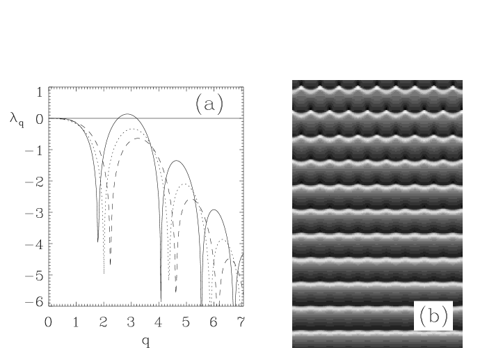
FIG. 4.: (a) A family of dispersion relations for the Floquet exponent showing the destabilization close to the slip threshold of global oscillations against perturbations of a single wavenumber $q_{c}\simeq 3$. Shown are dispersion relations for (from the lower to the upper curve) $\nu=-0.90$, $-0.92$, and $-0.94$. (b) Spatiotemporal plot of $\psi(x,t)$ for $\nu=-0.94$ showing the development of period-doubled structures resulting from this destabilization. Time elapsed is $125$, other settings are as in Fig. 3. The spatial periodicity is determined by $q_{c}$.

For slip rates not far above the slip threshold, global oscillations become unstable. The dispersion relation in Fig. 4(a) shows that the destabilization occurs at a single finite wavenumber $q_{c}$. Furthermore, the Floquet multiplier $m_{q_{c}}$ associated with the maximal Floquet exponent crosses the complex unit circle through $-1$ at this point, indicating a period-doubling bifurcation. Figure 4(b) is a spatiotemporal plot showing the nature of the structure arising near this instability. Small perturbations from the global uniformly oscillating regime grow to become structures with a well-defined wavenumber $q_{c}$. For system size $S$, such structures evolve into a configuration of $q_{c}S/(2\pi)$ synchronized pacemakers emitting fronts in both directions. These fronts annihilate each other at the corresponding $q_{c}S/(2\pi)$ points, that then in turn become pacemakers. The resulting spatiotemporal structure is such that at an arbitrary point in space the periodicity in time is twice that of the original oscillations. These period-doubled structures are not well known in pattern formation, so their presence here is an interesting theoretical prediction.

At slip rates right above the slip threshold, the front solutions cease to annihilate each other and evolve into fronts that propagate right around the system (Fig. 3(b)). One can get an analytical handle on these propagating fronts by positing solutions of the type $\psi(x,t)=f(\tilde{z})$, where $\tilde{z}=x/v+t$, and $v$ is the front velocity. This ansatz with the further rescaling $z=\tilde{z}/\sqrt{1-c^{2}/v^{2}}$ leads to

$$\frac{d^{2}f}{dz^{2}}+\mu(f^{2}-1)\frac{df}{dz}+f=\nu,$$ (7)

which is again the van der Pol equation, but with the nonlinearity rescaled by $\mu=\gamma/\sqrt{1-c^{2}/v^{2}}$. The propagating fronts are then periodic solutions of the van der Pol equation. The parameter $\mu$ is undefined until the value of the front velocity $v$ is chosen. However, we know that the period of the solution is a function $T=T(\mu)$ of $\mu$: in the limit of large $\mu$, $T$ behaves as $T=k\mu+O(\mu^{-1})$, where $k=3+(\nu^{2}-1)\ln[(4-\nu^{2})/(1-\nu^{2})]$ [17]. Since this period should be commensurate with the system size $S$, we have the condition $nT(\mu(v))=S/(v\sqrt{1-c^{2}/v^{2}})$, where $n$ is an integer, to select the allowed front velocities, which in the large $\mu$ limit gives us the quantizing condition $v=S/(nk\gamma)$. Because Eq. (7) has bounded solutions only if $v^{2}>c^{2}$, the propagating fronts are supersonic. Such supersonic propagating fronts have also been noted in Burridge–Knopoff models with asymptotically velocity weakening friction [19, 20].

The original Burridge–Knopoff model was introduced as a means to reproduce the gross features of the statistics of real earthquakes [6]. The Gutenberg–Richter power-law distributions [21] in the statistics of slip events in the model have been considered as an example of self-organized criticality [7], and have been related to the presence of infinitely many degrees of freedom in the system [22]. However, recent numerical experiments [19, 23] indicate that power-law distributions of slip events may be due to discretization, finite size, and transient effects, and are not present at long times in the continuum limit. This has lead to a questioning of the relevance of the model to earthquakes in the real world. Our aim here, however, has been to investigate a Burridge–Knopoff model with a physically interesting friction law relevant to laboratory friction experiments: ours are simply laboratory earthquakes.

We have returned to the asymptotically velocity strengthening type of friction law originally introduced by Burridge & Knopoff, which was abandoned by Carlson & Langer and later investigators, and with it have been successful in explaining some results of laboratory friction experiments. Our model constitutes a form of excitable medium, not previously considered, with elastic instead of diffusive coupling between spatial elements. We have studied the spatiotemporal dynamics of elastic excitable media and find novel dynamics. We believe that this type of elestic excitable medium may have applications beyond laboratory friction experiments to electronic transmission lines and active optical waveguides.

We should like to thank Miguel Angel Rubio and Ed Spiegel for useful discussions. We acknowledge the financial support of the Spanish Dirección General de Investigación Científica y Técnica, contracts PB94-1167 and PB94-1172.

REFERENCES

- [1] julyan@hp1.uib.es, WWW http://formentor.uib.es/julyan.
- [2] dfsehg4@ps.uib.es, WWW http://formentor.uib.es/emilio.
- [3] piro@hp1.uib.es, WWW http://formentor.uib.es/piro.
- [4] B. van der Pol and J. van der Mark, Phil. Mag. 6, 763 (1928); R. FitzHugh, J. Gen. Physiol. 43, 867 (1960); Biophys. J. 1, 445 (1961); J. S. Nagumo, S. Arimoto, and S. Yoshizawa, Proc. IREE Aust. 50, 2061 (1962).
- [5] E. Meron, Phys. Rep. 218, 1 (1992).
- [6] R. Burridge and L. Knopoff, Bull. Seismol. Soc. Am. 57, 341 (1967).
- [7] J. M. Carlson and J. S. Langer, Phys. Rev. Lett. 62, 2632 (1989).
- [8] F. Heslot et al., Phys. Rev. E 49, 4973 (1994).
- [9] Y. Brechet and Y. Estrin, Scripta Metall. 30, 1449 (1994).
- [10] B. D. Kilgore, M. L. Blanpied, and J. H. Dieterich, Geophys. Res. Lett. 20, 903 (1993).
- [11] B. N. J. Persson, Phys. Rev. B 51, 13568 (1995).
- [12] M. A. Rubio and J. Galeano, Phys. Rev. E 50, 1000 (1994).
- [13] D. C. Hong and S. Yue, Phys. Rev. Lett. 74, 254 (1995).
- [14] D. A. Kurtze and D. C. Hong, Phys. Rev. Lett. 71, 847 (1993).
- [15] L. P. Kubin and Y. Estrin, Acta Metall. 33, 397 (1985); M. A. Lebyodkin, Y. Brechet, Y. Estrin, and L. P. Kubin, Phys. Rev. Lett. 74, 4758 (1995).
- [16] J. M. Carlson and J. S. Langer, Phys. Rev. A 40, 6470 (1989).
- [17] M. Feingold, D. L. González, O. Piro, and H. Viturro, Phys. Rev. A 37, 4060 (1988).
- [18] S. Field, N. Venturi, and F. Nori, Phys. Rev. Lett. 74, 74 (1995).
- [19] J. Schmittbuhl, J.-P. Vilotte, and S. Roux, Europhys. Lett. 21, 375 (1993).
- [20] J. S. Langer and C. Tang, Phys. Rev. Lett. 67, 1043 (1991); C. R. Myers and J. S. Langer, Phys. Rev. E 47, 3048 (1993); P. Español, ibid. 50, 227 (1994).
- [21] B. Gutenberg and C. F. Richter, Ann. Geophys. 9, 1 (1956).
- [22] J. M. Carlson, J. S. Langer, and B. E. Shaw, Rev. Mod. Phys. 66, 657 (1994).
- [23] J. R. Rice, J. Geophys. Res. 98, 9885 (1993); H.-J. Xu and L. Knopoff, Phys. Rev. E 50, 3577 (1994).