DRAFT Version of
  
Computing the Scaling Exponents in Fluid Turbulence from First Principles:
Demonstration of Multi-scaling

Abstract

This manuscript is a draft of work in progress, meant for network distribution only. It will be updated to a formal preprint when the numerical calculations will be accomplished. In this draft we develop a consistent closure procedure for the calculation of the scaling exponents $\zeta_{n}$ of the $n$th order correlation functions in fully developed hydrodynamic turbulence, starting from first principles. The closure procedure is constructed to respect the fundamental rescaling symmetry of the Euler equation. The starting point of the procedure is an infinite hierarchy of coupled equations that are obeyed identically with respect to scaling for any set of scaling exponents $\zeta_{n}$. This hierarchy was discussed in detail in a recent publication [V.S. L’vov and I. Procaccia, Phys. Rev. E, submitted, chao-dyn/970507015]. The scaling exponents in this set of equations cannot be found from power counting. In this draft we discuss in detail low order non-trivial closures of this infinite set of equations, and prove that these closures lead to the determination of the scaling exponents from solvability conditions. The equations under consideration after this closure are nonlinear integro-differential equations, reflecting the nonlinearity of the original Navier-Stokes equations. Nevertheless they have a very special structure such that the determination of the scaling exponents requires a procedure that is very similar to the solution of linear homogeneous equations, in which amplitudes are determined by fitting to the boundary conditions in the space of scales. The re-normalization scale that is necessary for any anomalous scaling appears at this point. The Hölder inequalities on the scaling exponents select the renormalizaiton scale as the outer scale of turbulence $L$.

1 Introduction

Unquestionably, the calculation of the scaling exponents that characterize correlation functions in turbulence is one of the coveted goals of nonlinear statistical physics. In a recent paper [1], hereafter referred to as paper I, a formal scheme to achieve such a calculation was outlined. In the present paper we discuss the first order steps of this scheme, identify the mechanism for anomalous scaling in turbulence, and discuss the series of steps available if one wants to improve the numerical values of the computed anomalous exponents. The main ideas how to achieve the lowest order closure without breaking the rescaling symmetry of the Euler equation are formulated such that they repeat essentially unchanged in any higher order closure; it seems that no new ideas are necessary.

To set up the developments of this paper, we present now a short review of some essential ideas and results. Firstly we stress that a dynamical theory of the statistics of turbulence calls for a convenient transformation of variables that removes the effects of kinematic sweeping. In our work we use the Belinicher-L’vov transformation [2] in which the field ${{\mathchoice{{\hbox{\boldmath$\displaystyle v$}}}{{\hbox{\boldmath$\textstyle v$}}}{{\hbox{\boldmath$\scriptstyle v$}}}{{\hbox{\boldmath$\scriptscriptstyle v$}}}}}({{\mathchoice{{\hbox{\boldmath$\displaystyle r$}}}{{\hbox{\boldmath$\textstyle r$}}}{{\hbox{\boldmath$\scriptstyle r$}}}{{\hbox{\boldmath$\scriptscriptstyle r$}}}}}_{0},t_{0}|{{\mathchoice{{\hbox{\boldmath$\displaystyle r$}}}{{\hbox{\boldmath$\textstyle r$}}}{{\hbox{\boldmath$\scriptstyle r$}}}{{\hbox{\boldmath$\scriptscriptstyle r$}}}}},t)$ is defined in terms of the Eulerian velocity ${{\mathchoice{{\hbox{\boldmath$\displaystyle u$}}}{{\hbox{\boldmath$\textstyle u$}}}{{\hbox{\boldmath$\scriptstyle u$}}}{{\hbox{\boldmath$\scriptscriptstyle u$}}}}}({{\mathchoice{{\hbox{\boldmath$\displaystyle r$}}}{{\hbox{\boldmath$\textstyle r$}}}{{\hbox{\boldmath$\scriptstyle r$}}}{{\hbox{\boldmath$\scriptscriptstyle r$}}}}},t)$:

$${{\mathchoice{{\hbox{\boldmath$\displaystyle v$}}}{{\hbox{\boldmath$\textstyle v$}}}{{\hbox{\boldmath$\scriptstyle v$}}}{{\hbox{\boldmath$\scriptscriptstyle v$}}}}}({{\mathchoice{{\hbox{\boldmath$\displaystyle r$}}}{{\hbox{\boldmath$\textstyle r$}}}{{\hbox{\boldmath$\scriptstyle r$}}}{{\hbox{\boldmath$\scriptscriptstyle r$}}}}}_{0},t_{0}|{{\mathchoice{{\hbox{\boldmath$\displaystyle r$}}}{{\hbox{\boldmath$\textstyle r$}}}{{\hbox{\boldmath$\scriptstyle r$}}}{{\hbox{\boldmath$\scriptscriptstyle r$}}}}},t)\equiv{{\mathchoice{{\hbox{\boldmath$\displaystyle u$}}}{{\hbox{\boldmath$\textstyle u$}}}{{\hbox{\boldmath$\scriptstyle u$}}}{{\hbox{\boldmath$\scriptscriptstyle u$}}}}}[{{\mathchoice{{\hbox{\boldmath$\displaystyle r$}}}{{\hbox{\boldmath$\textstyle r$}}}{{\hbox{\boldmath$\scriptstyle r$}}}{{\hbox{\boldmath$\scriptscriptstyle r$}}}}}+\mbox{\boldmath$\rho$}({{\mathchoice{{\hbox{\boldmath$\displaystyle r$}}}{{\hbox{\boldmath$\textstyle r$}}}{{\hbox{\boldmath$\scriptstyle r$}}}{{\hbox{\boldmath$\scriptscriptstyle r$}}}}}_{0},t),t]\ ,$$ (1)

where

$$\mbox{\boldmath$\rho$}({{\mathchoice{{\hbox{\boldmath$\displaystyle r$}}}{{\hbox{\boldmath$\textstyle r$}}}{{\hbox{\boldmath$\scriptstyle r$}}}{{\hbox{\boldmath$\scriptscriptstyle r$}}}}}_{0},t)=\int_{t_{0}}^{t}ds{{\mathchoice{{\hbox{\boldmath$\displaystyle u$}}}{{\hbox{\boldmath$\textstyle u$}}}{{\hbox{\boldmath$\scriptstyle u$}}}{{\hbox{\boldmath$\scriptscriptstyle u$}}}}}[{{\mathchoice{{\hbox{\boldmath$\displaystyle r$}}}{{\hbox{\boldmath$\textstyle r$}}}{{\hbox{\boldmath$\scriptstyle r$}}}{{\hbox{\boldmath$\scriptscriptstyle r$}}}}}_{0}+\mbox{\boldmath$\rho$}({{\mathchoice{{\hbox{\boldmath$\displaystyle r$}}}{{\hbox{\boldmath$\textstyle r$}}}{{\hbox{\boldmath$\scriptstyle r$}}}{{\hbox{\boldmath$\scriptscriptstyle r$}}}}}_{0},s),s]\ .$$ (2)

Note that $\mbox{\boldmath$\rho$}({{\mathchoice{{\hbox{\boldmath$\displaystyle r$}}}{{\hbox{\boldmath$\textstyle r$}}}{{\hbox{\boldmath$\scriptstyle r$}}}{{\hbox{\boldmath$\scriptscriptstyle r$}}}}}_{0},t)$ is precisely the Lagrangian trajectory of a fluid particle that is positioned at ${\bf r}_{0}$ at time $t=t_{0}$. The field ${{\mathchoice{{\hbox{\boldmath$\displaystyle v$}}}{{\hbox{\boldmath$\textstyle v$}}}{{\hbox{\boldmath$\scriptstyle v$}}}{{\hbox{\boldmath$\scriptscriptstyle v$}}}}}({\bf r}_{0},t_{0}|{{\mathchoice{{\hbox{\boldmath$\displaystyle r$}}}{{\hbox{\boldmath$\textstyle r$}}}{{\hbox{\boldmath$\scriptstyle r$}}}{{\hbox{\boldmath$\scriptscriptstyle r$}}}}},t)$ is simply the Eulerian field in the frame of reference of a single chosen material point ${\mathchoice{{\hbox{\boldmath$\displaystyle\rho$}}}{{\hbox{\boldmath$\textstyle\rho$}}}{{\hbox{\boldmath$\scriptstyle\rho$}}}{{\hbox{\boldmath$\scriptscriptstyle\rho$}}}}({\mathchoice{{\hbox{\boldmath$\displaystyle r$}}}{{\hbox{\boldmath$\textstyle r$}}}{{\hbox{\boldmath$\scriptstyle r$}}}{{\hbox{\boldmath$\scriptscriptstyle r$}}}}_{0},t)$. Next we define the field of velocity differences ${\mathchoice{{\hbox{\boldmath$\displaystyle\cal W$}}}{{\hbox{\boldmath$\textstyle\cal W$}}}{{\hbox{\boldmath$\scriptstyle\cal W$}}}{{\hbox{\boldmath$\scriptscriptstyle\cal W$}}}}({\mathchoice{{\hbox{\boldmath$\displaystyle r$}}}{{\hbox{\boldmath$\textstyle r$}}}{{\hbox{\boldmath$\scriptstyle r$}}}{{\hbox{\boldmath$\scriptscriptstyle r$}}}}_{0},t_{0}|{\mathchoice{{\hbox{\boldmath$\displaystyle r$}}}{{\hbox{\boldmath$\textstyle r$}}}{{\hbox{\boldmath$\scriptstyle r$}}}{{\hbox{\boldmath$\scriptscriptstyle r$}}}},{\mathchoice{{\hbox{\boldmath$\displaystyle r$}}}{{\hbox{\boldmath$\textstyle r$}}}{{\hbox{\boldmath$\scriptstyle r$}}}{{\hbox{\boldmath$\scriptscriptstyle r$}}}}^{\prime},t)$:

$${\mathchoice{{\hbox{\boldmath$\displaystyle\cal W$}}}{{\hbox{\boldmath$\textstyle\cal W$}}}{{\hbox{\boldmath$\scriptstyle\cal W$}}}{{\hbox{\boldmath$\scriptscriptstyle\cal W$}}}}({\mathchoice{{\hbox{\boldmath$\displaystyle r$}}}{{\hbox{\boldmath$\textstyle r$}}}{{\hbox{\boldmath$\scriptstyle r$}}}{{\hbox{\boldmath$\scriptscriptstyle r$}}}}_{0},t_{0}|{\mathchoice{{\hbox{\boldmath$\displaystyle r$}}}{{\hbox{\boldmath$\textstyle r$}}}{{\hbox{\boldmath$\scriptstyle r$}}}{{\hbox{\boldmath$\scriptscriptstyle r$}}}},{\mathchoice{{\hbox{\boldmath$\displaystyle r$}}}{{\hbox{\boldmath$\textstyle r$}}}{{\hbox{\boldmath$\scriptstyle r$}}}{{\hbox{\boldmath$\scriptscriptstyle r$}}}}^{\prime},t)\equiv{\mathchoice{{\hbox{\boldmath$\displaystyle v$}}}{{\hbox{\boldmath$\textstyle v$}}}{{\hbox{\boldmath$\scriptstyle v$}}}{{\hbox{\boldmath$\scriptscriptstyle v$}}}}({{\mathchoice{{\hbox{\boldmath$\displaystyle r$}}}{{\hbox{\boldmath$\textstyle r$}}}{{\hbox{\boldmath$\scriptstyle r$}}}{{\hbox{\boldmath$\scriptscriptstyle r$}}}}}_{0},t_{0}|{{\mathchoice{{\hbox{\boldmath$\displaystyle r$}}}{{\hbox{\boldmath$\textstyle r$}}}{{\hbox{\boldmath$\scriptstyle r$}}}{{\hbox{\boldmath$\scriptscriptstyle r$}}}}},t)-{\mathchoice{{\hbox{\boldmath$\displaystyle v$}}}{{\hbox{\boldmath$\textstyle v$}}}{{\hbox{\boldmath$\scriptstyle v$}}}{{\hbox{\boldmath$\scriptscriptstyle v$}}}}({{\mathchoice{{\hbox{\boldmath$\displaystyle r$}}}{{\hbox{\boldmath$\textstyle r$}}}{{\hbox{\boldmath$\scriptstyle r$}}}{{\hbox{\boldmath$\scriptscriptstyle r$}}}}}_{0},t_{0}|{{\mathchoice{{\hbox{\boldmath$\displaystyle r$}}}{{\hbox{\boldmath$\textstyle r$}}}{{\hbox{\boldmath$\scriptstyle r$}}}{{\hbox{\boldmath$\scriptscriptstyle r$}}}}}^{\prime},t)\ .$$ (3)

It was shown that the equation of motion of this field is independent of $t_{0}$, and we can omit this label altogether.

The fundamental statistical quantities in our study are the many-time, many-point, “fully-unfused”, $n$-rank-tensor correlation function of the BL velocity differences ${\mathchoice{{\hbox{\boldmath$\displaystyle\cal W$}}}{{\hbox{\boldmath$\textstyle\cal W$}}}{{\hbox{\boldmath$\scriptstyle\cal W$}}}{{\hbox{\boldmath$\scriptscriptstyle\cal W$}}}}_{j}\equiv{\mathchoice{{\hbox{\boldmath$\displaystyle\cal W$}}}{{\hbox{\boldmath$\textstyle\cal W$}}}{{\hbox{\boldmath$\scriptstyle\cal W$}}}{{\hbox{\boldmath$\scriptscriptstyle\cal W$}}}}({\mathchoice{{\hbox{\boldmath$\displaystyle r$}}}{{\hbox{\boldmath$\textstyle r$}}}{{\hbox{\boldmath$\scriptstyle r$}}}{{\hbox{\boldmath$\scriptscriptstyle r$}}}}_{0}|{\mathchoice{{\hbox{\boldmath$\displaystyle r$}}}{{\hbox{\boldmath$\textstyle r$}}}{{\hbox{\boldmath$\scriptstyle r$}}}{{\hbox{\boldmath$\scriptscriptstyle r$}}}}_{j}{\mathchoice{{\hbox{\boldmath$\displaystyle r$}}}{{\hbox{\boldmath$\textstyle r$}}}{{\hbox{\boldmath$\scriptstyle r$}}}{{\hbox{\boldmath$\scriptscriptstyle r$}}}}^{\prime}_{j},t_{j})$. To simplify the notation we choose the following short hand notation:

$$X_{j}\equiv\{{\mathchoice{{\hbox{\boldmath$\displaystyle r$}}}{{\hbox{\boldmath$\textstyle r$}}}{{\hbox{\boldmath$\scriptstyle r$}}}{{\hbox{\boldmath$\scriptscriptstyle r$}}}}_{j},{\mathchoice{{\hbox{\boldmath$\displaystyle r$}}}{{\hbox{\boldmath$\textstyle r$}}}{{\hbox{\boldmath$\scriptstyle r$}}}{{\hbox{\boldmath$\scriptscriptstyle r$}}}}^{\prime}_{j},t_{j}\},\ x_{j}\equiv\{{\mathchoice{{\hbox{\boldmath$\displaystyle r$}}}{{\hbox{\boldmath$\textstyle r$}}}{{\hbox{\boldmath$\scriptstyle r$}}}{{\hbox{\boldmath$\scriptscriptstyle r$}}}}_{j},t_{j}\},\ {\mathchoice{{\hbox{\boldmath$\displaystyle\cal W$}}}{{\hbox{\boldmath$\textstyle\cal W$}}}{{\hbox{\boldmath$\scriptstyle\cal W$}}}{{\hbox{\boldmath$\scriptscriptstyle\cal W$}}}}_{j}\equiv{\mathchoice{{\hbox{\boldmath$\displaystyle\cal W$}}}{{\hbox{\boldmath$\textstyle\cal W$}}}{{\hbox{\boldmath$\scriptstyle\cal W$}}}{{\hbox{\boldmath$\scriptscriptstyle\cal W$}}}}(X_{j})\ ,$$ (4)

$${\mathchoice{{\hbox{\boldmath$\displaystyle\cal F$}}}{{\hbox{\boldmath$\textstyle\cal F$}}}{{\hbox{\boldmath$\scriptstyle\cal F$}}}{{\hbox{\boldmath$\scriptscriptstyle\cal F$}}}}_{n}({\mathchoice{{\hbox{\boldmath$\displaystyle r$}}}{{\hbox{\boldmath$\textstyle r$}}}{{\hbox{\boldmath$\scriptstyle r$}}}{{\hbox{\boldmath$\scriptscriptstyle r$}}}}_{0}|X_{1}\dots X_{n})=\left<{\mathchoice{{\hbox{\boldmath$\displaystyle\cal W$}}}{{\hbox{\boldmath$\textstyle\cal W$}}}{{\hbox{\boldmath$\scriptstyle\cal W$}}}{{\hbox{\boldmath$\scriptscriptstyle\cal W$}}}}_{1}\dots{\mathchoice{{\hbox{\boldmath$\displaystyle\cal W$}}}{{\hbox{\boldmath$\textstyle\cal W$}}}{{\hbox{\boldmath$\scriptstyle\cal W$}}}{{\hbox{\boldmath$\scriptscriptstyle\cal W$}}}}_{n}\right>\ .$$ (5)

By the term “fully unfused” we mean that all the coordinates are distinct and all the separations between them lie in the inertial range. In particular the 2nd order correlation function written explicitly is

$${\cal F}_{2}^{\alpha\beta}({{\mathchoice{{\hbox{\boldmath$\displaystyle r$}}}{{\hbox{\boldmath$\textstyle r$}}}{{\hbox{\boldmath$\scriptstyle r$}}}{{\hbox{\boldmath$\scriptscriptstyle r$}}}}}_{0}|{{\mathchoice{{\hbox{\boldmath$\displaystyle r$}}}{{\hbox{\boldmath$\textstyle r$}}}{{\hbox{\boldmath$\scriptstyle r$}}}{{\hbox{\boldmath$\scriptscriptstyle r$}}}}}_{1},{{\mathchoice{{\hbox{\boldmath$\displaystyle r$}}}{{\hbox{\boldmath$\textstyle r$}}}{{\hbox{\boldmath$\scriptstyle r$}}}{{\hbox{\boldmath$\scriptscriptstyle r$}}}}_{1}}^{\prime},t_{1};{\mathchoice{{\hbox{\boldmath$\displaystyle r$}}}{{\hbox{\boldmath$\textstyle r$}}}{{\hbox{\boldmath$\scriptstyle r$}}}{{\hbox{\boldmath$\scriptscriptstyle r$}}}}_{2},{\mathchoice{{\hbox{\boldmath$\displaystyle r$}}}{{\hbox{\boldmath$\textstyle r$}}}{{\hbox{\boldmath$\scriptstyle r$}}}{{\hbox{\boldmath$\scriptscriptstyle r$}}}}^{\prime}_{2},t_{2})$$ (6)

$$=\langle{\cal W}^{\alpha}({{\mathchoice{{\hbox{\boldmath$\displaystyle r$}}}{{\hbox{\boldmath$\textstyle r$}}}{{\hbox{\boldmath$\scriptstyle r$}}}{{\hbox{\boldmath$\scriptscriptstyle r$}}}}}_{0}|{{\mathchoice{{\hbox{\boldmath$\displaystyle r$}}}{{\hbox{\boldmath$\textstyle r$}}}{{\hbox{\boldmath$\scriptstyle r$}}}{{\hbox{\boldmath$\scriptscriptstyle r$}}}}}_{1},{\mathchoice{{\hbox{\boldmath$\displaystyle r$}}}{{\hbox{\boldmath$\textstyle r$}}}{{\hbox{\boldmath$\scriptstyle r$}}}{{\hbox{\boldmath$\scriptscriptstyle r$}}}}^{\prime}_{1},t_{1}){\cal W}^{\beta}({{\mathchoice{{\hbox{\boldmath$\displaystyle r$}}}{{\hbox{\boldmath$\textstyle r$}}}{{\hbox{\boldmath$\scriptstyle r$}}}{{\hbox{\boldmath$\scriptscriptstyle r$}}}}}_{0}|{{\mathchoice{{\hbox{\boldmath$\displaystyle r$}}}{{\hbox{\boldmath$\textstyle r$}}}{{\hbox{\boldmath$\scriptstyle r$}}}{{\hbox{\boldmath$\scriptscriptstyle r$}}}}}_{2},{\mathchoice{{\hbox{\boldmath$\displaystyle r$}}}{{\hbox{\boldmath$\textstyle r$}}}{{\hbox{\boldmath$\scriptstyle r$}}}{{\hbox{\boldmath$\scriptscriptstyle r$}}}}^{\prime}_{2},t_{2})\rangle\ .$$ (7)

In addition to the $n$-order correlation functions the statistical theory calls for the introduction of a similar array of response or Green’s functions. The most familiar is the 2nd order Green’s function $G^{\alpha\beta}({{\mathchoice{{\hbox{\boldmath$\displaystyle r$}}}{{\hbox{\boldmath$\textstyle r$}}}{{\hbox{\boldmath$\scriptstyle r$}}}{{\hbox{\boldmath$\scriptscriptstyle r$}}}}}_{0}|X_{1};x_{2})$ defined by the functional derivative

$$G^{\alpha\beta}({{\mathchoice{{\hbox{\boldmath$\displaystyle r$}}}{{\hbox{\boldmath$\textstyle r$}}}{{\hbox{\boldmath$\scriptstyle r$}}}{{\hbox{\boldmath$\scriptscriptstyle r$}}}}}_{0}|X_{1};x_{2})=\left\langle{\delta{\cal W}^{\alpha}({{\mathchoice{{\hbox{\boldmath$\displaystyle r$}}}{{\hbox{\boldmath$\textstyle r$}}}{{\hbox{\boldmath$\scriptstyle r$}}}{{\hbox{\boldmath$\scriptscriptstyle r$}}}}}_{0}|X_{1})\over\delta\phi^{\beta}({\mathchoice{{\hbox{\boldmath$\displaystyle r$}}}{{\hbox{\boldmath$\textstyle r$}}}{{\hbox{\boldmath$\scriptstyle r$}}}{{\hbox{\boldmath$\scriptscriptstyle r$}}}}_{0}|x_{2})}\right\rangle\ .$$ (8)

In stationary turbulence these quantities depend on $t_{1}-t_{2}$ only, and we can denote this time difference as $t$.

The simultaneous correlation function ${\mathchoice{{\hbox{\boldmath$\displaystyle T$}}}{{\hbox{\boldmath$\textstyle T$}}}{{\hbox{\boldmath$\scriptstyle T$}}}{{\hbox{\boldmath$\scriptscriptstyle T$}}}}_{n}$ is obtained from ${\mathchoice{{\hbox{\boldmath$\displaystyle\cal F$}}}{{\hbox{\boldmath$\textstyle\cal F$}}}{{\hbox{\boldmath$\scriptstyle\cal F$}}}{{\hbox{\boldmath$\scriptscriptstyle\cal F$}}}}_{n}$ when $t_{1}=t_{2}\dots=t_{n}$. In this limit one can use differences of Eulerian velocities, ${\mathchoice{{\hbox{\boldmath$\displaystyle w$}}}{{\hbox{\boldmath$\textstyle w$}}}{{\hbox{\boldmath$\scriptstyle w$}}}{{\hbox{\boldmath$\scriptscriptstyle w$}}}}({\mathchoice{{\hbox{\boldmath$\displaystyle r$}}}{{\hbox{\boldmath$\textstyle r$}}}{{\hbox{\boldmath$\scriptstyle r$}}}{{\hbox{\boldmath$\scriptscriptstyle r$}}}},{\mathchoice{{\hbox{\boldmath$\displaystyle r$}}}{{\hbox{\boldmath$\textstyle r$}}}{{\hbox{\boldmath$\scriptstyle r$}}}{{\hbox{\boldmath$\scriptscriptstyle r$}}}}^{\prime},t)\equiv{\mathchoice{{\hbox{\boldmath$\displaystyle u$}}}{{\hbox{\boldmath$\textstyle u$}}}{{\hbox{\boldmath$\scriptstyle u$}}}{{\hbox{\boldmath$\scriptscriptstyle u$}}}}({\mathchoice{{\hbox{\boldmath$\displaystyle r$}}}{{\hbox{\boldmath$\textstyle r$}}}{{\hbox{\boldmath$\scriptstyle r$}}}{{\hbox{\boldmath$\scriptscriptstyle r$}}}}^{\prime},t)-{\mathchoice{{\hbox{\boldmath$\displaystyle u$}}}{{\hbox{\boldmath$\textstyle u$}}}{{\hbox{\boldmath$\scriptstyle u$}}}{{\hbox{\boldmath$\scriptscriptstyle u$}}}}({\mathchoice{{\hbox{\boldmath$\displaystyle r$}}}{{\hbox{\boldmath$\textstyle r$}}}{{\hbox{\boldmath$\scriptstyle r$}}}{{\hbox{\boldmath$\scriptscriptstyle r$}}}},t)$ instead of BL- differences, the result is the same. In statistically stationary turbulence the equal time correlation function is time independent, and we denote it as

$${{\mathchoice{{\hbox{\boldmath$\displaystyle T$}}}{{\hbox{\boldmath$\textstyle T$}}}{{\hbox{\boldmath$\scriptstyle T$}}}{{\hbox{\boldmath$\scriptscriptstyle T$}}}}}_{n}({{\mathchoice{{\hbox{\boldmath$\displaystyle r$}}}{{\hbox{\boldmath$\textstyle r$}}}{{\hbox{\boldmath$\scriptstyle r$}}}{{\hbox{\boldmath$\scriptscriptstyle r$}}}}}_{1},{{\mathchoice{{\hbox{\boldmath$\displaystyle r$}}}{{\hbox{\boldmath$\textstyle r$}}}{{\hbox{\boldmath$\scriptstyle r$}}}{{\hbox{\boldmath$\scriptscriptstyle r$}}}}}^{\prime}_{1};{{\mathchoice{{\hbox{\boldmath$\displaystyle r$}}}{{\hbox{\boldmath$\textstyle r$}}}{{\hbox{\boldmath$\scriptstyle r$}}}{{\hbox{\boldmath$\scriptscriptstyle r$}}}}}_{2},{{\mathchoice{{\hbox{\boldmath$\displaystyle r$}}}{{\hbox{\boldmath$\textstyle r$}}}{{\hbox{\boldmath$\scriptstyle r$}}}{{\hbox{\boldmath$\scriptscriptstyle r$}}}}}^{\prime}_{2};\dots;{{\mathchoice{{\hbox{\boldmath$\displaystyle r$}}}{{\hbox{\boldmath$\textstyle r$}}}{{\hbox{\boldmath$\scriptstyle r$}}}{{\hbox{\boldmath$\scriptscriptstyle r$}}}}}_{n},{{\mathchoice{{\hbox{\boldmath$\displaystyle r$}}}{{\hbox{\boldmath$\textstyle r$}}}{{\hbox{\boldmath$\scriptstyle r$}}}{{\hbox{\boldmath$\scriptscriptstyle r$}}}}}^{\prime}_{n})$$ (9)

$$= \left<{\mathchoice{{\hbox{\boldmath$\displaystyle w$}}}{{\hbox{\boldmath$\textstyle w$}}}{{\hbox{\boldmath$\scriptstyle w$}}}{{\hbox{\boldmath$\scriptscriptstyle w$}}}}({{\mathchoice{{\hbox{\boldmath$\displaystyle r$}}}{{\hbox{\boldmath$\textstyle r$}}}{{\hbox{\boldmath$\scriptstyle r$}}}{{\hbox{\boldmath$\scriptscriptstyle r$}}}}}_{1},{{\mathchoice{{\hbox{\boldmath$\displaystyle r$}}}{{\hbox{\boldmath$\textstyle r$}}}{{\hbox{\boldmath$\scriptstyle r$}}}{{\hbox{\boldmath$\scriptscriptstyle r$}}}}}^{\prime}_{1},t){\mathchoice{{\hbox{\boldmath$\displaystyle w$}}}{{\hbox{\boldmath$\textstyle w$}}}{{\hbox{\boldmath$\scriptstyle w$}}}{{\hbox{\boldmath$\scriptscriptstyle w$}}}}({{\mathchoice{{\hbox{\boldmath$\displaystyle r$}}}{{\hbox{\boldmath$\textstyle r$}}}{{\hbox{\boldmath$\scriptstyle r$}}}{{\hbox{\boldmath$\scriptscriptstyle r$}}}}}_{2},{{\mathchoice{{\hbox{\boldmath$\displaystyle r$}}}{{\hbox{\boldmath$\textstyle r$}}}{{\hbox{\boldmath$\scriptstyle r$}}}{{\hbox{\boldmath$\scriptscriptstyle r$}}}}}^{\prime}_{2},t)\dots{\mathchoice{{\hbox{\boldmath$\displaystyle w$}}}{{\hbox{\boldmath$\textstyle w$}}}{{\hbox{\boldmath$\scriptstyle w$}}}{{\hbox{\boldmath$\scriptscriptstyle w$}}}}({{\mathchoice{{\hbox{\boldmath$\displaystyle r$}}}{{\hbox{\boldmath$\textstyle r$}}}{{\hbox{\boldmath$\scriptstyle r$}}}{{\hbox{\boldmath$\scriptscriptstyle r$}}}}}_{n},{{\mathchoice{{\hbox{\boldmath$\displaystyle r$}}}{{\hbox{\boldmath$\textstyle r$}}}{{\hbox{\boldmath$\scriptstyle r$}}}{{\hbox{\boldmath$\scriptscriptstyle r$}}}}}^{\prime}_{n},t)\right>\ .$$ (10)

One expects that when all the separations $R_{i}\equiv|{\mathchoice{{\hbox{\boldmath$\displaystyle r$}}}{{\hbox{\boldmath$\textstyle r$}}}{{\hbox{\boldmath$\scriptstyle r$}}}{{\hbox{\boldmath$\scriptscriptstyle r$}}}}_{i}-{\mathchoice{{\hbox{\boldmath$\displaystyle r$}}}{{\hbox{\boldmath$\textstyle r$}}}{{\hbox{\boldmath$\scriptstyle r$}}}{{\hbox{\boldmath$\scriptscriptstyle r$}}}}^{\prime}_{i}|$ are in the inertial range, $\eta\ll R_{i}\ll L$, the simultaneous correlation function is scale invariant in the sense that

$${{\mathchoice{{\hbox{\boldmath$\displaystyle T$}}}{{\hbox{\boldmath$\textstyle T$}}}{{\hbox{\boldmath$\scriptstyle T$}}}{{\hbox{\boldmath$\scriptscriptstyle T$}}}}}_{n}(\lambda{{\mathchoice{{\hbox{\boldmath$\displaystyle r$}}}{{\hbox{\boldmath$\textstyle r$}}}{{\hbox{\boldmath$\scriptstyle r$}}}{{\hbox{\boldmath$\scriptscriptstyle r$}}}}}_{1},\lambda{{\mathchoice{{\hbox{\boldmath$\displaystyle r$}}}{{\hbox{\boldmath$\textstyle r$}}}{{\hbox{\boldmath$\scriptstyle r$}}}{{\hbox{\boldmath$\scriptscriptstyle r$}}}}}^{\prime}_{1};\lambda{{\mathchoice{{\hbox{\boldmath$\displaystyle r$}}}{{\hbox{\boldmath$\textstyle r$}}}{{\hbox{\boldmath$\scriptstyle r$}}}{{\hbox{\boldmath$\scriptscriptstyle r$}}}}}_{2},\lambda{{\mathchoice{{\hbox{\boldmath$\displaystyle r$}}}{{\hbox{\boldmath$\textstyle r$}}}{{\hbox{\boldmath$\scriptstyle r$}}}{{\hbox{\boldmath$\scriptscriptstyle r$}}}}}^{\prime}_{2};\dots;\lambda{{\mathchoice{{\hbox{\boldmath$\displaystyle r$}}}{{\hbox{\boldmath$\textstyle r$}}}{{\hbox{\boldmath$\scriptstyle r$}}}{{\hbox{\boldmath$\scriptscriptstyle r$}}}}}_{n},\lambda{{\mathchoice{{\hbox{\boldmath$\displaystyle r$}}}{{\hbox{\boldmath$\textstyle r$}}}{{\hbox{\boldmath$\scriptstyle r$}}}{{\hbox{\boldmath$\scriptscriptstyle r$}}}}}^{\prime}_{n})$$ (11)

$$= \lambda^{\zeta_{n}}{{\mathchoice{{\hbox{\boldmath$\displaystyle T$}}}{{\hbox{\boldmath$\textstyle T$}}}{{\hbox{\boldmath$\scriptstyle T$}}}{{\hbox{\boldmath$\scriptscriptstyle T$}}}}}_{n}({{\mathchoice{{\hbox{\boldmath$\displaystyle r$}}}{{\hbox{\boldmath$\textstyle r$}}}{{\hbox{\boldmath$\scriptstyle r$}}}{{\hbox{\boldmath$\scriptscriptstyle r$}}}}}_{1},{{\mathchoice{{\hbox{\boldmath$\displaystyle r$}}}{{\hbox{\boldmath$\textstyle r$}}}{{\hbox{\boldmath$\scriptstyle r$}}}{{\hbox{\boldmath$\scriptscriptstyle r$}}}}}^{\prime}_{1};{{\mathchoice{{\hbox{\boldmath$\displaystyle r$}}}{{\hbox{\boldmath$\textstyle r$}}}{{\hbox{\boldmath$\scriptstyle r$}}}{{\hbox{\boldmath$\scriptscriptstyle r$}}}}}_{2},{{\mathchoice{{\hbox{\boldmath$\displaystyle r$}}}{{\hbox{\boldmath$\textstyle r$}}}{{\hbox{\boldmath$\scriptstyle r$}}}{{\hbox{\boldmath$\scriptscriptstyle r$}}}}}^{\prime}_{2};\dots;{{\mathchoice{{\hbox{\boldmath$\displaystyle r$}}}{{\hbox{\boldmath$\textstyle r$}}}{{\hbox{\boldmath$\scriptstyle r$}}}{{\hbox{\boldmath$\scriptscriptstyle r$}}}}}_{n},{{\mathchoice{{\hbox{\boldmath$\displaystyle r$}}}{{\hbox{\boldmath$\textstyle r$}}}{{\hbox{\boldmath$\scriptstyle r$}}}{{\hbox{\boldmath$\scriptscriptstyle r$}}}}}^{\prime}_{n})\ .$$ (12)

The goal of our work is: the calculation of the exponents $\zeta_{n}$ from first principles. This is first aim of a statistical theory of turbulence.

One could assume that also the time correlation functions ${\mathchoice{{\hbox{\boldmath$\displaystyle\cal F$}}}{{\hbox{\boldmath$\textstyle\cal F$}}}{{\hbox{\boldmath$\scriptstyle\cal F$}}}{{\hbox{\boldmath$\scriptscriptstyle\cal F$}}}}_{n}$ are homogeneous functions of their arguments, including the time arguments. It should be stressed that this is not the case, and that in the context of turbulence, when the exponents $\zeta_{n}$ are anomalous, dynamical scaling is broken. The time correlation functions are “multi-scaling” in the time variables. In Ref. [3] it was shown that the scaling properties of the time correlation functions can be parametrized conveniently with the help of one scalar function ${\cal Z}(h)$. To understand this presentation, consider first the simultaneous function $T_{n}({\mathchoice{{\hbox{\boldmath$\displaystyle r$}}}{{\hbox{\boldmath$\textstyle r$}}}{{\hbox{\boldmath$\scriptstyle r$}}}{{\hbox{\boldmath$\scriptscriptstyle r$}}}}_{1}\dots{\mathchoice{{\hbox{\boldmath$\displaystyle r$}}}{{\hbox{\boldmath$\textstyle r$}}}{{\hbox{\boldmath$\scriptstyle r$}}}{{\hbox{\boldmath$\scriptscriptstyle r$}}}}^{\prime}_{n})$. Following the standard ideas of multi-fractals [4, 5] the simultaneous function can be represented as

$${\mathchoice{{\hbox{\boldmath$\displaystyle T$}}}{{\hbox{\boldmath$\textstyle T$}}}{{\hbox{\boldmath$\scriptstyle T$}}}{{\hbox{\boldmath$\scriptscriptstyle T$}}}}_{n}({\mathchoice{{\hbox{\boldmath$\displaystyle r$}}}{{\hbox{\boldmath$\textstyle r$}}}{{\hbox{\boldmath$\scriptstyle r$}}}{{\hbox{\boldmath$\scriptscriptstyle r$}}}}_{1},{\mathchoice{{\hbox{\boldmath$\displaystyle r$}}}{{\hbox{\boldmath$\textstyle r$}}}{{\hbox{\boldmath$\scriptstyle r$}}}{{\hbox{\boldmath$\scriptscriptstyle r$}}}}^{\prime}_{1}\dots{\mathchoice{{\hbox{\boldmath$\displaystyle r$}}}{{\hbox{\boldmath$\textstyle r$}}}{{\hbox{\boldmath$\scriptstyle r$}}}{{\hbox{\boldmath$\scriptscriptstyle r$}}}}^{\prime}_{n})=U^{n}\int_{h_{\rm min}}^{h_{\rm max}}d\mu(h)\left({R_{n}\over L}\right)^{nh+{\cal Z}(h)}$$ (13)

$$\times\tilde{\mathchoice{{\hbox{\boldmath$\displaystyle T$}}}{{\hbox{\boldmath$\textstyle T$}}}{{\hbox{\boldmath$\scriptstyle T$}}}{{\hbox{\boldmath$\scriptscriptstyle T$}}}}_{n,h}({\mathchoice{{\hbox{\boldmath$\displaystyle\rho$}}}{{\hbox{\boldmath$\textstyle\rho$}}}{{\hbox{\boldmath$\scriptstyle\rho$}}}{{\hbox{\boldmath$\scriptscriptstyle\rho$}}}}_{1},{\mathchoice{{\hbox{\boldmath$\displaystyle\rho$}}}{{\hbox{\boldmath$\textstyle\rho$}}}{{\hbox{\boldmath$\scriptstyle\rho$}}}{{\hbox{\boldmath$\scriptscriptstyle\rho$}}}}^{\prime}_{1},\dots,{\mathchoice{{\hbox{\boldmath$\displaystyle\rho$}}}{{\hbox{\boldmath$\textstyle\rho$}}}{{\hbox{\boldmath$\scriptstyle\rho$}}}{{\hbox{\boldmath$\scriptscriptstyle\rho$}}}}^{\prime}_{n})\ ,$$ (14)

where $U$ is a typical velocity scale, and Greek coordinates stand for dimensionless (rescaled) coordinates, i.e.

$${\mathchoice{{\hbox{\boldmath$\displaystyle\rho$}}}{{\hbox{\boldmath$\textstyle\rho$}}}{{\hbox{\boldmath$\scriptstyle\rho$}}}{{\hbox{\boldmath$\scriptscriptstyle\rho$}}}}_{j}={\mathchoice{{\hbox{\boldmath$\displaystyle r$}}}{{\hbox{\boldmath$\textstyle r$}}}{{\hbox{\boldmath$\scriptstyle r$}}}{{\hbox{\boldmath$\scriptscriptstyle r$}}}}_{j}/R_{n}\ ,\quad{\mathchoice{{\hbox{\boldmath$\displaystyle\rho$}}}{{\hbox{\boldmath$\textstyle\rho$}}}{{\hbox{\boldmath$\scriptstyle\rho$}}}{{\hbox{\boldmath$\scriptscriptstyle\rho$}}}}^{\prime}_{j}={\mathchoice{{\hbox{\boldmath$\displaystyle r$}}}{{\hbox{\boldmath$\textstyle r$}}}{{\hbox{\boldmath$\scriptstyle r$}}}{{\hbox{\boldmath$\scriptscriptstyle r$}}}}^{\prime}_{j}/R_{n}\ .\$$ (15)

In Eq. (14) we have introduced the “typical scale of separation” of the set of coordinates

$$R^{2}_{n}={1\over n}\sum_{j=1}^{n}|{\mathchoice{{\hbox{\boldmath$\displaystyle r$}}}{{\hbox{\boldmath$\textstyle r$}}}{{\hbox{\boldmath$\scriptstyle r$}}}{{\hbox{\boldmath$\scriptscriptstyle r$}}}}_{j}-{\mathchoice{{\hbox{\boldmath$\displaystyle r$}}}{{\hbox{\boldmath$\textstyle r$}}}{{\hbox{\boldmath$\scriptstyle r$}}}{{\hbox{\boldmath$\scriptscriptstyle r$}}}}_{j}^{\prime}|^{2}\ .$$ (16)

At this point $L$ is an undetermined renormalization scale. At the end of the calculation we will find that it is the outer scale of turbulence. The function ${\cal Z}(h)$ is defined as

$${\cal Z}(h)\equiv 3-{\cal D}(h)\ .\$$ (17)

The function ${\cal Z}(h)$ is related to the scaling exponents $\zeta_{n}$ via the saddle point requirement

$$\zeta_{n}=\min_{h}[nh+{\cal Z}(h)]\ .$$ (18)

This identification stems from the fact that the integral in (14) is computed in the limit $R_{n}/L\to 0$ via the steepest descent method. Neglecting logarithmic corrections one finds that ${\mathchoice{{\hbox{\boldmath$\displaystyle T$}}}{{\hbox{\boldmath$\textstyle T$}}}{{\hbox{\boldmath$\scriptstyle T$}}}{{\hbox{\boldmath$\scriptscriptstyle T$}}}}_{n}\propto R_{n}^{\zeta_{n}}$.

The physical intuition behind the representation (14) is that there are velocity field configurations that are characterized by different scaling exponents $h$. For different orders $n$ the main contribution comes from that value of $h$ that determines the position of the saddle point in the integral (14). It is convenient to introduce a dimensional quantity ${\mathchoice{{\hbox{\boldmath$\displaystyle T$}}}{{\hbox{\boldmath$\textstyle T$}}}{{\hbox{\boldmath$\scriptstyle T$}}}{{\hbox{\boldmath$\scriptscriptstyle T$}}}}_{n,h}$ according to

$${\mathchoice{{\hbox{\boldmath$\displaystyle T$}}}{{\hbox{\boldmath$\textstyle T$}}}{{\hbox{\boldmath$\scriptstyle T$}}}{{\hbox{\boldmath$\scriptscriptstyle T$}}}}_{n,h}({\mathchoice{{\hbox{\boldmath$\displaystyle r$}}}{{\hbox{\boldmath$\textstyle r$}}}{{\hbox{\boldmath$\scriptstyle r$}}}{{\hbox{\boldmath$\scriptscriptstyle r$}}}}_{1},{\mathchoice{{\hbox{\boldmath$\displaystyle r$}}}{{\hbox{\boldmath$\textstyle r$}}}{{\hbox{\boldmath$\scriptstyle r$}}}{{\hbox{\boldmath$\scriptscriptstyle r$}}}}^{\prime}_{1},\dots,{\mathchoice{{\hbox{\boldmath$\displaystyle r$}}}{{\hbox{\boldmath$\textstyle r$}}}{{\hbox{\boldmath$\scriptstyle r$}}}{{\hbox{\boldmath$\scriptscriptstyle r$}}}}^{\prime}_{n})=U^{n}\left({R_{n}\over L}\right)^{nh+{\cal Z}(h)}$$ (19)

$$\tilde{T}_{n,h}({\mathchoice{{\hbox{\boldmath$\displaystyle\rho$}}}{{\hbox{\boldmath$\textstyle\rho$}}}{{\hbox{\boldmath$\scriptstyle\rho$}}}{{\hbox{\boldmath$\scriptscriptstyle\rho$}}}}_{1},{\mathchoice{{\hbox{\boldmath$\displaystyle\rho$}}}{{\hbox{\boldmath$\textstyle\rho$}}}{{\hbox{\boldmath$\scriptstyle\rho$}}}{{\hbox{\boldmath$\scriptscriptstyle\rho$}}}}^{\prime}_{1},\dots,{\mathchoice{{\hbox{\boldmath$\displaystyle\rho$}}}{{\hbox{\boldmath$\textstyle\rho$}}}{{\hbox{\boldmath$\scriptstyle\rho$}}}{{\hbox{\boldmath$\scriptscriptstyle\rho$}}}}^{\prime}_{n})\ .$$ (20)

Dimensional quantities of this type will play an important role in our theory. Especially their rescaling properties will be used to organize a ${\cal Z}$-covariant theory, see Section 3. This quantity rescales like

$${\mathchoice{{\hbox{\boldmath$\displaystyle T$}}}{{\hbox{\boldmath$\textstyle T$}}}{{\hbox{\boldmath$\scriptstyle T$}}}{{\hbox{\boldmath$\scriptscriptstyle T$}}}}_{n,h}(\lambda{\mathchoice{{\hbox{\boldmath$\displaystyle r$}}}{{\hbox{\boldmath$\textstyle r$}}}{{\hbox{\boldmath$\scriptstyle r$}}}{{\hbox{\boldmath$\scriptscriptstyle r$}}}}_{1},\lambda{\mathchoice{{\hbox{\boldmath$\displaystyle r$}}}{{\hbox{\boldmath$\textstyle r$}}}{{\hbox{\boldmath$\scriptstyle r$}}}{{\hbox{\boldmath$\scriptscriptstyle r$}}}}^{\prime}_{1},\dots,\lambda{\mathchoice{{\hbox{\boldmath$\displaystyle r$}}}{{\hbox{\boldmath$\textstyle r$}}}{{\hbox{\boldmath$\scriptstyle r$}}}{{\hbox{\boldmath$\scriptscriptstyle r$}}}}^{\prime}_{n})=\lambda^{nh+{\cal Z}(h)}{\mathchoice{{\hbox{\boldmath$\displaystyle T$}}}{{\hbox{\boldmath$\textstyle T$}}}{{\hbox{\boldmath$\scriptstyle T$}}}{{\hbox{\boldmath$\scriptscriptstyle T$}}}}_{n,h}({\mathchoice{{\hbox{\boldmath$\displaystyle r$}}}{{\hbox{\boldmath$\textstyle r$}}}{{\hbox{\boldmath$\scriptstyle r$}}}{{\hbox{\boldmath$\scriptscriptstyle r$}}}}_{1},{\mathchoice{{\hbox{\boldmath$\displaystyle r$}}}{{\hbox{\boldmath$\textstyle r$}}}{{\hbox{\boldmath$\scriptstyle r$}}}{{\hbox{\boldmath$\scriptscriptstyle r$}}}}^{\prime}_{1},\dots,{\mathchoice{{\hbox{\boldmath$\displaystyle r$}}}{{\hbox{\boldmath$\textstyle r$}}}{{\hbox{\boldmath$\scriptstyle r$}}}{{\hbox{\boldmath$\scriptscriptstyle r$}}}}^{\prime}_{n})\ .$$ (21)

Below we will use a shorthand notation for such rescaling laws, ${\mathchoice{{\hbox{\boldmath$\displaystyle T$}}}{{\hbox{\boldmath$\textstyle T$}}}{{\hbox{\boldmath$\scriptstyle T$}}}{{\hbox{\boldmath$\scriptscriptstyle T$}}}}_{n,h}\to\lambda^{nh+{\cal Z}(h)}{\mathchoice{{\hbox{\boldmath$\displaystyle T$}}}{{\hbox{\boldmath$\textstyle T$}}}{{\hbox{\boldmath$\scriptstyle T$}}}{{\hbox{\boldmath$\scriptscriptstyle T$}}}}_{n,h}$.

The intuition behind the representation (14) is extended to the time domain. The particular velocity configurations that are characterized by an exponent $h$ also display a typical time scale $t_{R,h}$ which is written as

$$t_{R,h}\sim{R\over U}\left({L\over R}\right)^{h}\ .$$ (22)

Accordingly we chose a temporal multi-scaling representation for the time dependent function

$${\mathchoice{{\hbox{\boldmath$\displaystyle\cal F$}}}{{\hbox{\boldmath$\textstyle\cal F$}}}{{\hbox{\boldmath$\scriptstyle\cal F$}}}{{\hbox{\boldmath$\scriptscriptstyle\cal F$}}}}_{n}({\mathchoice{{\hbox{\boldmath$\displaystyle r$}}}{{\hbox{\boldmath$\textstyle r$}}}{{\hbox{\boldmath$\scriptstyle r$}}}{{\hbox{\boldmath$\scriptscriptstyle r$}}}}_{0}|X_{1},\dots,X_{n})=U^{n}\int\limits_{h_{\rm min}}^{h_{\rm max}}d\mu(h)\left({R_{n}\over L}\right)^{nh+{\cal Z}(h)}$$ (23)

$$\times\tilde{\mathchoice{{\hbox{\boldmath$\displaystyle\cal F$}}}{{\hbox{\boldmath$\textstyle\cal F$}}}{{\hbox{\boldmath$\scriptstyle\cal F$}}}{{\hbox{\boldmath$\scriptscriptstyle\cal F$}}}}_{n,h}({\mathchoice{{\hbox{\boldmath$\displaystyle r$}}}{{\hbox{\boldmath$\textstyle r$}}}{{\hbox{\boldmath$\scriptstyle r$}}}{{\hbox{\boldmath$\scriptscriptstyle r$}}}}_{0}|\Xi_{1},\Xi_{2},\dots\Xi_{n})\ ,$$ (24)

where $\tilde{\mathchoice{{\hbox{\boldmath$\displaystyle\cal F$}}}{{\hbox{\boldmath$\textstyle\cal F$}}}{{\hbox{\boldmath$\scriptstyle\cal F$}}}{{\hbox{\boldmath$\scriptscriptstyle\cal F$}}}}_{n,h}$ depends on the dimensionless (rescaled) space and time coordinates

$$\Xi_{j}\equiv({\mathchoice{{\hbox{\boldmath$\displaystyle\rho$}}}{{\hbox{\boldmath$\textstyle\rho$}}}{{\hbox{\boldmath$\scriptstyle\rho$}}}{{\hbox{\boldmath$\scriptscriptstyle\rho$}}}}_{j},{\mathchoice{{\hbox{\boldmath$\displaystyle\rho$}}}{{\hbox{\boldmath$\textstyle\rho$}}}{{\hbox{\boldmath$\scriptstyle\rho$}}}{{\hbox{\boldmath$\scriptscriptstyle\rho$}}}}^{\prime}_{j},\tau_{j})\ ,\quad\tau_{j}=t_{j}/t_{R_{n},h}\ .$$ (25)

As before, we introduce the related dimensional quantity ${\mathchoice{{\hbox{\boldmath$\displaystyle\cal F$}}}{{\hbox{\boldmath$\textstyle\cal F$}}}{{\hbox{\boldmath$\scriptstyle\cal F$}}}{{\hbox{\boldmath$\scriptscriptstyle\cal F$}}}}_{n,h}$ according to:

$${\mathchoice{{\hbox{\boldmath$\displaystyle\cal F$}}}{{\hbox{\boldmath$\textstyle\cal F$}}}{{\hbox{\boldmath$\scriptstyle\cal F$}}}{{\hbox{\boldmath$\scriptscriptstyle\cal F$}}}}_{n}({\mathchoice{{\hbox{\boldmath$\displaystyle r$}}}{{\hbox{\boldmath$\textstyle r$}}}{{\hbox{\boldmath$\scriptstyle r$}}}{{\hbox{\boldmath$\scriptscriptstyle r$}}}}_{0}|X_{1},\dots,X_{n}) =U^{n}\left({R_{n}\over L}\right)^{nh+{\cal Z}(h)}$$ (27)

$$\times\tilde{\mathchoice{{\hbox{\boldmath$\displaystyle\cal F$}}}{{\hbox{\boldmath$\textstyle\cal F$}}}{{\hbox{\boldmath$\scriptstyle\cal F$}}}{{\hbox{\boldmath$\scriptscriptstyle\cal F$}}}}_{n,h}({\mathchoice{{\hbox{\boldmath$\displaystyle r$}}}{{\hbox{\boldmath$\textstyle r$}}}{{\hbox{\boldmath$\scriptstyle r$}}}{{\hbox{\boldmath$\scriptscriptstyle r$}}}}_{0}|\Xi_{1},\Xi_{2},\dots\Xi_{n})$$

Of course, we require that the function $\tilde{\mathchoice{{\hbox{\boldmath$\displaystyle\cal F$}}}{{\hbox{\boldmath$\textstyle\cal F$}}}{{\hbox{\boldmath$\scriptstyle\cal F$}}}{{\hbox{\boldmath$\scriptscriptstyle\cal F$}}}}_{n,h}({\mathchoice{{\hbox{\boldmath$\displaystyle r$}}}{{\hbox{\boldmath$\textstyle r$}}}{{\hbox{\boldmath$\scriptstyle r$}}}{{\hbox{\boldmath$\scriptscriptstyle r$}}}}_{0}|\Xi_{1},\dots\Xi_{n})$ would be identical to $\tilde{T}_{n,h}({\mathchoice{{\hbox{\boldmath$\displaystyle\rho$}}}{{\hbox{\boldmath$\textstyle\rho$}}}{{\hbox{\boldmath$\scriptstyle\rho$}}}{{\hbox{\boldmath$\scriptscriptstyle\rho$}}}}_{1},{\mathchoice{{\hbox{\boldmath$\displaystyle\rho$}}}{{\hbox{\boldmath$\textstyle\rho$}}}{{\hbox{\boldmath$\scriptstyle\rho$}}}{{\hbox{\boldmath$\scriptscriptstyle\rho$}}}}^{\prime}_{1},\dots,{\mathchoice{{\hbox{\boldmath$\displaystyle\rho$}}}{{\hbox{\boldmath$\textstyle\rho$}}}{{\hbox{\boldmath$\scriptstyle\rho$}}}{{\hbox{\boldmath$\scriptscriptstyle\rho$}}}}^{\prime}_{n})$ when its rescaled time arguments are all the same. This representation reproduces all the scaling laws that were found for time integrations and differentiations [3]. We stress that when the multi-scaling representation of turbulent structure functions was introduced for the first time ([4] and references therein) it was a phenomenological idea, that could be understood as the inversion of the data on $\zeta_{n}$, Eq. (18). We will show below that in the context of our theory it appears as a result of an exact symmetry of the equations of motion. For our purposes it turns out easier to compute the function ${\cal Z}(h)$ than to compute the exponents $\zeta_{n}$ directly.

In paper I we showed that the $n$th order correlation functions satisfy, in the limit of infinite Reynolds number, an exact hierarchy of equation:

$${\partial\over\partial t_{1}}{\mathchoice{{\hbox{\boldmath$\displaystyle\cal F$}}}{{\hbox{\boldmath$\textstyle\cal F$}}}{{\hbox{\boldmath$\scriptstyle\cal F$}}}{{\hbox{\boldmath$\scriptscriptstyle\cal F$}}}}_{n}({\mathchoice{{\hbox{\boldmath$\displaystyle r$}}}{{\hbox{\boldmath$\textstyle r$}}}{{\hbox{\boldmath$\scriptstyle r$}}}{{\hbox{\boldmath$\scriptscriptstyle r$}}}}_{0}|X_{1},\dots,X_{n})$$ (28)

$$+\int d\tilde{\mathchoice{{\hbox{\boldmath$\displaystyle r$}}}{{\hbox{\boldmath$\textstyle r$}}}{{\hbox{\boldmath$\scriptstyle r$}}}{{\hbox{\boldmath$\scriptscriptstyle r$}}}}{\mathchoice{{\hbox{\boldmath$\displaystyle\gamma$}}}{{\hbox{\boldmath$\textstyle\gamma$}}}{{\hbox{\boldmath$\scriptstyle\gamma$}}}{{\hbox{\boldmath$\scriptscriptstyle\gamma$}}}}({\mathchoice{{\hbox{\boldmath$\displaystyle r$}}}{{\hbox{\boldmath$\textstyle r$}}}{{\hbox{\boldmath$\scriptstyle r$}}}{{\hbox{\boldmath$\scriptscriptstyle r$}}}}_{1},{\mathchoice{{\hbox{\boldmath$\displaystyle r$}}}{{\hbox{\boldmath$\textstyle r$}}}{{\hbox{\boldmath$\scriptstyle r$}}}{{\hbox{\boldmath$\scriptscriptstyle r$}}}}_{2},\tilde{\mathchoice{{\hbox{\boldmath$\displaystyle r$}}}{{\hbox{\boldmath$\textstyle r$}}}{{\hbox{\boldmath$\scriptstyle r$}}}{{\hbox{\boldmath$\scriptscriptstyle r$}}}}){\mathchoice{{\hbox{\boldmath$\displaystyle\cal F$}}}{{\hbox{\boldmath$\textstyle\cal F$}}}{{\hbox{\boldmath$\scriptstyle\cal F$}}}{{\hbox{\boldmath$\scriptscriptstyle\cal F$}}}}_{n+1}({\mathchoice{{\hbox{\boldmath$\displaystyle r$}}}{{\hbox{\boldmath$\textstyle r$}}}{{\hbox{\boldmath$\scriptstyle r$}}}{{\hbox{\boldmath$\scriptscriptstyle r$}}}}_{0}|\tilde{X},\tilde{X},X_{2},\dots X_{n})=0\ .$$ (29)

The vertex function $\gamma^{\alpha\mu\sigma}({\mathchoice{{\hbox{\boldmath$\displaystyle r$}}}{{\hbox{\boldmath$\textstyle r$}}}{{\hbox{\boldmath$\scriptstyle r$}}}{{\hbox{\boldmath$\scriptscriptstyle r$}}}}_{1},{\mathchoice{{\hbox{\boldmath$\displaystyle r$}}}{{\hbox{\boldmath$\textstyle r$}}}{{\hbox{\boldmath$\scriptstyle r$}}}{{\hbox{\boldmath$\scriptscriptstyle r$}}}}^{\prime}_{1},\tilde{\mathchoice{{\hbox{\boldmath$\displaystyle r$}}}{{\hbox{\boldmath$\textstyle r$}}}{{\hbox{\boldmath$\scriptstyle r$}}}{{\hbox{\boldmath$\scriptscriptstyle r$}}}})$ is defined as

$$\gamma^{\alpha\mu\sigma}({\mathchoice{{\hbox{\boldmath$\displaystyle r$}}}{{\hbox{\boldmath$\textstyle r$}}}{{\hbox{\boldmath$\scriptstyle r$}}}{{\hbox{\boldmath$\scriptscriptstyle r$}}}}_{1},{\mathchoice{{\hbox{\boldmath$\displaystyle r$}}}{{\hbox{\boldmath$\textstyle r$}}}{{\hbox{\boldmath$\scriptstyle r$}}}{{\hbox{\boldmath$\scriptscriptstyle r$}}}}^{\prime}_{1},\tilde{\mathchoice{{\hbox{\boldmath$\displaystyle r$}}}{{\hbox{\boldmath$\textstyle r$}}}{{\hbox{\boldmath$\scriptstyle r$}}}{{\hbox{\boldmath$\scriptscriptstyle r$}}}})={1\over 2}\{[P^{\alpha\mu}({\mathchoice{{\hbox{\boldmath$\displaystyle r$}}}{{\hbox{\boldmath$\textstyle r$}}}{{\hbox{\boldmath$\scriptstyle r$}}}{{\hbox{\boldmath$\scriptscriptstyle r$}}}}_{1}-\tilde{\mathchoice{{\hbox{\boldmath$\displaystyle r$}}}{{\hbox{\boldmath$\textstyle r$}}}{{\hbox{\boldmath$\scriptstyle r$}}}{{\hbox{\boldmath$\scriptscriptstyle r$}}}})-P^{\alpha\mu}({\mathchoice{{\hbox{\boldmath$\displaystyle r$}}}{{\hbox{\boldmath$\textstyle r$}}}{{\hbox{\boldmath$\scriptstyle r$}}}{{\hbox{\boldmath$\scriptscriptstyle r$}}}}^{\prime}_{1}-\tilde{\mathchoice{{\hbox{\boldmath$\displaystyle r$}}}{{\hbox{\boldmath$\textstyle r$}}}{{\hbox{\boldmath$\scriptstyle r$}}}{{\hbox{\boldmath$\scriptscriptstyle r$}}}})]{\partial\over\partial\tilde{r}_{\sigma}}$$ (30)

$$+[P^{\alpha\sigma}({\mathchoice{{\hbox{\boldmath$\displaystyle r$}}}{{\hbox{\boldmath$\textstyle r$}}}{{\hbox{\boldmath$\scriptstyle r$}}}{{\hbox{\boldmath$\scriptscriptstyle r$}}}}_{1}-\tilde{\mathchoice{{\hbox{\boldmath$\displaystyle r$}}}{{\hbox{\boldmath$\textstyle r$}}}{{\hbox{\boldmath$\scriptstyle r$}}}{{\hbox{\boldmath$\scriptscriptstyle r$}}}})-P^{\alpha\sigma}({\mathchoice{{\hbox{\boldmath$\displaystyle r$}}}{{\hbox{\boldmath$\textstyle r$}}}{{\hbox{\boldmath$\scriptstyle r$}}}{{\hbox{\boldmath$\scriptscriptstyle r$}}}}^{\prime}_{1}-\tilde{\mathchoice{{\hbox{\boldmath$\displaystyle r$}}}{{\hbox{\boldmath$\textstyle r$}}}{{\hbox{\boldmath$\scriptstyle r$}}}{{\hbox{\boldmath$\scriptscriptstyle r$}}}})]{\partial\over\partial\tilde{r}_{\mu}}\}\ .$$ (31)

The projection operator $P^{\alpha\beta}$ was defined explicitly in paper I. It should be stressed at this point that the equations of motion do not contain a dissipative term since we choose to deal with fully unfused correlation functions. For such quantities the viscous term becomes negligible in the limit of Reynolds number Re$\to\infty$ or the viscosity $\nu\to 0$. This is the main advantage of working with unfused correlation functions; the more commonly used structure functions do not enjoy this property, and in their equations of motion the viscous term remain relevant also in the limit Re$\to\infty$. The price of working with unfused correlation functions is that we have to deal with functions of many variables.

The aim of the present paper is to introduce a systematic method of solving this chain of equations. We begin in section 2 with the introduction of the central idea that this chain of equations can solved on an “$h$-slice”. The set of equations for the correlation functions has to be supplemented by an associated chain of equations for the Green’s functions, as is explained in Section 2. In Section 3 we introduce the ${\cal Z}$-covariant closures which provide a way to search solutions which are automatically scale invariant. In Section 4 we explain in what sense ${\cal Z}(h)$ is obtained from a solvability condition. In Section 5 we discuss what are the missing calculational steps and summarize the present state of the work.

2 Fundamental equations on an “$h$-slice”

In this section we introduce equations on an “$h$-slice” and consider their symmetry under rescaling. Firstly we discuss the equations for correlation functions, and secondly equations for Green’s functions.

A Correlation functions and the rescaling group

Examining the equations (28) one realizes that they are linear in the set of correlation functions ${\mathchoice{{\hbox{\boldmath$\displaystyle\cal F$}}}{{\hbox{\boldmath$\textstyle\cal F$}}}{{\hbox{\boldmath$\scriptstyle\cal F$}}}{{\hbox{\boldmath$\scriptscriptstyle\cal F$}}}}_{n}$ with $n=2,3,\dots$. In light of the representation (24) of ${\mathchoice{{\hbox{\boldmath$\displaystyle\cal F$}}}{{\hbox{\boldmath$\textstyle\cal F$}}}{{\hbox{\boldmath$\scriptstyle\cal F$}}}{{\hbox{\boldmath$\scriptscriptstyle\cal F$}}}}_{n}$ in terms of ${\mathchoice{{\hbox{\boldmath$\displaystyle\cal F$}}}{{\hbox{\boldmath$\textstyle\cal F$}}}{{\hbox{\boldmath$\scriptstyle\cal F$}}}{{\hbox{\boldmath$\scriptscriptstyle\cal F$}}}}_{n,h}$ we can rewrite Eqs. (28) in the form

$$\int_{h_{\rm min}}^{h_{\rm max}}d\mu(h)\Big{\{}{\partial\over\partial t_{1}}{\mathchoice{{\hbox{\boldmath$\displaystyle\cal F$}}}{{\hbox{\boldmath$\textstyle\cal F$}}}{{\hbox{\boldmath$\scriptstyle\cal F$}}}{{\hbox{\boldmath$\scriptscriptstyle\cal F$}}}}_{n,h}({\mathchoice{{\hbox{\boldmath$\displaystyle r$}}}{{\hbox{\boldmath$\textstyle r$}}}{{\hbox{\boldmath$\scriptstyle r$}}}{{\hbox{\boldmath$\scriptscriptstyle r$}}}}_{0}|X_{1},\dots,X_{n})$$ (32)

$$+\int d\tilde{\mathchoice{{\hbox{\boldmath$\displaystyle r$}}}{{\hbox{\boldmath$\textstyle r$}}}{{\hbox{\boldmath$\scriptstyle r$}}}{{\hbox{\boldmath$\scriptscriptstyle r$}}}}{\mathchoice{{\hbox{\boldmath$\displaystyle\gamma$}}}{{\hbox{\boldmath$\textstyle\gamma$}}}{{\hbox{\boldmath$\scriptstyle\gamma$}}}{{\hbox{\boldmath$\scriptscriptstyle\gamma$}}}}({\mathchoice{{\hbox{\boldmath$\displaystyle r$}}}{{\hbox{\boldmath$\textstyle r$}}}{{\hbox{\boldmath$\scriptstyle r$}}}{{\hbox{\boldmath$\scriptscriptstyle r$}}}}_{1},{\mathchoice{{\hbox{\boldmath$\displaystyle r$}}}{{\hbox{\boldmath$\textstyle r$}}}{{\hbox{\boldmath$\scriptstyle r$}}}{{\hbox{\boldmath$\scriptscriptstyle r$}}}}_{2},\tilde{\mathchoice{{\hbox{\boldmath$\displaystyle r$}}}{{\hbox{\boldmath$\textstyle r$}}}{{\hbox{\boldmath$\scriptstyle r$}}}{{\hbox{\boldmath$\scriptscriptstyle r$}}}}){\mathchoice{{\hbox{\boldmath$\displaystyle\cal F$}}}{{\hbox{\boldmath$\textstyle\cal F$}}}{{\hbox{\boldmath$\scriptstyle\cal F$}}}{{\hbox{\boldmath$\scriptscriptstyle\cal F$}}}}_{n+1,h}({\mathchoice{{\hbox{\boldmath$\displaystyle r$}}}{{\hbox{\boldmath$\textstyle r$}}}{{\hbox{\boldmath$\scriptstyle r$}}}{{\hbox{\boldmath$\scriptscriptstyle r$}}}}_{0}|\tilde{X},\tilde{X},X_{2},\dots X_{n})\Big{\}}=0\ .$$ (33)

Since we integrate over a positive measure, the equations are satisfied only if the terms in curly parentheses vanish. In other words, we will seek solutions to the equations

$${\partial\over\partial t_{1}}{\mathchoice{{\hbox{\boldmath$\displaystyle\cal F$}}}{{\hbox{\boldmath$\textstyle\cal F$}}}{{\hbox{\boldmath$\scriptstyle\cal F$}}}{{\hbox{\boldmath$\scriptscriptstyle\cal F$}}}}_{n,h}({\mathchoice{{\hbox{\boldmath$\displaystyle r$}}}{{\hbox{\boldmath$\textstyle r$}}}{{\hbox{\boldmath$\scriptstyle r$}}}{{\hbox{\boldmath$\scriptscriptstyle r$}}}}_{0}|X_{1},\dots,X_{n})+\int d\tilde{\mathchoice{{\hbox{\boldmath$\displaystyle r$}}}{{\hbox{\boldmath$\textstyle r$}}}{{\hbox{\boldmath$\scriptstyle r$}}}{{\hbox{\boldmath$\scriptscriptstyle r$}}}}{\mathchoice{{\hbox{\boldmath$\displaystyle\gamma$}}}{{\hbox{\boldmath$\textstyle\gamma$}}}{{\hbox{\boldmath$\scriptstyle\gamma$}}}{{\hbox{\boldmath$\scriptscriptstyle\gamma$}}}}({\mathchoice{{\hbox{\boldmath$\displaystyle r$}}}{{\hbox{\boldmath$\textstyle r$}}}{{\hbox{\boldmath$\scriptstyle r$}}}{{\hbox{\boldmath$\scriptscriptstyle r$}}}}_{1},{\mathchoice{{\hbox{\boldmath$\displaystyle r$}}}{{\hbox{\boldmath$\textstyle r$}}}{{\hbox{\boldmath$\scriptstyle r$}}}{{\hbox{\boldmath$\scriptscriptstyle r$}}}}_{2},\tilde{\mathchoice{{\hbox{\boldmath$\displaystyle r$}}}{{\hbox{\boldmath$\textstyle r$}}}{{\hbox{\boldmath$\scriptstyle r$}}}{{\hbox{\boldmath$\scriptscriptstyle r$}}}})$$ (34)

$$\times{\mathchoice{{\hbox{\boldmath$\displaystyle\cal F$}}}{{\hbox{\boldmath$\textstyle\cal F$}}}{{\hbox{\boldmath$\scriptstyle\cal F$}}}{{\hbox{\boldmath$\scriptscriptstyle\cal F$}}}}_{n+1,h}({\mathchoice{{\hbox{\boldmath$\displaystyle r$}}}{{\hbox{\boldmath$\textstyle r$}}}{{\hbox{\boldmath$\scriptstyle r$}}}{{\hbox{\boldmath$\scriptscriptstyle r$}}}}_{0}|\tilde{X},\tilde{X},X_{2},\dots X_{n})=0\ .$$ (35)

We refer to these equations as the equations on an “h-slice”. It is important to analyze their properties under rescaling. To this aim recall that the Euler equation is invariant to rescaling according to

$${\mathchoice{{\hbox{\boldmath$\displaystyle r$}}}{{\hbox{\boldmath$\textstyle r$}}}{{\hbox{\boldmath$\scriptstyle r$}}}{{\hbox{\boldmath$\scriptscriptstyle r$}}}}\to\lambda{\mathchoice{{\hbox{\boldmath$\displaystyle r$}}}{{\hbox{\boldmath$\textstyle r$}}}{{\hbox{\boldmath$\scriptstyle r$}}}{{\hbox{\boldmath$\scriptscriptstyle r$}}}}\ ,\quad t\to\lambda^{1-h}t\ ,\quad{\mathchoice{{\hbox{\boldmath$\displaystyle u$}}}{{\hbox{\boldmath$\textstyle u$}}}{{\hbox{\boldmath$\scriptstyle u$}}}{{\hbox{\boldmath$\scriptscriptstyle u$}}}}\to\lambda^{h}{\mathchoice{{\hbox{\boldmath$\displaystyle u$}}}{{\hbox{\boldmath$\textstyle u$}}}{{\hbox{\boldmath$\scriptstyle u$}}}{{\hbox{\boldmath$\scriptscriptstyle u$}}}}\ ,$$ (36)

for any value of $\lambda$ and $h$. On the basis of this alone one could guess that that Eqs. (34) are invariant under the rescaling group

$${\mathchoice{{\hbox{\boldmath$\displaystyle r$}}}{{\hbox{\boldmath$\textstyle r$}}}{{\hbox{\boldmath$\scriptstyle r$}}}{{\hbox{\boldmath$\scriptscriptstyle r$}}}}_{i}\to\lambda{\mathchoice{{\hbox{\boldmath$\displaystyle r$}}}{{\hbox{\boldmath$\textstyle r$}}}{{\hbox{\boldmath$\scriptstyle r$}}}{{\hbox{\boldmath$\scriptscriptstyle r$}}}}_{i}\ ,\quad t_{i}\to\lambda^{1-h}t_{i}\ ,\quad{\mathchoice{{\hbox{\boldmath$\displaystyle\cal F$}}}{{\hbox{\boldmath$\textstyle\cal F$}}}{{\hbox{\boldmath$\scriptstyle\cal F$}}}{{\hbox{\boldmath$\scriptscriptstyle\cal F$}}}}_{n,h}\to\lambda^{nh}{\mathchoice{{\hbox{\boldmath$\displaystyle\cal F$}}}{{\hbox{\boldmath$\textstyle\cal F$}}}{{\hbox{\boldmath$\scriptstyle\cal F$}}}{{\hbox{\boldmath$\scriptscriptstyle\cal F$}}}}_{n,h}\ .$$ (37)

In fact we can see that Eqs. (34) are invariant to a broader rescaling group, i.e.

$${\mathchoice{{\hbox{\boldmath$\displaystyle r$}}}{{\hbox{\boldmath$\textstyle r$}}}{{\hbox{\boldmath$\scriptstyle r$}}}{{\hbox{\boldmath$\scriptscriptstyle r$}}}}_{i}\to\lambda{\mathchoice{{\hbox{\boldmath$\displaystyle r$}}}{{\hbox{\boldmath$\textstyle r$}}}{{\hbox{\boldmath$\scriptstyle r$}}}{{\hbox{\boldmath$\scriptscriptstyle r$}}}}_{i}\ ,\quad t_{i}\to\lambda^{1-h}t_{i}\ ,\quad{\mathchoice{{\hbox{\boldmath$\displaystyle\cal F$}}}{{\hbox{\boldmath$\textstyle\cal F$}}}{{\hbox{\boldmath$\scriptstyle\cal F$}}}{{\hbox{\boldmath$\scriptscriptstyle\cal F$}}}}_{n,h}\to\lambda^{nh+{\cal Z}(h)}{\mathchoice{{\hbox{\boldmath$\displaystyle\cal F$}}}{{\hbox{\boldmath$\textstyle\cal F$}}}{{\hbox{\boldmath$\scriptstyle\cal F$}}}{{\hbox{\boldmath$\scriptscriptstyle\cal F$}}}}_{n,h}\ .$$ (38)

with an $n$ independent function ${\cal Z}(h)$. This extra freedom is an exact result of the structure of the equations (34). It is worthwhile to reiterate that this function appeared originally in the phenomenology of turbulence as an ad-hoc model of multi-fractal turbulence. At this point it appears as a nontrivial and exact property of the chain of of equations of the statistical theory of turbulence.

We will show below that the preservation of this rescaling symmetry will lead to a theory in which power counting plays no role. As a consequence the information about the scaling exponents $\zeta_{n}$ is obtainable only from the solvability conditions of this equation. In other words, the information is buried in coefficients rather than in power counting. The spatial derivative in the vertex on the RHS brings down the unknown function ${\cal Z}(h)$, and its calculation will be an integral part of the computation of the exponents. It will serve the role of a generalized eigenvalue of the theory.

Of course, we cannot consider the hierarchy of equations (34) in its entirety. We need to find ways to close this equation, and this is the main subject of section 3. The main idea in choosing an appropriate closure is to preserve the essential rescaling symmetry of the problem. We will argue bellow that there are many different possible closures, but most of them do not preserve this rescaling symmetry. We will introduce the notion of ${\cal Z}$ covariance, and demand that the closure does not destroy the $h$-slice rescaling symmetry (38).

B Temporal multi-scaling in the Green’s functions

In addition to the $n$-order correlation functions the statistical theory calls for the introduction of a similar array of nonlinear response or Green’s functions ${\mathchoice{{\hbox{\boldmath$\displaystyle\cal G$}}}{{\hbox{\boldmath$\textstyle\cal G$}}}{{\hbox{\boldmath$\scriptstyle\cal G$}}}{{\hbox{\boldmath$\scriptscriptstyle\cal G$}}}}_{m,n}$. These represent the response of the direct product of $m$ BL-velocity differences to $n$ perturbations. In particular

$${\mathchoice{{\hbox{\boldmath$\displaystyle\cal G$}}}{{\hbox{\boldmath$\textstyle\cal G$}}}{{\hbox{\boldmath$\scriptstyle\cal G$}}}{{\hbox{\boldmath$\scriptscriptstyle\cal G$}}}}_{2,1}({{\mathchoice{{\hbox{\boldmath$\displaystyle r$}}}{{\hbox{\boldmath$\textstyle r$}}}{{\hbox{\boldmath$\scriptstyle r$}}}{{\hbox{\boldmath$\scriptscriptstyle r$}}}}}_{0}|X_{1},X_{2};x_{3})=\left<{\delta[{\mathchoice{{\hbox{\boldmath$\displaystyle\cal W$}}}{{\hbox{\boldmath$\textstyle\cal W$}}}{{\hbox{\boldmath$\scriptstyle\cal W$}}}{{\hbox{\boldmath$\scriptscriptstyle\cal W$}}}}({{\mathchoice{{\hbox{\boldmath$\displaystyle r$}}}{{\hbox{\boldmath$\textstyle r$}}}{{\hbox{\boldmath$\scriptstyle r$}}}{{\hbox{\boldmath$\scriptscriptstyle r$}}}}}_{0}|X_{1}){\mathchoice{{\hbox{\boldmath$\displaystyle\cal W$}}}{{\hbox{\boldmath$\textstyle\cal W$}}}{{\hbox{\boldmath$\scriptstyle\cal W$}}}{{\hbox{\boldmath$\scriptscriptstyle\cal W$}}}}({{\mathchoice{{\hbox{\boldmath$\displaystyle r$}}}{{\hbox{\boldmath$\textstyle r$}}}{{\hbox{\boldmath$\scriptstyle r$}}}{{\hbox{\boldmath$\scriptscriptstyle r$}}}}}_{0}|X_{2})]\over\delta{\mathchoice{{\hbox{\boldmath$\displaystyle\phi$}}}{{\hbox{\boldmath$\textstyle\phi$}}}{{\hbox{\boldmath$\scriptstyle\phi$}}}{{\hbox{\boldmath$\scriptscriptstyle\phi$}}}}({{\mathchoice{{\hbox{\boldmath$\displaystyle r$}}}{{\hbox{\boldmath$\textstyle r$}}}{{\hbox{\boldmath$\scriptstyle r$}}}{{\hbox{\boldmath$\scriptscriptstyle r$}}}}}_{0}|x_{3})}\right>,$$ (39)

$${\mathchoice{{\hbox{\boldmath$\displaystyle\cal G$}}}{{\hbox{\boldmath$\textstyle\cal G$}}}{{\hbox{\boldmath$\scriptstyle\cal G$}}}{{\hbox{\boldmath$\scriptscriptstyle\cal G$}}}}_{3,1}({{\mathchoice{{\hbox{\boldmath$\displaystyle r$}}}{{\hbox{\boldmath$\textstyle r$}}}{{\hbox{\boldmath$\scriptstyle r$}}}{{\hbox{\boldmath$\scriptscriptstyle r$}}}}}_{0}|X_{1},X_{2},X_{3};x_{4})$$ (40)

$$=\left<{\delta[{\mathchoice{{\hbox{\boldmath$\displaystyle\cal W$}}}{{\hbox{\boldmath$\textstyle\cal W$}}}{{\hbox{\boldmath$\scriptstyle\cal W$}}}{{\hbox{\boldmath$\scriptscriptstyle\cal W$}}}}({{\mathchoice{{\hbox{\boldmath$\displaystyle r$}}}{{\hbox{\boldmath$\textstyle r$}}}{{\hbox{\boldmath$\scriptstyle r$}}}{{\hbox{\boldmath$\scriptscriptstyle r$}}}}}_{0}|X_{1}){\mathchoice{{\hbox{\boldmath$\displaystyle\cal W$}}}{{\hbox{\boldmath$\textstyle\cal W$}}}{{\hbox{\boldmath$\scriptstyle\cal W$}}}{{\hbox{\boldmath$\scriptscriptstyle\cal W$}}}}({{\mathchoice{{\hbox{\boldmath$\displaystyle r$}}}{{\hbox{\boldmath$\textstyle r$}}}{{\hbox{\boldmath$\scriptstyle r$}}}{{\hbox{\boldmath$\scriptscriptstyle r$}}}}}_{0}|X_{2}){\mathchoice{{\hbox{\boldmath$\displaystyle\cal W$}}}{{\hbox{\boldmath$\textstyle\cal W$}}}{{\hbox{\boldmath$\scriptstyle\cal W$}}}{{\hbox{\boldmath$\scriptscriptstyle\cal W$}}}}({{\mathchoice{{\hbox{\boldmath$\displaystyle r$}}}{{\hbox{\boldmath$\textstyle r$}}}{{\hbox{\boldmath$\scriptstyle r$}}}{{\hbox{\boldmath$\scriptscriptstyle r$}}}}}_{0}|X_{3})]\over\delta{\mathchoice{{\hbox{\boldmath$\displaystyle\phi$}}}{{\hbox{\boldmath$\textstyle\phi$}}}{{\hbox{\boldmath$\scriptstyle\phi$}}}{{\hbox{\boldmath$\scriptscriptstyle\phi$}}}}({{\mathchoice{{\hbox{\boldmath$\displaystyle r$}}}{{\hbox{\boldmath$\textstyle r$}}}{{\hbox{\boldmath$\scriptstyle r$}}}{{\hbox{\boldmath$\scriptscriptstyle r$}}}}}_{0}|x_{4})}\right>\ .$$ (41)

Note that the Green’s function $\textstyle G$ of Eq. (8) is ${\mathchoice{{\hbox{\boldmath$\displaystyle\cal G$}}}{{\hbox{\boldmath$\textstyle\cal G$}}}{{\hbox{\boldmath$\scriptstyle\cal G$}}}{{\hbox{\boldmath$\scriptscriptstyle\cal G$}}}}_{1,1}$ in this notation. The set of Green’s functions ${\mathchoice{{\hbox{\boldmath$\displaystyle\cal G$}}}{{\hbox{\boldmath$\textstyle\cal G$}}}{{\hbox{\boldmath$\scriptstyle\cal G$}}}{{\hbox{\boldmath$\scriptscriptstyle\cal G$}}}}_{n,1}$ satisfies a hierarchy of equations that in the limit of infinite Reynolds number is written as

$${\partial\over\partial t_{1}}{\cal G}^{\alpha\beta\dots\psi\omega}_{n,1}({\mathchoice{{\hbox{\boldmath$\displaystyle r$}}}{{\hbox{\boldmath$\textstyle r$}}}{{\hbox{\boldmath$\scriptstyle r$}}}{{\hbox{\boldmath$\scriptscriptstyle r$}}}}_{0}|X_{1},X_{2},\dots,X_{n};x_{n+1})$$ (42)

$$+\int d\tilde{\mathchoice{{\hbox{\boldmath$\displaystyle r$}}}{{\hbox{\boldmath$\textstyle r$}}}{{\hbox{\boldmath$\scriptstyle r$}}}{{\hbox{\boldmath$\scriptscriptstyle r$}}}}\gamma^{\alpha\mu\sigma}({\mathchoice{{\hbox{\boldmath$\displaystyle r$}}}{{\hbox{\boldmath$\textstyle r$}}}{{\hbox{\boldmath$\scriptstyle r$}}}{{\hbox{\boldmath$\scriptscriptstyle r$}}}}_{1},{\mathchoice{{\hbox{\boldmath$\displaystyle r$}}}{{\hbox{\boldmath$\textstyle r$}}}{{\hbox{\boldmath$\scriptstyle r$}}}{{\hbox{\boldmath$\scriptscriptstyle r$}}}}^{\prime}_{1},\tilde{\mathchoice{{\hbox{\boldmath$\displaystyle r$}}}{{\hbox{\boldmath$\textstyle r$}}}{{\hbox{\boldmath$\scriptstyle r$}}}{{\hbox{\boldmath$\scriptscriptstyle r$}}}})$$ (43)

$$\times{\cal G}^{\mu\sigma\beta\gamma\dots\psi\omega}_{n+1,1}({\mathchoice{{\hbox{\boldmath$\displaystyle r$}}}{{\hbox{\boldmath$\textstyle r$}}}{{\hbox{\boldmath$\scriptstyle r$}}}{{\hbox{\boldmath$\scriptscriptstyle r$}}}}_{0}\tilde{X}_{1},\tilde{X}_{1},X_{2},\dots,X_{n};x_{n+1})$$ (44)

$$={\cal G}_{n,1}^{(0)\alpha\beta\dots\omega}({\mathchoice{{\hbox{\boldmath$\displaystyle r$}}}{{\hbox{\boldmath$\textstyle r$}}}{{\hbox{\boldmath$\scriptstyle r$}}}{{\hbox{\boldmath$\scriptscriptstyle r$}}}}_{0}|X_{1},X_{2}\dots X_{n},{\mathchoice{{\hbox{\boldmath$\displaystyle r$}}}{{\hbox{\boldmath$\textstyle r$}}}{{\hbox{\boldmath$\scriptstyle r$}}}{{\hbox{\boldmath$\scriptscriptstyle r$}}}}_{n+1},t_{1}+0)\delta(t_{1}-t_{n+1})\ .$$ (45)

The bare Green’s function of $(n,1)$ order on the RHS of this equation are the following decomposition:

$${\cal G}_{n,1}^{(0)\alpha\beta\dots\psi\omega}({\mathchoice{{\hbox{\boldmath$\displaystyle r$}}}{{\hbox{\boldmath$\textstyle r$}}}{{\hbox{\boldmath$\scriptstyle r$}}}{{\hbox{\boldmath$\scriptscriptstyle r$}}}}_{0}|X_{1},X_{2}\dots X_{n},{\mathchoice{{\hbox{\boldmath$\displaystyle r$}}}{{\hbox{\boldmath$\textstyle r$}}}{{\hbox{\boldmath$\scriptstyle r$}}}{{\hbox{\boldmath$\scriptscriptstyle r$}}}}_{n+1},t_{1}+0)$$ (46)

$$\equiv G^{(0)\alpha\omega}({\mathchoice{{\hbox{\boldmath$\displaystyle r$}}}{{\hbox{\boldmath$\textstyle r$}}}{{\hbox{\boldmath$\scriptstyle r$}}}{{\hbox{\boldmath$\scriptscriptstyle r$}}}}_{1},{\mathchoice{{\hbox{\boldmath$\displaystyle r$}}}{{\hbox{\boldmath$\textstyle r$}}}{{\hbox{\boldmath$\scriptstyle r$}}}{{\hbox{\boldmath$\scriptscriptstyle r$}}}}^{\prime}_{1},{\mathchoice{{\hbox{\boldmath$\displaystyle r$}}}{{\hbox{\boldmath$\textstyle r$}}}{{\hbox{\boldmath$\scriptstyle r$}}}{{\hbox{\boldmath$\scriptscriptstyle r$}}}}_{n+1}){\cal F}^{\beta\gamma\dots\psi}_{n-1}({\mathchoice{{\hbox{\boldmath$\displaystyle r$}}}{{\hbox{\boldmath$\textstyle r$}}}{{\hbox{\boldmath$\scriptstyle r$}}}{{\hbox{\boldmath$\scriptscriptstyle r$}}}}_{0}|X_{2},\dots,X_{n-1})\ .$$ (47)

Note that these functions serve as the initial conditions for Eqs. (43) at times $t_{n+1}=t_{1}$.

The form of these equations is very close to the hierarchy satisfied by the correlation functions, and it is advantageous to use a similar temporal multi-scaling representation for the nonlinear Green’s functions:

$${\mathchoice{{\hbox{\boldmath$\displaystyle\cal G$}}}{{\hbox{\boldmath$\textstyle\cal G$}}}{{\hbox{\boldmath$\scriptstyle\cal G$}}}{{\hbox{\boldmath$\scriptscriptstyle\cal G$}}}}_{n,1}({\mathchoice{{\hbox{\boldmath$\displaystyle r$}}}{{\hbox{\boldmath$\textstyle r$}}}{{\hbox{\boldmath$\scriptstyle r$}}}{{\hbox{\boldmath$\scriptscriptstyle r$}}}}_{0}|X_{1},X_{2},\dots,X_{n};x_{n+1})=\int\limits_{h_{\rm min}}^{h_{\rm max}}d\mu(h)$$ (48)

$$\times{\mathchoice{{\hbox{\boldmath$\displaystyle\cal G$}}}{{\hbox{\boldmath$\textstyle\cal G$}}}{{\hbox{\boldmath$\scriptstyle\cal G$}}}{{\hbox{\boldmath$\scriptscriptstyle\cal G$}}}}_{n,1,h}({\mathchoice{{\hbox{\boldmath$\displaystyle r$}}}{{\hbox{\boldmath$\textstyle r$}}}{{\hbox{\boldmath$\scriptstyle r$}}}{{\hbox{\boldmath$\scriptscriptstyle r$}}}}_{0}|X_{1},X_{2},\dots X_{n};x_{n+1})\ .$$ (49)

¿From the rescaling symmetry of the Euler equation we could guess the rescaling properties ${\mathchoice{{\hbox{\boldmath$\displaystyle\cal G$}}}{{\hbox{\boldmath$\textstyle\cal G$}}}{{\hbox{\boldmath$\scriptstyle\cal G$}}}{{\hbox{\boldmath$\scriptscriptstyle\cal G$}}}}_{n,1,h}\to\lambda^{(n-1)h-3}{\mathchoice{{\hbox{\boldmath$\displaystyle\cal G$}}}{{\hbox{\boldmath$\textstyle\cal G$}}}{{\hbox{\boldmath$\scriptstyle\cal G$}}}{{\hbox{\boldmath$\scriptscriptstyle\cal G$}}}}_{n,1,h}$ As before, the equations support a broader rescaling symmetry group,

$${\mathchoice{{\hbox{\boldmath$\displaystyle r$}}}{{\hbox{\boldmath$\textstyle r$}}}{{\hbox{\boldmath$\scriptstyle r$}}}{{\hbox{\boldmath$\scriptscriptstyle r$}}}}\to\lambda{\mathchoice{{\hbox{\boldmath$\displaystyle r$}}}{{\hbox{\boldmath$\textstyle r$}}}{{\hbox{\boldmath$\scriptstyle r$}}}{{\hbox{\boldmath$\scriptscriptstyle r$}}}},\quad t\to\lambda^{1-h}t,\quad{\mathchoice{{\hbox{\boldmath$\displaystyle\cal G$}}}{{\hbox{\boldmath$\textstyle\cal G$}}}{{\hbox{\boldmath$\scriptstyle\cal G$}}}{{\hbox{\boldmath$\scriptscriptstyle\cal G$}}}}_{n,1,h}\to\lambda^{(n-1)h-3+{\cal Z}_{G}(h)}{\mathchoice{{\hbox{\boldmath$\displaystyle\cal G$}}}{{\hbox{\boldmath$\textstyle\cal G$}}}{{\hbox{\boldmath$\scriptstyle\cal G$}}}{{\hbox{\boldmath$\scriptscriptstyle\cal G$}}}}_{n,1,h}\ .$$ (50)

In fact the choice of the scalar function ${\cal Z}_{G}(h)$ is constrained by the initial conditions on the Green’s functions. ¿From Eq. (47) we learn that the Green’s functions depend on ${\cal Z}(h)$ via the appearance of the correlation functions. This means that ${\cal Z}_{G}(h)$ and ${\cal Z}(h)$ are related. A simple calculation leads to the conclusions that

$${\cal Z}_{G}(h)={\cal Z}(h)\ .$$ (51)

In this subsection we displayed explicitly only the hierarchy of equations satisfied by ${\mathchoice{{\hbox{\boldmath$\displaystyle\cal G$}}}{{\hbox{\boldmath$\textstyle\cal G$}}}{{\hbox{\boldmath$\scriptstyle\cal G$}}}{{\hbox{\boldmath$\scriptscriptstyle\cal G$}}}}_{n,1}$. Similar hierarchies can be derived for any family of higher order Green’s function ${\mathchoice{{\hbox{\boldmath$\displaystyle\cal G$}}}{{\hbox{\boldmath$\textstyle\cal G$}}}{{\hbox{\boldmath$\scriptstyle\cal G$}}}{{\hbox{\boldmath$\scriptscriptstyle\cal G$}}}}_{m,n}$ with $m=2,3\dots$. After introducing the multi-scaling representation, we can consider the corresponding Green’s functions on an “$h$-slice”, ${\mathchoice{{\hbox{\boldmath$\displaystyle\cal G$}}}{{\hbox{\boldmath$\textstyle\cal G$}}}{{\hbox{\boldmath$\scriptstyle\cal G$}}}{{\hbox{\boldmath$\scriptscriptstyle\cal G$}}}}_{m,n,h}$ and show that the equations they satisfy have the rescaling symmetry of the Euler equation with a ${\cal Z}(h)$ freedom. In all these equations the initial value terms force the scalar function ${\cal Z}(h)$ to be $m$-independent.

3 ${\cal Z}$-covariant closures

Faced with infinite chains of equations, one needs to truncate at a certain order. Simply by truncating one obtains a set of equations which is not closed upon itself. It is then customary to express the highest order quantities in the truncated set of equations in terms of lower order quantities. This turns the set of equation into a nonlinear set. Such an approach is not guaranteed to preserve the essential rescaling symmetries (38) and (50) of the equations. In this section we develop a systematic method to close the hierarchies of equations for correlation and Green’s functions on an “$h$-slice” in a way that preserves the rescaling symmetry.

The lowest order closure involves five equations on an “$h$-slice”. The first two belong to the ${\mathchoice{{\hbox{\boldmath$\displaystyle\cal F$}}}{{\hbox{\boldmath$\textstyle\cal F$}}}{{\hbox{\boldmath$\scriptstyle\cal F$}}}{{\hbox{\boldmath$\scriptscriptstyle\cal F$}}}}_{n}$ hierarchy:

$${\partial\over\partial t_{1}}{\mathchoice{{\hbox{\boldmath$\displaystyle\cal F$}}}{{\hbox{\boldmath$\textstyle\cal F$}}}{{\hbox{\boldmath$\scriptstyle\cal F$}}}{{\hbox{\boldmath$\scriptscriptstyle\cal F$}}}}_{2,h}(X_{1},X_{2})+\int d\tilde{\mathchoice{{\hbox{\boldmath$\displaystyle\rho$}}}{{\hbox{\boldmath$\textstyle\rho$}}}{{\hbox{\boldmath$\scriptstyle\rho$}}}{{\hbox{\boldmath$\scriptscriptstyle\rho$}}}}{\mathchoice{{\hbox{\boldmath$\displaystyle\gamma$}}}{{\hbox{\boldmath$\textstyle\gamma$}}}{{\hbox{\boldmath$\scriptstyle\gamma$}}}{{\hbox{\boldmath$\scriptscriptstyle\gamma$}}}}({\mathchoice{{\hbox{\boldmath$\displaystyle r$}}}{{\hbox{\boldmath$\textstyle r$}}}{{\hbox{\boldmath$\scriptstyle r$}}}{{\hbox{\boldmath$\scriptscriptstyle r$}}}}_{1},{\mathchoice{{\hbox{\boldmath$\displaystyle r$}}}{{\hbox{\boldmath$\textstyle r$}}}{{\hbox{\boldmath$\scriptstyle r$}}}{{\hbox{\boldmath$\scriptscriptstyle r$}}}}_{2},\tilde{\mathchoice{{\hbox{\boldmath$\displaystyle r$}}}{{\hbox{\boldmath$\textstyle r$}}}{{\hbox{\boldmath$\scriptstyle r$}}}{{\hbox{\boldmath$\scriptscriptstyle r$}}}})$$ (52)

$$\times{\mathchoice{{\hbox{\boldmath$\displaystyle\cal F$}}}{{\hbox{\boldmath$\textstyle\cal F$}}}{{\hbox{\boldmath$\scriptstyle\cal F$}}}{{\hbox{\boldmath$\scriptscriptstyle\cal F$}}}}_{3,h}(\tilde{X},\tilde{X},X_{2})=0\ ,$$ (53)

$${\partial\over\partial t_{1}}{\mathchoice{{\hbox{\boldmath$\displaystyle\cal F$}}}{{\hbox{\boldmath$\textstyle\cal F$}}}{{\hbox{\boldmath$\scriptstyle\cal F$}}}{{\hbox{\boldmath$\scriptscriptstyle\cal F$}}}}_{3,h}(X_{1},X_{2},X_{3})+\int d\tilde{\mathchoice{{\hbox{\boldmath$\displaystyle r$}}}{{\hbox{\boldmath$\textstyle r$}}}{{\hbox{\boldmath$\scriptstyle r$}}}{{\hbox{\boldmath$\scriptscriptstyle r$}}}}{\mathchoice{{\hbox{\boldmath$\displaystyle\gamma$}}}{{\hbox{\boldmath$\textstyle\gamma$}}}{{\hbox{\boldmath$\scriptstyle\gamma$}}}{{\hbox{\boldmath$\scriptscriptstyle\gamma$}}}}({\mathchoice{{\hbox{\boldmath$\displaystyle r$}}}{{\hbox{\boldmath$\textstyle r$}}}{{\hbox{\boldmath$\scriptstyle r$}}}{{\hbox{\boldmath$\scriptscriptstyle r$}}}}_{1},{\mathchoice{{\hbox{\boldmath$\displaystyle r$}}}{{\hbox{\boldmath$\textstyle r$}}}{{\hbox{\boldmath$\scriptstyle r$}}}{{\hbox{\boldmath$\scriptscriptstyle r$}}}}_{2},\tilde{\mathchoice{{\hbox{\boldmath$\displaystyle r$}}}{{\hbox{\boldmath$\textstyle r$}}}{{\hbox{\boldmath$\scriptstyle r$}}}{{\hbox{\boldmath$\scriptscriptstyle r$}}}})$$ (54)

$$\times{\mathchoice{{\hbox{\boldmath$\displaystyle\cal F$}}}{{\hbox{\boldmath$\textstyle\cal F$}}}{{\hbox{\boldmath$\scriptstyle\cal F$}}}{{\hbox{\boldmath$\scriptscriptstyle\cal F$}}}}_{4,h}(\tilde{X},\tilde{X},X_{2},X_{3})=0\ .$$ (55)

The next pair of equations belongs to the hierarchy of ${\mathchoice{{\hbox{\boldmath$\displaystyle\cal G$}}}{{\hbox{\boldmath$\textstyle\cal G$}}}{{\hbox{\boldmath$\scriptstyle\cal G$}}}{{\hbox{\boldmath$\scriptscriptstyle\cal G$}}}}_{n,1}$. Using the representation (49) in (43) we derive:

$${\partial\over\partial t_{1}}{\mathchoice{{\hbox{\boldmath$\displaystyle\cal G$}}}{{\hbox{\boldmath$\textstyle\cal G$}}}{{\hbox{\boldmath$\scriptstyle\cal G$}}}{{\hbox{\boldmath$\scriptscriptstyle\cal G$}}}}_{1,1,h}(X_{1};x_{2})+\int d\tilde{\mathchoice{{\hbox{\boldmath$\displaystyle r$}}}{{\hbox{\boldmath$\textstyle r$}}}{{\hbox{\boldmath$\scriptstyle r$}}}{{\hbox{\boldmath$\scriptscriptstyle r$}}}}{\mathchoice{{\hbox{\boldmath$\displaystyle\gamma$}}}{{\hbox{\boldmath$\textstyle\gamma$}}}{{\hbox{\boldmath$\scriptstyle\gamma$}}}{{\hbox{\boldmath$\scriptscriptstyle\gamma$}}}}({\mathchoice{{\hbox{\boldmath$\displaystyle r$}}}{{\hbox{\boldmath$\textstyle r$}}}{{\hbox{\boldmath$\scriptstyle r$}}}{{\hbox{\boldmath$\scriptscriptstyle r$}}}}_{1},{\mathchoice{{\hbox{\boldmath$\displaystyle r$}}}{{\hbox{\boldmath$\textstyle r$}}}{{\hbox{\boldmath$\scriptstyle r$}}}{{\hbox{\boldmath$\scriptscriptstyle r$}}}}_{2},\tilde{\mathchoice{{\hbox{\boldmath$\displaystyle r$}}}{{\hbox{\boldmath$\textstyle r$}}}{{\hbox{\boldmath$\scriptstyle r$}}}{{\hbox{\boldmath$\scriptscriptstyle r$}}}})$$ (56)

$$\times{\mathchoice{{\hbox{\boldmath$\displaystyle\cal G$}}}{{\hbox{\boldmath$\textstyle\cal G$}}}{{\hbox{\boldmath$\scriptstyle\cal G$}}}{{\hbox{\boldmath$\scriptscriptstyle\cal G$}}}}_{2,1,h}(\tilde{X},\tilde{X};x_{2})={\mathchoice{{\hbox{\boldmath$\displaystyle G$}}}{{\hbox{\boldmath$\textstyle G$}}}{{\hbox{\boldmath$\scriptstyle G$}}}{{\hbox{\boldmath$\scriptscriptstyle G$}}}}^{(0)}_{h}(X_{1};x_{2})\delta(t_{1}-t_{2})\ .$$ (57)

$${\partial\over\partial t_{1}}{\mathchoice{{\hbox{\boldmath$\displaystyle\cal G$}}}{{\hbox{\boldmath$\textstyle\cal G$}}}{{\hbox{\boldmath$\scriptstyle\cal G$}}}{{\hbox{\boldmath$\scriptscriptstyle\cal G$}}}}_{2,1,h}(X_{1},X_{2};x_{3})+\int d\tilde{\mathchoice{{\hbox{\boldmath$\displaystyle r$}}}{{\hbox{\boldmath$\textstyle r$}}}{{\hbox{\boldmath$\scriptstyle r$}}}{{\hbox{\boldmath$\scriptscriptstyle r$}}}}{\mathchoice{{\hbox{\boldmath$\displaystyle\gamma$}}}{{\hbox{\boldmath$\textstyle\gamma$}}}{{\hbox{\boldmath$\scriptstyle\gamma$}}}{{\hbox{\boldmath$\scriptscriptstyle\gamma$}}}}({\mathchoice{{\hbox{\boldmath$\displaystyle r$}}}{{\hbox{\boldmath$\textstyle r$}}}{{\hbox{\boldmath$\scriptstyle r$}}}{{\hbox{\boldmath$\scriptscriptstyle r$}}}}_{1},{\mathchoice{{\hbox{\boldmath$\displaystyle r$}}}{{\hbox{\boldmath$\textstyle r$}}}{{\hbox{\boldmath$\scriptstyle r$}}}{{\hbox{\boldmath$\scriptscriptstyle r$}}}}_{2},\tilde{\mathchoice{{\hbox{\boldmath$\displaystyle r$}}}{{\hbox{\boldmath$\textstyle r$}}}{{\hbox{\boldmath$\scriptstyle r$}}}{{\hbox{\boldmath$\scriptscriptstyle r$}}}})$$ (58)

$$\times{\mathchoice{{\hbox{\boldmath$\displaystyle\cal G$}}}{{\hbox{\boldmath$\textstyle\cal G$}}}{{\hbox{\boldmath$\scriptstyle\cal G$}}}{{\hbox{\boldmath$\scriptscriptstyle\cal G$}}}}_{3,1,h}(\tilde{X},\tilde{X},X_{2};x_{3})=0\ .$$ (59)

Here ${\mathchoice{{\hbox{\boldmath$\displaystyle G$}}}{{\hbox{\boldmath$\textstyle G$}}}{{\hbox{\boldmath$\scriptstyle G$}}}{{\hbox{\boldmath$\scriptscriptstyle G$}}}}^{(0)}_{h}$ stands for the bare Green’s function on an “$h$-slice”. The fifth needed equation is the first equation from the third hierarchy of Green’s functions ${\mathchoice{{\hbox{\boldmath$\displaystyle\cal G$}}}{{\hbox{\boldmath$\textstyle\cal G$}}}{{\hbox{\boldmath$\scriptstyle\cal G$}}}{{\hbox{\boldmath$\scriptscriptstyle\cal G$}}}}_{n,2,h}$:

$${\partial\over\partial t_{1}}{\mathchoice{{\hbox{\boldmath$\displaystyle\cal G$}}}{{\hbox{\boldmath$\textstyle\cal G$}}}{{\hbox{\boldmath$\scriptstyle\cal G$}}}{{\hbox{\boldmath$\scriptscriptstyle\cal G$}}}}_{1,2,h}(X_{1};x_{2},x_{3})+\int d\tilde{\mathchoice{{\hbox{\boldmath$\displaystyle r$}}}{{\hbox{\boldmath$\textstyle r$}}}{{\hbox{\boldmath$\scriptstyle r$}}}{{\hbox{\boldmath$\scriptscriptstyle r$}}}}{\mathchoice{{\hbox{\boldmath$\displaystyle\gamma$}}}{{\hbox{\boldmath$\textstyle\gamma$}}}{{\hbox{\boldmath$\scriptstyle\gamma$}}}{{\hbox{\boldmath$\scriptscriptstyle\gamma$}}}}({\mathchoice{{\hbox{\boldmath$\displaystyle r$}}}{{\hbox{\boldmath$\textstyle r$}}}{{\hbox{\boldmath$\scriptstyle r$}}}{{\hbox{\boldmath$\scriptscriptstyle r$}}}}_{1},{\mathchoice{{\hbox{\boldmath$\displaystyle r$}}}{{\hbox{\boldmath$\textstyle r$}}}{{\hbox{\boldmath$\scriptstyle r$}}}{{\hbox{\boldmath$\scriptscriptstyle r$}}}}_{2},\tilde{\mathchoice{{\hbox{\boldmath$\displaystyle r$}}}{{\hbox{\boldmath$\textstyle r$}}}{{\hbox{\boldmath$\scriptstyle r$}}}{{\hbox{\boldmath$\scriptscriptstyle r$}}}})$$ (60)

$$\times{\mathchoice{{\hbox{\boldmath$\displaystyle\cal G$}}}{{\hbox{\boldmath$\textstyle\cal G$}}}{{\hbox{\boldmath$\scriptstyle\cal G$}}}{{\hbox{\boldmath$\scriptscriptstyle\cal G$}}}}_{2,2,h}(\tilde{X},\tilde{X};x_{2},x_{3})=0\ .$$ (61)

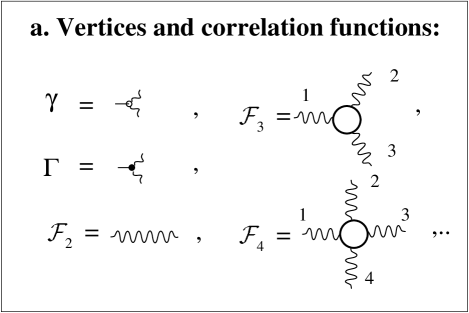
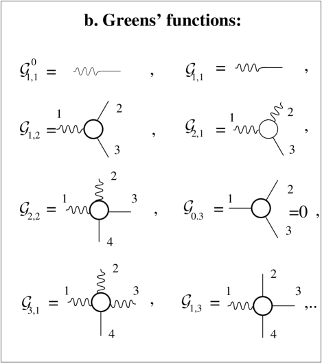
FIG. 1.: The diagrammatic notation of the basic objects of the theory. Panel a: the vertex $\gamma$ and the correlation functions ${\cal F}_{n}$ with $n=2,3,4$. Panel b: the bare Green’s function ${\cal G}^{0}_{1,1}$ (thin line), and the dressed Green’s functions ${\cal G}_{n,m}$. Objects with only straight tails are identically zero.

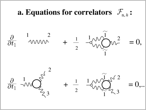
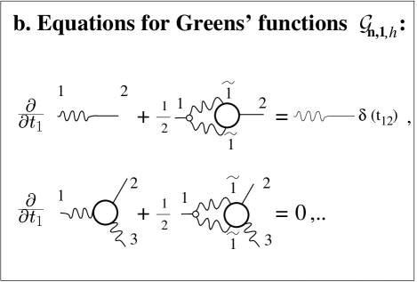
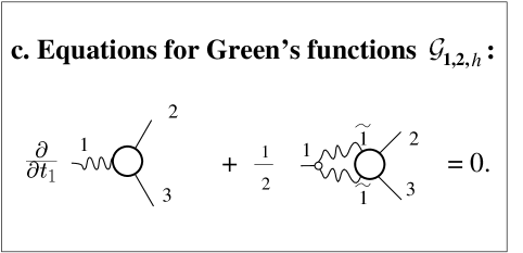
FIG. 2.: Diagrammatic reprezentation of the five equations for the lowest nontrivial ${\cal Z}$-covarian closure.

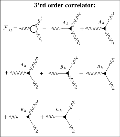
FIG. 3.: Exact reprezentation of the third-order correlation function

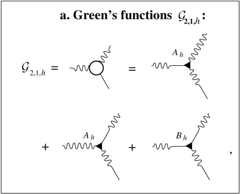
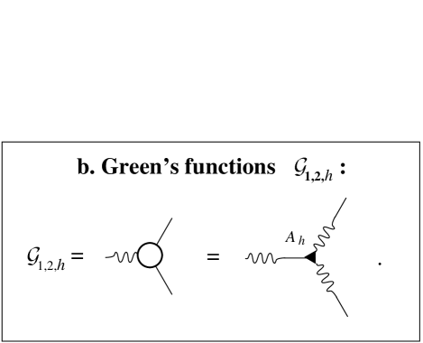
FIG. 4.: Exact representation of the nonlinear Green’s functions ${\cal G}_{2,1}$ and ${\cal G}_{1,2}.$

These five equations are presented symbolically in Fig. 2 and the symbols are explained in Fig. 1. We now show that in the first step of the closure procedure these five equations can be considered as ${\cal Z}(h)$-covariant equations for five unknowns. These five objects are the 2nd order correlation function ${\mathchoice{{\hbox{\boldmath$\displaystyle\cal F$}}}{{\hbox{\boldmath$\textstyle\cal F$}}}{{\hbox{\boldmath$\scriptstyle\cal F$}}}{{\hbox{\boldmath$\scriptscriptstyle\cal F$}}}}_{2,h}$, the regular Green’s function ${\mathchoice{{\hbox{\boldmath$\displaystyle\cal G$}}}{{\hbox{\boldmath$\textstyle\cal G$}}}{{\hbox{\boldmath$\scriptstyle\cal G$}}}{{\hbox{\boldmath$\scriptscriptstyle\cal G$}}}}_{1,1,h}$, and three types of triple vertices. The vertices are introduced in Figs. 3 and 4. We have in these figures three relationships that define the vertices ${\mathchoice{{\hbox{\boldmath$\displaystyle A$}}}{{\hbox{\boldmath$\textstyle A$}}}{{\hbox{\boldmath$\scriptstyle A$}}}{{\hbox{\boldmath$\scriptscriptstyle A$}}}}_{h}$, ${\mathchoice{{\hbox{\boldmath$\displaystyle B$}}}{{\hbox{\boldmath$\textstyle B$}}}{{\hbox{\boldmath$\scriptstyle B$}}}{{\hbox{\boldmath$\scriptscriptstyle B$}}}}_{h}$ and ${\mathchoice{{\hbox{\boldmath$\displaystyle C$}}}{{\hbox{\boldmath$\textstyle C$}}}{{\hbox{\boldmath$\scriptstyle C$}}}{{\hbox{\boldmath$\scriptscriptstyle C$}}}}_{h}$ on an “h-slice” in terms of ${\mathchoice{{\hbox{\boldmath$\displaystyle\cal F$}}}{{\hbox{\boldmath$\textstyle\cal F$}}}{{\hbox{\boldmath$\scriptstyle\cal F$}}}{{\hbox{\boldmath$\scriptscriptstyle\cal F$}}}}_{3,h}$, ${\mathchoice{{\hbox{\boldmath$\displaystyle\cal G$}}}{{\hbox{\boldmath$\textstyle\cal G$}}}{{\hbox{\boldmath$\scriptstyle\cal G$}}}{{\hbox{\boldmath$\scriptscriptstyle\cal G$}}}}_{2,1,h}$ and ${\mathchoice{{\hbox{\boldmath$\displaystyle\cal G$}}}{{\hbox{\boldmath$\textstyle\cal G$}}}{{\hbox{\boldmath$\scriptstyle\cal G$}}}{{\hbox{\boldmath$\scriptscriptstyle\cal G$}}}}_{1,2,h}$. Note that there is no notion of perturbation theory here - we simply define the three vertices in terms of objects that appear in Eqs. (52),(60) and (56).

Eq. (54) involves the 4th point correlator ${\mathchoice{{\hbox{\boldmath$\displaystyle\cal F$}}}{{\hbox{\boldmath$\textstyle\cal F$}}}{{\hbox{\boldmath$\scriptstyle\cal F$}}}{{\hbox{\boldmath$\scriptscriptstyle\cal F$}}}}_{4,h}$, Eq. (58) and Eq. (60) involve ${\mathchoice{{\hbox{\boldmath$\displaystyle\cal G$}}}{{\hbox{\boldmath$\textstyle\cal G$}}}{{\hbox{\boldmath$\scriptstyle\cal G$}}}{{\hbox{\boldmath$\scriptscriptstyle\cal G$}}}}_{3,1,h}$ and ${\mathchoice{{\hbox{\boldmath$\displaystyle\cal G$}}}{{\hbox{\boldmath$\textstyle\cal G$}}}{{\hbox{\boldmath$\scriptstyle\cal G$}}}{{\hbox{\boldmath$\scriptscriptstyle\cal G$}}}}_{2,2,h}$. These are 4th order objects, and we present them in Figs. 5 terms of all the possible decompositions made of lower order objects, and in addition new (“irreducible”) contributions which are defined by these relations. In order to have a consistent definition we need to add to this game the Green’s function ${\mathchoice{{\hbox{\boldmath$\displaystyle\cal G$}}}{{\hbox{\boldmath$\textstyle\cal G$}}}{{\hbox{\boldmath$\scriptstyle\cal G$}}}{{\hbox{\boldmath$\scriptscriptstyle\cal G$}}}}_{1,3,h}$. In the context of the 4th order objects the irreducible contributions are denoted symbolically as empty squares. There are four of them, and we denote them as ${\mathchoice{{\hbox{\boldmath$\displaystyle D$}}}{{\hbox{\boldmath$\textstyle D$}}}{{\hbox{\boldmath$\scriptstyle D$}}}{{\hbox{\boldmath$\scriptscriptstyle D$}}}}_{3,1,h}$, ${\mathchoice{{\hbox{\boldmath$\displaystyle D$}}}{{\hbox{\boldmath$\textstyle D$}}}{{\hbox{\boldmath$\scriptstyle D$}}}{{\hbox{\boldmath$\scriptscriptstyle D$}}}}_{2,2,h}$, ${\mathchoice{{\hbox{\boldmath$\displaystyle D$}}}{{\hbox{\boldmath$\textstyle D$}}}{{\hbox{\boldmath$\scriptstyle D$}}}{{\hbox{\boldmath$\scriptscriptstyle D$}}}}_{1,3,h}$ and ${\mathchoice{{\hbox{\boldmath$\displaystyle D$}}}{{\hbox{\boldmath$\textstyle D$}}}{{\hbox{\boldmath$\scriptstyle D$}}}{{\hbox{\boldmath$\scriptscriptstyle D$}}}}_{0,4,h}$. The first index stands for the number of wavy “tails” and the second index for the number of straight tails of the empty square.

A Systematic Closure

The first step of closure consists of discarding the irreducible empty squares. After doing so, we remain with precisely five equations (52)– (60) for five unknown functions. In the next step of closure we retain the empty squares as defined by their relations to the 4th order correlation and Green’s function, and add to the list of equations on an “h-slice” the equations of motion for the 4th order objects, i.e. ${\mathchoice{{\hbox{\boldmath$\displaystyle\cal F$}}}{{\hbox{\boldmath$\textstyle\cal F$}}}{{\hbox{\boldmath$\scriptstyle\cal F$}}}{{\hbox{\boldmath$\scriptscriptstyle\cal F$}}}}_{4,h}$, ${\mathchoice{{\hbox{\boldmath$\displaystyle\cal G$}}}{{\hbox{\boldmath$\textstyle\cal G$}}}{{\hbox{\boldmath$\scriptstyle\cal G$}}}{{\hbox{\boldmath$\scriptscriptstyle\cal G$}}}}_{3,1,h}$, ${\mathchoice{{\hbox{\boldmath$\displaystyle\cal G$}}}{{\hbox{\boldmath$\textstyle\cal G$}}}{{\hbox{\boldmath$\scriptstyle\cal G$}}}{{\hbox{\boldmath$\scriptscriptstyle\cal G$}}}}_{2,2,h}$ and ${\mathchoice{{\hbox{\boldmath$\displaystyle\cal G$}}}{{\hbox{\boldmath$\textstyle\cal G$}}}{{\hbox{\boldmath$\scriptstyle\cal G$}}}{{\hbox{\boldmath$\scriptscriptstyle\cal G$}}}}_{1,3,h}$. In total we have at this point nine equations. These equations will involve four 5th order objects, i.e. ${\mathchoice{{\hbox{\boldmath$\displaystyle\cal F$}}}{{\hbox{\boldmath$\textstyle\cal F$}}}{{\hbox{\boldmath$\scriptstyle\cal F$}}}{{\hbox{\boldmath$\scriptscriptstyle\cal F$}}}}_{5,h}$, ${\mathchoice{{\hbox{\boldmath$\displaystyle\cal G$}}}{{\hbox{\boldmath$\textstyle\cal G$}}}{{\hbox{\boldmath$\scriptstyle\cal G$}}}{{\hbox{\boldmath$\scriptscriptstyle\cal G$}}}}_{4,1,h}$, ${\mathchoice{{\hbox{\boldmath$\displaystyle\cal G$}}}{{\hbox{\boldmath$\textstyle\cal G$}}}{{\hbox{\boldmath$\scriptstyle\cal G$}}}{{\hbox{\boldmath$\scriptscriptstyle\cal G$}}}}_{3,2,h}$ and ${\mathchoice{{\hbox{\boldmath$\displaystyle\cal G$}}}{{\hbox{\boldmath$\textstyle\cal G$}}}{{\hbox{\boldmath$\scriptstyle\cal G$}}}{{\hbox{\boldmath$\scriptscriptstyle\cal G$}}}}_{2,3,h}$. Each of these new objects can be written now in terms of all the contributions that can be made from low order objects, plus irreducible 5th order vertices that we denote as empty pentagons. The second step of closure consists of discarding the empty pentagons. This gives us precisely nine equations for nine unknown functions, i.e. ${\mathchoice{{\hbox{\boldmath$\displaystyle\cal F$}}}{{\hbox{\boldmath$\textstyle\cal F$}}}{{\hbox{\boldmath$\scriptstyle\cal F$}}}{{\hbox{\boldmath$\scriptscriptstyle\cal F$}}}}_{2,h}$, ${\mathchoice{{\hbox{\boldmath$\displaystyle\cal G$}}}{{\hbox{\boldmath$\textstyle\cal G$}}}{{\hbox{\boldmath$\scriptstyle\cal G$}}}{{\hbox{\boldmath$\scriptscriptstyle\cal G$}}}}_{1,1,h}$, ${\mathchoice{{\hbox{\boldmath$\displaystyle A$}}}{{\hbox{\boldmath$\textstyle A$}}}{{\hbox{\boldmath$\scriptstyle A$}}}{{\hbox{\boldmath$\scriptscriptstyle A$}}}}_{h}$, ${\mathchoice{{\hbox{\boldmath$\displaystyle B$}}}{{\hbox{\boldmath$\textstyle B$}}}{{\hbox{\boldmath$\scriptstyle B$}}}{{\hbox{\boldmath$\scriptscriptstyle B$}}}}_{h}$, ${\mathchoice{{\hbox{\boldmath$\displaystyle C$}}}{{\hbox{\boldmath$\textstyle C$}}}{{\hbox{\boldmath$\scriptstyle C$}}}{{\hbox{\boldmath$\scriptscriptstyle C$}}}}_{h}$, and the four empty square vertices ${\mathchoice{{\hbox{\boldmath$\displaystyle D$}}}{{\hbox{\boldmath$\textstyle D$}}}{{\hbox{\boldmath$\scriptstyle D$}}}{{\hbox{\boldmath$\scriptscriptstyle D$}}}}_{3,1,h}$, ${\mathchoice{{\hbox{\boldmath$\displaystyle D$}}}{{\hbox{\boldmath$\textstyle D$}}}{{\hbox{\boldmath$\scriptstyle D$}}}{{\hbox{\boldmath$\scriptscriptstyle D$}}}}_{2,2,h}$, ${\mathchoice{{\hbox{\boldmath$\displaystyle D$}}}{{\hbox{\boldmath$\textstyle D$}}}{{\hbox{\boldmath$\scriptstyle D$}}}{{\hbox{\boldmath$\scriptscriptstyle D$}}}}_{1,3,h}$ and ${\mathchoice{{\hbox{\boldmath$\displaystyle D$}}}{{\hbox{\boldmath$\textstyle D$}}}{{\hbox{\boldmath$\scriptstyle D$}}}{{\hbox{\boldmath$\scriptscriptstyle D$}}}}_{0,4,h}$.

The procedure is now clear in its entirety. At the $n$th step of the closure we will discard the $n+3$th irreducible contributions, and will have precisely the right number of equations on an “$h$-slice” to solve for the remaining unknowns. We should stress that this procedure is not perturbative since we solve the exact equations on an “$h$-slice”. Our presentation of $n$th order objects on the “$h$-slice” in terms of lower order ones is also exact, it just defines at the $n$th step of the procedure a group of $(n+3)$th new vertices. These vertices are solved for only at the $(n+1)$th step of the procedure, when the $(n+4)$th vertices are discarded.

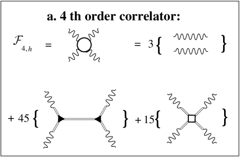
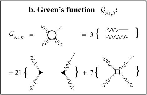
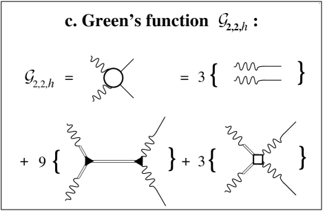
FIG. 5.: Exact representation of the forth-oredr correlation function (Panel a) and nonlinear Green’s functions (Panels b and c). Empty squares reprezent irreducible contributions to the 4th order vertices which are neglected in the lowest order ${\cal Z}$-covariant closure. Double line represent either wavy or straight line. For more details see Paper I.

It would be only fair to say that the idea for this procedure came from a careful examination of the fully renormalized perturbation theory for this problem, [1]. In that procedure one can derive equations for the $nth$ order objects that appear symbolically like Figs. 5a, 5b. etc. In addition, one can at each step of the procedure have an infinite expansion for the irreducible contributions. Nevertheless, the procedure explained above is different; firstly, it is consistently developed on an “$h$-slice”, whereas the renormalized perturbation theory is done for the standard statistical objects. Secondly, at no point is there any infinite expansion whose convergence properties are dubious. We just go through a set of explicit definitions solving an exact set of equations. The only question that needs to be understood is the speed of convergence of this scheme in terms of the scalar function ${\cal Z}(h)$ which parametrizes the anomalous behavior.

B ${\cal Z}$-covariance

A crucial property of our closure procedure is that it guarantees that power counting remains irrelevant on an “$h$-slice” for an arbitrary step of the procedure, and the scalar function ${\cal Z}(h)$ cannot be computed from power counting. To see this we need to find the rescaling properties of the triple and higher order vertices. We start with the triple vertices ${\mathchoice{{\hbox{\boldmath$\displaystyle A$}}}{{\hbox{\boldmath$\textstyle A$}}}{{\hbox{\boldmath$\scriptstyle A$}}}{{\hbox{\boldmath$\scriptscriptstyle A$}}}}_{h}$, ${\mathchoice{{\hbox{\boldmath$\displaystyle B$}}}{{\hbox{\boldmath$\textstyle B$}}}{{\hbox{\boldmath$\scriptstyle B$}}}{{\hbox{\boldmath$\scriptscriptstyle B$}}}}_{h}$ and ${\mathchoice{{\hbox{\boldmath$\displaystyle C$}}}{{\hbox{\boldmath$\textstyle C$}}}{{\hbox{\boldmath$\scriptstyle C$}}}{{\hbox{\boldmath$\scriptscriptstyle C$}}}}_{h}$. The first one is defined by its relation to ${\mathchoice{{\hbox{\boldmath$\displaystyle\cal G$}}}{{\hbox{\boldmath$\textstyle\cal G$}}}{{\hbox{\boldmath$\scriptstyle\cal G$}}}{{\hbox{\boldmath$\scriptscriptstyle\cal G$}}}}_{1,2,h}$, see Fig. 4b. Using the facts that

$${\mathchoice{{\hbox{\boldmath$\displaystyle\cal F$}}}{{\hbox{\boldmath$\textstyle\cal F$}}}{{\hbox{\boldmath$\scriptstyle\cal F$}}}{{\hbox{\boldmath$\scriptscriptstyle\cal F$}}}}_{2,h} \to \lambda^{2h+{\cal Z}(h)}{\mathchoice{{\hbox{\boldmath$\displaystyle\cal F$}}}{{\hbox{\boldmath$\textstyle\cal F$}}}{{\hbox{\boldmath$\scriptstyle\cal F$}}}{{\hbox{\boldmath$\scriptscriptstyle\cal F$}}}}_{2,h}\ ,$$ (62)

$${\mathchoice{{\hbox{\boldmath$\displaystyle\cal G$}}}{{\hbox{\boldmath$\textstyle\cal G$}}}{{\hbox{\boldmath$\scriptstyle\cal G$}}}{{\hbox{\boldmath$\scriptscriptstyle\cal G$}}}}_{1,1,h} \to \lambda^{{\cal Z}(h)-3}{\mathchoice{{\hbox{\boldmath$\displaystyle\cal G$}}}{{\hbox{\boldmath$\textstyle\cal G$}}}{{\hbox{\boldmath$\scriptstyle\cal G$}}}{{\hbox{\boldmath$\scriptscriptstyle\cal G$}}}}_{1,1,h}\ ,$$ (63)

$${\mathchoice{{\hbox{\boldmath$\displaystyle\cal G$}}}{{\hbox{\boldmath$\textstyle\cal G$}}}{{\hbox{\boldmath$\scriptstyle\cal G$}}}{{\hbox{\boldmath$\scriptscriptstyle\cal G$}}}}_{1,2,h} \to \lambda^{-h+{\cal Z}(h)-6}{\mathchoice{{\hbox{\boldmath$\displaystyle\cal G$}}}{{\hbox{\boldmath$\textstyle\cal G$}}}{{\hbox{\boldmath$\scriptstyle\cal G$}}}{{\hbox{\boldmath$\scriptscriptstyle\cal G$}}}}_{1,2,h}\ ,.$$ (64)

we find that ${\mathchoice{{\hbox{\boldmath$\displaystyle A$}}}{{\hbox{\boldmath$\textstyle A$}}}{{\hbox{\boldmath$\scriptstyle A$}}}{{\hbox{\boldmath$\scriptscriptstyle A$}}}}_{h}$ has to transform according to

$${\mathchoice{{\hbox{\boldmath$\displaystyle A$}}}{{\hbox{\boldmath$\textstyle A$}}}{{\hbox{\boldmath$\scriptstyle A$}}}{{\hbox{\boldmath$\scriptscriptstyle A$}}}}_{h}\to\lambda^{2h-2{\cal Z}(h)-9}{\mathchoice{{\hbox{\boldmath$\displaystyle A$}}}{{\hbox{\boldmath$\textstyle A$}}}{{\hbox{\boldmath$\scriptstyle A$}}}{{\hbox{\boldmath$\scriptscriptstyle A$}}}}_{h}\ .$$ (65)

Armed with this knowledge we proceed to the definition of ${\mathchoice{{\hbox{\boldmath$\displaystyle B$}}}{{\hbox{\boldmath$\textstyle B$}}}{{\hbox{\boldmath$\scriptstyle B$}}}{{\hbox{\boldmath$\scriptscriptstyle B$}}}}_{h}$ through its relation to ${\mathchoice{{\hbox{\boldmath$\displaystyle\cal G$}}}{{\hbox{\boldmath$\textstyle\cal G$}}}{{\hbox{\boldmath$\scriptstyle\cal G$}}}{{\hbox{\boldmath$\scriptscriptstyle\cal G$}}}}_{2,1,h}$, equation in Fig. 4a. We can check that the rescaling property of

$${\mathchoice{{\hbox{\boldmath$\displaystyle\cal G$}}}{{\hbox{\boldmath$\textstyle\cal G$}}}{{\hbox{\boldmath$\scriptstyle\cal G$}}}{{\hbox{\boldmath$\scriptscriptstyle\cal G$}}}}_{2,1,h}\to\lambda^{h+{\cal Z}(h)-3}{\mathchoice{{\hbox{\boldmath$\displaystyle\cal G$}}}{{\hbox{\boldmath$\textstyle\cal G$}}}{{\hbox{\boldmath$\scriptstyle\cal G$}}}{{\hbox{\boldmath$\scriptscriptstyle\cal G$}}}}_{1,2,h}$$ (66)

agrees exactly with the two terms that contain the vertex ${\mathchoice{{\hbox{\boldmath$\displaystyle A$}}}{{\hbox{\boldmath$\textstyle A$}}}{{\hbox{\boldmath$\scriptstyle A$}}}{{\hbox{\boldmath$\scriptscriptstyle A$}}}}_{h}$ on the RHS. Accordingly also the term containing ${\mathchoice{{\hbox{\boldmath$\displaystyle B$}}}{{\hbox{\boldmath$\textstyle B$}}}{{\hbox{\boldmath$\scriptstyle B$}}}{{\hbox{\boldmath$\scriptscriptstyle B$}}}}_{h}$ has to transform in the same way, leading to

$${\mathchoice{{\hbox{\boldmath$\displaystyle B$}}}{{\hbox{\boldmath$\textstyle B$}}}{{\hbox{\boldmath$\scriptstyle B$}}}{{\hbox{\boldmath$\scriptscriptstyle B$}}}}_{h}\to\lambda^{4h-2{\cal Z}(h)-6}{\mathchoice{{\hbox{\boldmath$\displaystyle B$}}}{{\hbox{\boldmath$\textstyle B$}}}{{\hbox{\boldmath$\scriptstyle B$}}}{{\hbox{\boldmath$\scriptscriptstyle B$}}}}_{h}\ .$$ (67)

In making this assertion we assumed that there is no cancellation of the leading terms in the equation. Otherwise the vertex ${\mathchoice{{\hbox{\boldmath$\displaystyle B$}}}{{\hbox{\boldmath$\textstyle B$}}}{{\hbox{\boldmath$\scriptstyle B$}}}{{\hbox{\boldmath$\scriptscriptstyle B$}}}}_{h}$ would be smaller. Lastly we use the definition of ${\mathchoice{{\hbox{\boldmath$\displaystyle C$}}}{{\hbox{\boldmath$\textstyle C$}}}{{\hbox{\boldmath$\scriptstyle C$}}}{{\hbox{\boldmath$\scriptscriptstyle C$}}}}_{h}$ by the relation to ${\mathchoice{{\hbox{\boldmath$\displaystyle\cal F$}}}{{\hbox{\boldmath$\textstyle\cal F$}}}{{\hbox{\boldmath$\scriptstyle\cal F$}}}{{\hbox{\boldmath$\scriptscriptstyle\cal F$}}}}_{3,h}$, see Fig. 3, that transforms like

$${\mathchoice{{\hbox{\boldmath$\displaystyle\cal F$}}}{{\hbox{\boldmath$\textstyle\cal F$}}}{{\hbox{\boldmath$\scriptstyle\cal F$}}}{{\hbox{\boldmath$\scriptscriptstyle\cal F$}}}}_{3,h}\to\lambda^{3h+{\cal Z}(h)}{\mathchoice{{\hbox{\boldmath$\displaystyle\cal F$}}}{{\hbox{\boldmath$\textstyle\cal F$}}}{{\hbox{\boldmath$\scriptstyle\cal F$}}}{{\hbox{\boldmath$\scriptscriptstyle\cal F$}}}}_{3,h}\ .$$ (68)

All the terms that include ${\mathchoice{{\hbox{\boldmath$\displaystyle A$}}}{{\hbox{\boldmath$\textstyle A$}}}{{\hbox{\boldmath$\scriptstyle A$}}}{{\hbox{\boldmath$\scriptscriptstyle A$}}}}_{h}$ and ${\mathchoice{{\hbox{\boldmath$\displaystyle B$}}}{{\hbox{\boldmath$\textstyle B$}}}{{\hbox{\boldmath$\scriptstyle B$}}}{{\hbox{\boldmath$\scriptscriptstyle B$}}}}_{h}$ have the same rescaling exponent as that of ${\mathchoice{{\hbox{\boldmath$\displaystyle\cal F$}}}{{\hbox{\boldmath$\textstyle\cal F$}}}{{\hbox{\boldmath$\scriptstyle\cal F$}}}{{\hbox{\boldmath$\scriptscriptstyle\cal F$}}}}_{3,h}$. We can therefore find the rescaling exponent of ${\mathchoice{{\hbox{\boldmath$\displaystyle C$}}}{{\hbox{\boldmath$\textstyle C$}}}{{\hbox{\boldmath$\scriptstyle C$}}}{{\hbox{\boldmath$\scriptscriptstyle C$}}}}_{h}$:

$${\mathchoice{{\hbox{\boldmath$\displaystyle C$}}}{{\hbox{\boldmath$\textstyle C$}}}{{\hbox{\boldmath$\scriptstyle C$}}}{{\hbox{\boldmath$\scriptscriptstyle C$}}}}_{h}\to\lambda^{6h-2{\cal Z}(h)-3}{\mathchoice{{\hbox{\boldmath$\displaystyle C$}}}{{\hbox{\boldmath$\textstyle C$}}}{{\hbox{\boldmath$\scriptstyle C$}}}{{\hbox{\boldmath$\scriptscriptstyle C$}}}}_{h}\ .$$ (69)

We again assumed that there is no cancellation of the leading terms in the equation for ${\mathchoice{{\hbox{\boldmath$\displaystyle\cal F$}}}{{\hbox{\boldmath$\textstyle\cal F$}}}{{\hbox{\boldmath$\scriptstyle\cal F$}}}{{\hbox{\boldmath$\scriptscriptstyle\cal F$}}}}_{3,h}$. If there is cancellation, the vertex ${\mathchoice{{\hbox{\boldmath$\displaystyle C$}}}{{\hbox{\boldmath$\textstyle C$}}}{{\hbox{\boldmath$\scriptstyle C$}}}{{\hbox{\boldmath$\scriptscriptstyle C$}}}}_{h}$ can be smaller.

At this point we can check that the first step in our closure scheme leads to a ${\cal Z}(h)$ covariant procedure. Consider firstly the three contributions of Gaussian decomposition which are first on the RHS of the equation in Fig. 5a. These rescale like $\lambda^{4h+2{\cal Z}(h)}$, and their ratio to the LHS is proportional to $(R/L)^{{\cal Z}(h)}$. For ${\cal Z}(h)$ positive these contributions become irrelevant in the limit $(R/L)\to 0$. The 45 contributions that come next contain pairs of triple vertices, and we need to use the rescaling properties (65), (67), and (69) to find their rescaling exponents. We find that they all share the same rescaling exponent . In hindsight this should not be surprising. This is a result of the assumption that in the definitions of the three vertices there are no cancellations in the leading scaling behavior. Thus the rescaling exponent of all the 45 contributions could be obtained from analyzing one of them. The nontrivial fact is that the common rescaling of all these terms is exactly the rescaling of the LHS of the equation, which is $\lambda^{4h+{\cal Z}(h)}$ . This means that our closure for the 4th order correlation functions cannot introduce power counting. Note that the rescaling neutrality with respect to counting of $h$ and of natural numbers follows from the rescaling symmetry of the Euler equation, and is shared also by Gaussian contributions. On the other hand the neutrality with respect to ${\cal Z}(h)$ is nontrivial, and follows from a judicious choice of the proposed closure scheme. We will refer this property as ${\cal Z}$-covariance.

It is important to understand now that the proposed closures for the other 4th order objects, like Fig. 5b are also ${\cal Z}$-covariant. All that changes is the number of wavy and straight tails on the LHS and RHS of the equations, and the rescaling exponents change in the same way on the two sides of the equation.

We can now consider the next step of closure, taking into account the irreducible 4th order vertices (empty squares), discarding the 5th order empty pentagons (irreducible contributions, for details, see Paper 1 The procedure follows verbatim the one described above for the triple vertices and the rescaling exponents of the irreducible 4th order vertices ${\mathchoice{{\hbox{\boldmath$\displaystyle D$}}}{{\hbox{\boldmath$\textstyle D$}}}{{\hbox{\boldmath$\scriptstyle D$}}}{{\hbox{\boldmath$\scriptscriptstyle D$}}}}_{m,n,h}$ are determined:

$${\mathchoice{{\hbox{\boldmath$\displaystyle D$}}}{{\hbox{\boldmath$\textstyle D$}}}{{\hbox{\boldmath$\scriptstyle D$}}}{{\hbox{\boldmath$\scriptscriptstyle D$}}}}_{m,n,h} \to \lambda^{d_{m,n}(h)}{\mathchoice{{\hbox{\boldmath$\displaystyle D$}}}{{\hbox{\boldmath$\textstyle D$}}}{{\hbox{\boldmath$\scriptstyle D$}}}{{\hbox{\boldmath$\scriptscriptstyle D$}}}}_{m,n,h}\ ,$$ (70)

$$d_{m,n}(h) = 2nh-3{\cal Z}(h)-3m-4\ .$$ (71)

We can check the terms that appear in the 5th order correlation and Green’s functions, which are made of combinations of triple and 4th order vertices. We discover that all these terms share the same rescaling exponent, and that it agrees precisely with the rescaling of the 5th order correlation and Green’s function. Accordingly also the second step of closure is ${\cal Z}$-covariant.

It becomes evident that we develop a systematic ${\cal Z}$-covariant closure scheme, and that power counting will not creep in at any step of the procedure. In the next section we show that the scalar function ${\cal Z}(h)$ can be computed from this scheme as a generalized eigenvalue. We also explain the role of the boundary conditions in the space of scales, and how the re-normalization scale is chosen.

4 The scalar function ${\cal Z}$ as a generalized eigenvalue

In this section we demonstrate that at any step of our closure, the scalar function ${\cal Z}(h)$ can be found only from a solvability condition. We will also explain the role of the boundary conditions in the space of scales in determining the scaling functions in this theory.

The point is really rather simple. First observe that our initial equations for correlation and Green’s functions on an “$h$-slice”, like (34) or (56)-(60) are linear functional equations. The equations for the correlation functions are not only linear, but also homogeneous. The equations for the Green’s functions are not all homogeneous, but as we explained in the last section the inhomogeneous terms are much smaller than the homogeneous terms in the limit $(R/L)\to 0$, and they can be discarded. This means, of course, that all the functions on an “$h$-slice” can be determined only up to an over all numerical constant. At this point we may have even more than one overall free constant; on the face of it the equations for the correlation functions are independent of the equations for the Green’s functions, and we can have different overall constants in the correlation and the Green’s functions.

Every step of closure turns a set of linear functional equations into a set of nonlinear functional equations. We claim that nevertheless all the functions appearing in these equations can be determined only up to an overall numerical constant. The extra freedom of many possible constants disappears now, since the correlation and the Green’s functions are coupled after closure. But one overall constant remains free. The reason is of course the property of ${\cal Z}$-covariance, which includes as a special case invariance to an overall scaling factor, or rescaling by $\lambda^{0}$.

If our equations were linear, this freedom would have meant that we need to require the standard solvability condition that the linear operator had an eigenvalue zero, and the functions that we seek would have been identified as the “zero-modes” associated with this eigenvalue. Our equations are not linear, and the solvability condition is not that simple. Nevertheless we know apriori that at every step of the closure we will need to find the solvability condition of the nonlinear set of equations, and this condition will determine the numerical value of ${\cal Z}(h)$.

Even after determining ${\cal Z}(h)$ the statistical functions will be determined only up to a factor which may depend on $h$, which is the measure $\mu(h)$ in Eqs(24) and (49). In order to determine this factor we will need to fit all correlation functions ${\mathchoice{{\hbox{\boldmath$\displaystyle T$}}}{{\hbox{\boldmath$\textstyle T$}}}{{\hbox{\boldmath$\scriptstyle T$}}}{{\hbox{\boldmath$\scriptscriptstyle T$}}}}_{n}$ to the boundary conditions in the space of scales. At that point the computed values of ${\cal Z}(h)$ will determine whether it is the inner or the outer scale of turbulence that appears as the renormalizaiton scale. We will show in the lowest step of closure that the outer scale $L$ is selected.

5 Summary and the Road Ahead

Up to now we described the general ideas and how the closure scheme should work. The main point of the analysis is that the equations of motion of the statistical objects admit an exact rescaling group that contains, for a given “$h$-slice”, one unknown scalar function ${\cal Z}(h)$ whose calculation is sufficient for the evaluation of the scaling exponents $\zeta_{n}$ via Eq. (18).

Unfortunately, the actual calculations that are called for in this scheme are far from trivial. In the lowest step of closure we are faced with five coupled integro-differential equations in many space-time variables, and the complexity increases rapidly in the higher steps of closure. We are currently attempting to solve numerically the lowest step of closure with the aim of demonstrating the existence of anomalous scaling. We are not particularly interested in the first step in precise values of the exponents $\zeta_{n}$, it is more important to show that they differ from their K41 counterparts. Numerical accuracy and the convergence of ${\cal Z}(h)$ will be examined in the higher steps of closure. The complexity of the numerics means that this is a long program that is expected to last for a couple of years. For this reason we chose to describe the ideas of the closure scheme even at this stage when the numerical implementation is lacking. It is our feeling that the procedure is sound and that there is a good chance to obtain results that will justify the effort that is called for in the numerical implementation.