PHYSICAL REVIEW E Version of
  
Computing the Scaling Exponents in Fluid Turbulence from First Principles:
the Formal Setup

Abstract

We propose a scheme for the calculation from the Navier-Stokes equations of the scaling exponents $\zeta_{n}$ of the $n$th order correlation functions in fully developed hydrodynamic turbulence. The scheme is nonperturbative and constructed to respect the fundamental rescaling symmetry of the Euler equation. It constitutes an infinite hierarchy of coupled equations that are obeyed identically with respect to scaling for any set of scaling exponents $\zeta_{n}$. As a consequence the scaling exponents are determined by solvability conditions and not from power counting. It is argued that in order to achieve such a formulation one must recognize that the many-point space-time correlation functions are not scale invariant in their time arguments. The assumption of full scale invariance leads unavoidably to Kolmogorov exponents. It is argued that the determination of of all the scaling exponents $\zeta_{n}$ requires equations for infinitely many renormalized objects. One can however proceed in controlled successive approximations by successive truncations of the infinite hierarchy of equations.Clues as to how to truncate without reintroducing power counting can be obtained from renormalized perturbation theory. To this aim we show that the fully resummed perturbation theory is equivalent in its contents to the exact hierarchy of equations obeyed by the $n$th order correlation functions and Green’s function. In light of this important result we can safely use finite resummations to construct successive closures of the infinite hierarchy of equations. This paper presents the conceptual and technical details of the scheme. The analysis of the high-order closure procedures which do not destroy the rescaling symmetry and the actual calculations fWork4or truncated models will be presented in a forthcoming paper in collaboration with V. Belinicher.

1 Introduction

The aim of this paper is to present a general scheme for the calculation of the scaling exponents characterizing the statistical quantities that arise in the description of fully developed hydrodynamic turbulence. These statistical quantities are various averages computed from the fundamental field in hydrodynamics, the velocity field of the fluid. Denote the Eulerian velocity field as ${{\bf{u}}}({{\bf{r}}},t)$ where ${\bf{r}}$ is a point in $d$-dimensional space (usually $d=2$ or 3) and $t$ is the time. Statistical quantities that have attracted years of experimental and theoretical attention [1, 2, 3, 4] are the structure functions of velocity differences, denoted as $S_{n}(R)$

$$S_{n}(R)=\left\langle|\hbox{{\bf{u}}}({{\bf{r}}}+{{\bf{R}}},t)-{{\bf{u}}}({{\bf{r}}},t)|^{n}\right\rangle\ ,$$ (1)

where $\left<\dots\right>$ stands for a suitably defined ensemble average. It has been asserted for a long time that the structure functions scale as a function of the separation $R$ according to

$$S_{n}(R)\sim R^{\zeta_{n}}\ ,$$ (2)

where $\zeta_{n}$ are known as the scaling exponents of the structure functions. It is assumed here that the separation $R$ lies in the so-called “inertial range”, i.e. $\eta\ll R\ll L$ with $\eta$ the inner viscous scale and $L$ the outer integral scale of turbulence. One of the major questions in fundamental turbulence research is whether these scaling exponents are correctly predicted by the classical Kolmogorov 41 theory in which $\zeta_{n}=n/3$, or if these exponents manifest the phenomenon of “multiscaling” with $\zeta_{n}$ a nonlinear function of $n$, as has been indicated by physical and numerical experiments [5, 6, 7, 8, 9].

In an attempt to develop a consistent theory of turbulence one may define statistical quantities that depend on many spatial and temporal coordinates. Defining the velocity difference ${{\bf{w}}}({{\bf{r}}},{{\bf{r}}}^{\prime},t)$ as

$${{\bf{w}}}({{\bf{r}}},{{\bf{r}}}^{\prime},t)\equiv{{\bf{u}}}({{\bf{r}}}^{\prime},t)-{{\bf{u}}}({{\bf{r}}},t)\ ,$$ (3)

one considers the $n$-rank tensor space-time correlation function

$${\bf{F}}_{n}({{\bf{r}}}_{1},{{\bf{r}}}^{\prime}_{1},t_{1};{{\bf{r}}}_{2},{{\bf{r}}}^{\prime}_{2},t_{2};\dots;{\bf{r}}_{n},{{\bf{r}}}^{\prime}_{n},t_{n})$$ (4)

$$= \left<{\bf{w}}({{\bf{r}}}_{1},{{\bf{r}}}^{\prime}_{1},t_{1}){\bf{w}}({{\bf{r}}}_{2},{{\bf{r}}}^{\prime}_{2},t_{2})\dots{\bf{w}}({{\bf{r}}}_{n},{{\bf{r}}}^{\prime}_{n},t_{n})\right>\ .$$ (5)

The simultaneous correlation function ${\bf{T}}_{n}$ is obtained from ${{\bf{F}}}_{n}$ when $t_{1}=t_{2}\dots=t_{n}$. In statistically stationary turbulence the equal time correlation function is time independent, and we denote it as

$${{\bf{T}}}_{n}({{\bf{r}}}_{1},{{\bf{r}}}^{\prime}_{1};{{\bf{r}}}_{2},{{\bf{r}}}^{\prime}_{2};\dots;{{\bf{r}}}_{n},{{\bf{r}}}^{\prime}_{n})$$ (6)

$$= \left<{\bf{w}}({{\bf{r}}}_{1},{{\bf{r}}}^{\prime}_{1},t){\bf{w}}({{\bf{r}}}_{2},{{\bf{r}}}^{\prime}_{2},t)\dots{\bf{w}}({{\bf{r}}}_{n},{{\bf{r}}}^{\prime}_{n},t)\right>\ .$$ (7)

One expects that when all the separations $R_{i}\equiv|{\bf{r}}_{i}-{\bf{r}}^{\prime}_{i}|$ are in the inertial range, $\eta\ll R_{i}\ll L$, the simultaneous correlation function is scale invariant in the sense that

$${{\bf{T}}}_{n}(\lambda{{\bf{r}}}_{1},\lambda{{\bf{r}}}^{\prime}_{1};\lambda{{\bf{r}}}_{2},\lambda{{\bf{r}}}^{\prime}_{2};\dots;\lambda{{\bf{r}}}_{n},\lambda{{\bf{r}}}^{\prime}_{n})$$ (8)

$$= \lambda^{\zeta_{n}}{{\bf{T}}}_{n}({{\bf{r}}}_{1},{{\bf{r}}}^{\prime}_{1};{{\bf{r}}}_{2},{{\bf{r}}}^{\prime}_{2};\dots;{{\bf{r}}}_{n},{{\bf{r}}}^{\prime}_{n})\ ,$$ (9)

and the exponent $\zeta_{n}$ is numerically the same as the one appearing in Eq. (2).

One of the major difference between the study of statistical turbulence and other examples of anomalous scaling in physics (like critical phenomena) is that there is no theory for the simultaneous correlation functions (7) that does not involve the many time correlation functions (5). Turbulence is a truly dynamical problem, and there is no free energy functional or a Boltzmann factor to provide a time-independent theory of the statistical weights. The theory for the simultaneous quantities (7) involves integrals over the time variables of the many time quantities (5). One must therefore learn how to perform these time integrations properly.

We propose here a point of departure from all previous attempts to compute the anomalous exponents $\zeta_{n}$ from first principles, based on the understanding that these functions are not scale invariant in their time arguments; this allows us to build a new approach. Naively one could assume that the scale invariance property extends to the time correlation functions in the sense that

$${{\bf{F}}}_{n}(\lambda{{\bf{r}}}_{1},\lambda{{\bf{r}}}^{\prime}_{1},\lambda^{z_{n}}t_{1};\dots;\lambda{{\bf{r}}}_{n},\lambda{{\bf{r}}}^{\prime}_{n},\lambda^{z_{n}}t_{n})$$ (10)

$$= \lambda^{\zeta_{n}}{{\bf{F}}}_{n}({{\bf{r}}}_{1},{{\bf{r}}}^{\prime}_{1},t_{1};\dots;{{\bf{r}}}_{n},{{\bf{r}}}^{\prime}_{n},t_{n})\ ,\quad({\rm not~{}true!})\ ,$$ (11)

with a dynamical scaling exponent $z_{n}$ which can be $n$ dependent. We have shown [10] that this is not the case, and in this paper we explain that using an adequate representation of the time dependence leads to a calculation scheme for the scaling exponents. We will reiterate that even in fully resummed theories, if we assume scale invariance in time we lose the availability of anomalous scaling in favor of K41 scaling. Full respect to the dynamical nature of the problem is required in order to proceed in understanding anomalous scaling.

Our strategy in developing a scheme of computation of the scaling exponents can be described as follows: The first step is to transform the Navier-Stokes equations using the Belinicher-L’vov transformation [11], see Eqs.(16)-(18). The resulting velocity field is denoted ${\bf{\cal W}}$, and the correlation function over these velocity fields is denoted ${\bf{\cal F}}_{n}$, see Eq. (26). Next we construct the infinite hierarchy of equations that relate the rate of change of the $n$th order correlation function ${\bf{\cal F}}_{n}$ to a space integral over a vertex convolved with the ($n+1$)th order correlation function ${\bf{\cal F}}_{n+1}$. This hierarchy is given by Eqs.(40),(48) below and it is exact. Next we explain, using the fusion rules [12, 13] that govern the asymptotic properties of the correlations functions when groups of their spatial arguments coalesce together, that the spatial integrals converge both in the UV and the IR limits. This result allows us to show that if Eq. (11) were true, the hierarchy of equations could be studied by power counting, and the only solution would be linear (i.e. $\zeta_{n}$ linear in $n$) rather than anomalous scaling. We will show that Eq. (11) is not true, and that the many-time correlation functions must be “multiscaling” in their time representation. This fact means that the hierarchy of equations cannot be studied by power counting. The next step is to represent the space and time dependent correlation functions in a way that exposes their multiscaling characteristics [10]. This form (83) is a convenient form that makes use of the “multifractal” representation, which was found useful before in the context of the simultaneous objects [4]. This representation amounts to saddle point integrals over correlation functions that respect the exact symmetry of the Euler equation, i.e. the symmetry of rescaling according to

$${\bf{r}}\to\lambda{\bf{r}},\quad{\bf{w}}\to\lambda^{h}{\bf{w}},\quad t\to\lambda^{1-h}t\ .$$ (12)

Using this representation we will see that the hierarchy of equations for the correlation functions is satisfied in the sense of power counting for any value of $h$, cf. Eq. (88). The information about the scaling exponents is hidden in the coefficients of the equation but cannot be read from power counting.

We are still faced with an infinite hierarchy of equations. This is not accidental; the calculation of infinitely many anomalous exponents in turbulence does indeed necessitate a calculation of infinitely many renormalized objects. Nevertheless we want to achieve a finite, approximate calculation of lower order exponents (i.e $\zeta_{n}$ with for the first integer values $n$). To this aim we need to truncate the infinite hierarchy of equations. The way to achieve an intelligent truncation can be seen from the study of renormalized perturbation theory [14]. Perturbative theories of turbulence have fallen into some ill-repute since the problem of turbulence does not have any small parameter that guarantees convergence of perturbative expansions. To increase our confidence in this approach, we first prove that the content of fully resummed perturbation theory is identical to the exact hierarchy of equations for $n$-order correlation functions and Green’s functions. This important result, which is demonstrated here for the first time, allows us to proceed safely in using partially resummed perturbation theory to guide our truncation of the hierarchy of exact equations. The clue is that we want to preserve the invariance of the theory under the rescaling (12). We outline how to do this in Section 8 and Appendix A of this paper. The actual analysis of the method of truncating while preserving the symmetry, and an approximate calculation of the low order exponents will be presented in a forthcoming paper [15]. Here we present the conceptual steps and technical issues.

2 Nonperturbative Formulation of the Statistical Theory of Turbulence

In order to derive anomalous exponents it is essential to develop a theory that is nonperturbative. In addition, one needs to deal with the effect of the sweeping of small scales by large scale motions. This effect is only kinematic, but it can mask the inherent time scales associated with nonlinear interactions, and therefore has to be carefully taken into account. To this aim we start this section with a short review of the equations of motion in the Belinicher-L’vov representation (subsection A), followed by the introduction of the statistical quantities of interest, which are $n$-order space time correlation functions and Green’s functions in subsection B. In subsection C we derive the exact hierarchy of equations satisfied by these quantities, the main results being Eqs. (40) (48) and (60).

A Equations of motion

The analytic theory of turbulence is based on the Navier-Stokes equation for the Eulerian velocity field ${{\bf{u}}}({{\bf{r}}},t)$. In the case of an incompressible fluid they read

$$\partial{{\bf{u}}}/\partial t+({{\bf{u}}}\cdot{\mathchoice{{\hbox{\boldmath$\displaystyle\nabla$}}}{{\hbox{\boldmath$\textstyle\nabla$}}}{{\hbox{\boldmath$\scriptstyle\nabla$}}}{{\hbox{\boldmath$\scriptscriptstyle\nabla$}}}}){{\bf{u}}}-\nu\nabla^{2}{{\bf{u}}}+{\mathchoice{{\hbox{\boldmath$\displaystyle\nabla$}}}{{\hbox{\boldmath$\textstyle\nabla$}}}{{\hbox{\boldmath$\scriptstyle\nabla$}}}{{\hbox{\boldmath$\scriptscriptstyle\nabla$}}}}p={{\bf{f}}},\quad{\mathchoice{{\hbox{\boldmath$\displaystyle\nabla$}}}{{\hbox{\boldmath$\textstyle\nabla$}}}{{\hbox{\boldmath$\scriptstyle\nabla$}}}{{\hbox{\boldmath$\scriptscriptstyle\nabla$}}}}\cdot{{\bf{u}}}=0\,,$$ (13)

where $\nu$ is the kinematic viscosity, $p$ is the pressure, and ${{\bf{f}}}$ is some forcing which maintains the flow. Since we are interested in incompressible flows, we project the longitudinal components out of the equations of motion. This is done with the help of the projection operator $\tensor{P}$ which is formally written as $\tensor{P}$ $\equiv-\nabla^{-2}{\mathchoice{{\hbox{\boldmath$\displaystyle\nabla$}}}{{\hbox{\boldmath$\textstyle\nabla$}}}{{\hbox{\boldmath$\scriptstyle\nabla$}}}{{\hbox{\boldmath$\scriptscriptstyle\nabla$}}}}\times{\mathchoice{{\hbox{\boldmath$\displaystyle\nabla$}}}{{\hbox{\boldmath$\textstyle\nabla$}}}{{\hbox{\boldmath$\scriptstyle\nabla$}}}{{\hbox{\boldmath$\scriptscriptstyle\nabla$}}}}\times$. Applying $\tensor{P}$ to Eq. (13) we find

$$(\partial/\partial t-\nu\nabla^{2}){{\bf{u}}}+\tensor{P}({{\bf{u}}}\cdot\mathchoice{{\hbox{\boldmath$\displaystyle\nabla$}}}{{\hbox{\boldmath$\textstyle\nabla$}}}{{\hbox{\boldmath$\scriptstyle\nabla$}}}{{\hbox{\boldmath$\scriptscriptstyle\nabla$}}}){{\bf{u}}}=\,\tensor{P}{{\bf{f}}}\ .$$ (14)

This equation has been used as a starting point for a field-theoretic perturbation theory, in which the nonlinear term acts as a “perturbation” on the linear part of the equation. Such an approach is fraught with difficulties simply because the natural statistical objects which appear in the perturbation expansions[16, 17, 18, 19] of the Navier-Stokes equation are correlation functions $\tilde{F}^{\alpha\beta}({\bf r},{{\bf{r}}}^{\prime},t,t^{\prime})$ of the velocity field ${{\bf{u}}}({{\bf{r}}},t)$ itself:

$$\tilde{F}^{\alpha\beta}({{\bf{r}}},{{\bf{r}}}^{\prime},t,t^{\prime})=\left\langle u^{\alpha}({{\bf{r}}},t)u^{\beta}({{\bf{r}}}^{\prime},t^{\prime})\right\rangle\ .$$ (15)

The problem is that the correlator $\tilde{F}^{\alpha\beta}({{\bf{r}}},{{\bf{r}}}^{\prime},t,t^{\prime})$ is not universal, since it is dominated by contributions to $u_{\alpha}({{\bf{r}}},t)$ which come from the largest scales in the fluid flow, and these are determined by the features of the energy injection mechanisms. This physical fact is reflected in the theory as infra-red divergences that have plagued the development of analytic approach for decades. Indeed, all the early attempts to develop a consistent analytic approach to turbulence, notably the well known theories of Wyld[16] and of Martin, Siggia and Rose[17], shared this problem. One needs to transform Eq. (13) such that the statistical objects that appear naturally will be written in terms of velocity differences which can be universal. We like to use the Belinicher-L’vov (BL) transformation for this purpose, but any other transformation that reaches the same goal is equally acceptable. We will stress that the results that we obtain below do not depend on the details of the transformation, and we employ the BL transformation because it is particularly straightforward. The equation of motion that is obtained from the BL-transformation is exact, and there is no approximation involved in this step. In terms of the Eulerian velocity ${{\bf{u}}}({{\bf{r}}},t)$ Belinicher and L’vov defined the field ${{\bf{v}}}({{\bf{r}}}_{0},t_{0}|{{\bf{r}}},t)$ as

$${{\bf{v}}}({{\bf{r}}}_{0},t_{0}|{{\bf{r}}},t)\equiv{{\bf{u}}}[{{\bf{r}}}+\mbox{\boldmath$\rho$}({{\bf{r}}}_{0},t),t]$$ (16)

where

$$\mbox{\boldmath$\rho$}({{\bf{r}}}_{0},t)=\int_{t_{0}}^{t}ds{{\bf{u}}}[{{\bf{r}}}_{0}+\mbox{\boldmath$\rho$}({{\bf{r}}}_{0},s),s]\ .$$ (17)

Note that $\mbox{\boldmath$\rho$}({{\bf{r}}}_{0},t)$ is precisely the Lagrangian trajectory of a fluid particle that is positioned at ${\bf r}_{0}$ at time $t=t_{0}$. The field ${{\bf{v}}}({\bf r}_{0},t_{0}|{{\bf{r}}},t)$ is simply the Eulerian field in the frame of reference of a single chosen material point ${\bf{\rho}}({\bf{r}}_{0},t)$. The observation of Belinicher and L’vov [11] was that the variables ${\bf{\cal W}}({\bf{r}}_{0},t_{0}|{\bf{r}},{\bf{r}}^{\prime},t)$ defined as

$${\bf{\cal W}}({\bf{r}}_{0},t_{0}|{\bf{r}},{\bf{r}}^{\prime},t)\equiv{\bf{v}}({{\bf{r}}}_{0},t_{0}|{{\bf{r}}},t)-{\bf{v}}({{\bf{r}}}_{0},t_{0}|{{\bf{r}}}^{\prime},t)\ ,$$ (18)

exactly satisfy a Navier-Stokes-like equation in the incompressible limit. Consequently one can develop a diagrammatic perturbation theory in terms of these variables [14]. The resulting theory is free of the two related problems that we discussed above: the $\left\langle{\bf{\cal W}}{\bf{\cal W}}\right\rangle$ correlators are universal for $|{{\bf{r}}}-{{\bf{r}}}^{\prime}|$ in the inertial range, and the theory is free of infra-red (and ultra-violet) divergences resulting from sweeping. It can be also shown [11, 14] that Kolmogorov 1941 scaling is an order by order solution of the resulting theory. This formulation has two important properties. (i) The simultaneous correlators of ${{\bf{v}}}[\hbox{{\bf{r}}}_{0},t_{0}|\hbox{{\bf{r}}},t]$ are $({\bf{r}}_{0},t_{0})$-independent and identical to the simultaneous correlators of $\hbox{{\bf{u}}}(\hbox{{\bf{r}}},t)$. The reason is that for stationary statistics the simultaneous correlators of an arbitrary number of factors of ${{\bf{v}}}[\hbox{\bf r}_{0},t_{0}|\hbox{{\bf{r}}},t]$ does not depend on $t$, and in particular one can take $t=t_{0}$. The property then follows directly from Eqs. (16)-(17). (ii) The correlators of ${\bf{\cal W}}$ are closely related to the structure functions of u, Eq. (1). Clearly

$$S_{n}(\hbox{{\bf{r}}}-\hbox{{\bf{r}}}^{\prime})=\left\langle|{\bf{\cal W}}({\bf{r}}_{0},t_{0}|{\bf{r}},{\bf{r}}^{\prime},t)|^{n}\right\rangle\ .$$ (19)

As the structure functions of the Eulerian velocity differences have for years been at the focus of experimental research, the formulation in terms of the variables ${\bf{\cal W}}$ gives a direct link between theory and experiments. We will refer to the variable ${\bf{\cal W}}({\bf{r}}_{0},t_{0}|{\bf{r}},{\bf{r}}^{\prime},t)$ as the BL velocity differences. We now perform the Belinicher-L’vov change of variables (16-17) together with ${{\bf{f}}}[{{\bf{r}}}+\mbox{\boldmath$\rho$}({{\bf{r}}}_{0},t_{0},t),t]={\mbox{\boldmath$\phi$}}[{{\bf{r}}}_{0},t_{0}|{\bf r},t]$. Using the Navier Stokes equation and the chain rule of differentiation we find the equation of motion for ${\bf{\cal W}}({\bf{r}}_{0},t_{0}|{\bf{r}},{\bf{r}}^{\prime},t)$:

$$\Big{[}{\partial\over\partial t}+\hat{\cal L}-\nu(\nabla_{r}^{2}+\nabla_{r}^{\prime 2})\Big{]}{\bf{\cal W}}({\bf{r}}_{0},t_{0}|{\bf{r}},{\bf{r}}^{\prime},t)$$ (20)

$$=\tensor{{\bf{P}}}{\bf{\phi}}({\bf{r}}_{0},t_{0}|{\bf{r}},t)-\tensor{{\bf{P}}}^{\prime}\phi({\bf{r}}_{0},t_{0}|{\bf{r}}^{\prime},t).$$ (21)

We introduced an operator $\hat{\cal L}=\hat{\cal L}({\bf{r}}_{0},t_{0}|{\bf{r}},{\bf{r}}^{\prime},t)$ as follows:

$$\hat{\cal L}({\bf{r}}_{0},t_{0}|{\bf{r}},{\bf{r}}^{\prime},t) \equiv \tensor{{\bf{P}}}{\bf{\cal W}}({{\bf{r}}}_{0},t_{0}|{{\bf{r}}},{\bf{r}}_{0},t)\cdot{{\bf{\nabla}}_{r}}$$ (22)

$$+ \tensor{{\bf{P}}}^{\prime}{\bf{\cal W}}({{\bf{r}}}_{0},t_{0}|{{\bf{r}}^{\prime}},{\bf{r}}_{0},t)\cdot{{\bf{\nabla}}_{r}^{\prime}}\ .$$ (23)

We remind the reader that the application of ${\tensor{{\bf{P}}}}$ to any given vector field ${{\bf{a}}}({{\bf{r}}})$ is non local, and has the form:

$$[\tensor{{\bf{P}}}{{\bf{a}}}({{\bf{r}}})]^{\alpha}=\int d\tilde{\bf{r}}P^{\alpha\beta}({{\bf{r}}}-\tilde{\bf{r}})a^{\beta}(\tilde{\bf{r}}).$$ (24)

The explicit form of the kernel can be found, for example, in [1]. In (23) $\tensor{{\bf{P}}}$ and $\tensor{{\bf{P}}}^{\prime}$ are projection operators which act on fields that depend on the corresponding coordinates ${\bf{r}}$ and ${\bf{r}}^{\prime}$. The equation of motion (21) forms the basis of the following discussion of the statistical quantities. It has the tremendous advantage over the Eulerian version (14) in that all the sweeping effects are removed explicitly. We note that the equation of motion is independent of $t_{0}$, and from now on we drop the argument $t_{0}$ in ${\bf{\cal W}}({\bf{r}}_{0},t_{0}|{\bf{r}},{\bf{r}}^{\prime},t)$.

B The statistical quantities

The fundamental statistical quantities in our study are the many-time, many-point, “fully-unfused”, $n$-rank-tensor correlation function of the BL velocity differences ${\bf{\cal W}}_{j}\equiv{\bf{\cal W}}({\bf{r}}_{0}|{\bf{r}}_{j}{\bf{r}}^{\prime}_{j},t_{j})$. To simplify the notation we choose the following short hand notation:

$$X_{j}\equiv\{{\bf{r}}_{j},{\bf{r}}^{\prime}_{j},t_{j}\},\ x_{j}\equiv\{{\bf{r}}_{j},t_{j}\},\ {\bf{\cal W}}_{j}\equiv{\bf{\cal W}}(X_{j})\ ,$$ (25)

$${\bf{\cal F}}_{n}({\bf{r}}_{0}|X_{1}\dots X_{n})=\left<{\bf{\cal W}}_{1}\dots{\bf{\cal W}}_{n}\right>\ .$$ (26)

By the term “fully unfused” we mean that all the coordinates are distinct and all the separations between them lie in the inertial range. In particular the 2nd order correlation function written explicitly is

$${\cal F}_{2}^{\alpha\beta}({{\bf{r}}}_{0}|{{\bf{r}}}_{1},{{\bf{r}}_{1}}^{\prime},t_{1};{\bf{r}}_{2},{\bf{r}}^{\prime}_{2},t_{2})$$ (27)

$$=\langle{\cal W}^{\alpha}({{\bf{r}}}_{0}|{{\bf{r}}}_{1},{\bf{r}}^{\prime}_{1},t_{1}){\cal W}^{\beta}({{\bf{r}}}_{0}|{{\bf{r}}}_{2},{\bf{r}}^{\prime}_{2},t_{2})\rangle\ .$$ (28)

In addition to the $n$-order correlation functions the statistical theory calls for the introduction of a similar array of response or Green’s functions. The most familiar is the 2nd order Green’s function $G^{\alpha\beta}({{\bf{r}}}_{0}|X_{1};x_{2})$ defined by the functional derivative

$$G^{\alpha\beta}({{\bf{r}}}_{0}|X_{1};x_{2})=\left\langle{\delta{\cal W}^{\alpha}({{\bf{r}}}_{0}|X_{1})\over\delta\phi^{\beta}({\bf{r}}_{0}|x_{2})}\right\rangle\ .$$ (29)

In stationary turbulence these quantities depend on $t_{1}-t_{2}$ only, and we can denote this time difference as $t$.

Consider next the nonlinear Green’s functions ${\bf{\cal G}}_{m,n}$ which are the response of the direct product of $m$ BL-velocity differences to $n$ perturbations. In particular

$${\bf{\cal G}}_{2,1}({{\bf{r}}}_{0}|X_{1},X_{2};x_{3})=\left<{\delta[{\bf{\cal W}}({{\bf{r}}}_{0}|X_{1}){\bf{\cal W}}({{\bf{r}}}_{0}|X_{2})]\over\delta{\bf{\phi}}({{\bf{r}}}_{0}|x_{3})}\right>,$$ (30)

$${\bf{\cal G}}_{1,2}({{\bf{r}}}_{0}|X_{1};x_{2},x_{3})=\left<{\delta^{2}{\bf{\cal W}}({{\bf{r}}}_{0}|X_{1})\over\delta{\bf{\phi}}({{\bf{r}}}_{0}|x_{2})\delta{\bf{\phi}}({{\bf{r}}}_{0}|x_{3})}\right>,$$ (31)

$${\bf{\cal G}}_{2,2}({\bf{r}}_{0}|X_{1},X_{2};x_{3},x_{4})=\left<{\delta^{2}[{\bf{\cal W}}({\bf{r}}_{0}|X_{1}){\bf{\cal W}}({\bf{r}}_{0}|X_{2})]\over\delta{\bf{\phi}}({{\bf{r}}}_{0}|x_{3})\delta{\bf{\phi}}({{\bf{r}}}_{0}|x_{4})}\right>,$$ (32)

$${\bf{\cal G}}_{3,1}({{\bf{r}}}_{0}|X_{1},X_{2},X_{3};x_{4})$$ (33)

$$=\left<{\delta[{\bf{\cal W}}({{\bf{r}}}_{0}|X_{1}){\bf{\cal W}}({{\bf{r}}}_{0}|X_{2}){\bf{\cal W}}({{\bf{r}}}_{0}|X_{3})]\over\delta{\bf{\phi}}({{\bf{r}}}_{0}|x_{4})}\right>\ .$$ (34)

Note that the Green’s function ${\bf{G}}$ of Eq. (29) is ${\bf{\cal G}}_{1,1}$ in this notation.

C Hierarchies of Equations for the Statistical Quantities

1 The correlation functions

The rate of change of the $n$-order correlation functions with respect to any of the time variables is computed as

$${\partial{\bf{\cal F}}_{n}({\bf{r}}_{0}|X_{1},X_{2},\dots,X_{n})\over dt_{1}}=\langle{\partial{\bf{\cal W}}_{1}\over\partial t_{1}}{\bf{\cal W}}_{2}\dots{\bf{\cal W}}_{n}\rangle\ .$$ (35)

Using the equation of motion (21) we find

$${\partial{\bf{\cal F}}_{n}({\bf{r}}_{0}|X_{1},\dots,X_{n})\over dt_{1}}+{\bf{\cal D}}_{n}({\bf{r}}_{0}|X_{1},\dots,X_{n})$$ (36)

$$={\bf{\cal J}}_{n}({\bf{r}}_{0}|X_{1},\dots,X_{n})\ ,$$ (37)

$${\bf{\cal D}}_{n}({\bf{r}}_{0}|X_{1},\dots,X_{n})=\langle(\hat{\cal L}{\bf{\cal W}})_{1}{\bf{\cal W}}_{2}\dots\dots{\bf{\cal W}}_{n}\rangle,$$ (38)

$${\bf{\cal J}}_{n}({\bf{r}}_{0}|X_{1},\dots,X_{n})=\nu(\nabla_{1}^{2}\!+\!{\nabla^{\prime}}_{1}^{2})\langle{\bf{\cal W}}_{1}\dots{\bf{\cal W}}_{j}\dots{\bf{\cal W}}_{n}\rangle.$$ (39)

with $\hat{\bf{\cal L}}_{1}\equiv\hat{\bf{\cal L}}({\bf{r}}_{0},t_{0}|{\bf{r}}_{1},{\bf{r}}^{\prime}_{1},t)$. We remember that $(\hat{\bf{\cal L}}{\bf{\cal W}})_{1}$ is a nonlocal object that is quadratic in BL-velocity differences, cf. Eq. (23). In writing Eq. (37) we discarded the forcing term; it was shown before that if the forcing is limited to the largest scale $L$, its contribution is negligible when all the separations in the correlations functions are much smaller than $L$.

To understand the role of the various contributions in Eq. (37) we first note that in the limit $\nu\to 0$ the term ${\bf{\cal J}}_{n}({\bf{r}}_{0}|X_{1},\dots,X_{n})$ vanishes. To see this note that in the fully unfused case this term is bounded from above by

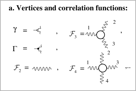
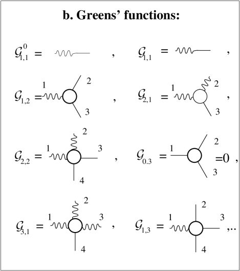
FIG. 1.: The diagrammatic notation of the basic objects of the theory. Panel a: the vertex $\gamma$ and the correlation functions ${\cal F}_{n}$ with $n=2,3,4$. The vertex $\Gamma$ has not been defined yet, but it appears later, cf. Eq. (61). Panel b: the bare Green’s function ${\cal G}^{0}_{1,1}$ (thin line), and the dressed Green’s functions ${\cal G}_{n,m}$. Objects with only straight tails are identically zero.

$C\nu{\bf{\cal J}}_{n,p}(\{{\bf{R}}_{j}\},0)/R_{\rm min}^{2}$ where $C$ is a $\nu$-independent constant and $R_{\rm min}$ is the minimal separation between the coordinates. There is nothing in this quantity to balance $\nu$ in the limit $\nu\to 0$. This is of course the advantage of working with fully unfused quantities; we could not do this with the balance equation for fused correlators [say structure functions $S_{n}(R)$] as the dissipative term approaches a finite limit when $\nu\to 0$. Thus for $\nu\to 0$, or for very large Reynolds numbers, we have

$${\partial{\bf{\cal F}}_{n}({\bf{r}}_{0}|X_{1},\dots,X_{n})\over dt_{1}}+{\bf{\cal D}}_{n}({\bf{r}}_{0}|X_{1},\dots,X_{n})=0\ .$$ (40)

These equations, which are exact, can be written as a chain of equations relating the rate of change of the $n$th order correlation function to the ($n+1$)th order correlation function. To this aim introduce the vertex function

$$\gamma^{\alpha\mu\sigma}({\bf{r}}_{1},{\bf{r}}^{\prime}_{1},\tilde{\bf{r}})={1\over 2}\{[P^{\alpha\mu}({\bf{r}}_{1}-\tilde{\bf{r}})-P^{\alpha\mu}({\bf{r}}^{\prime}_{1}-\tilde{\bf{r}})]{\partial\over\partial\tilde{r}_{\sigma}}$$ (41)

$$+[P^{\alpha\sigma}({\bf{r}}_{1}-\tilde{\bf{r}})-P^{\alpha\sigma}({\bf{r}}^{\prime}_{1}-\tilde{\bf{r}})]{\partial\over\partial\tilde{r}_{\mu}}\ .$$ (42)

With the help of this function we rewrite Eq. (21) in the form

$$[{\partial\over\partial t_{1}}-\nu(\nabla_{1}^{2}+\nabla_{1^{\prime}}^{2})]{\cal W}^{\alpha}({\bf{r}}_{0}|X_{1})$$ (43)

$$+ \int d\tilde{\bf{r}}\gamma^{\alpha\mu\sigma}({\bf{r}},{\bf{r}}^{\prime},\tilde{\bf{r}}){\cal W}^{\mu}({\bf{r}}_{0}|\tilde{X}_{1}){\cal W}^{\sigma}({\bf{r}}_{0}|\tilde{X}_{1})$$ (45)

$$=\int d\tilde{\bf{r}}[P^{\alpha\mu}({\bf{r}}_{1}-\tilde{\bf{r}})-P^{\alpha\mu}({\bf{r}}^{\prime}_{1}-\tilde{\bf{r}})]\phi^{\mu}({\bf{r}}_{0}|\tilde{\bf{r}},t_{1}).$$

Here we used the shorthand notation

$$\tilde{X}_{1}\equiv(\tilde{\bf{r}},{\bf{r}}_{0},t_{1})\ .$$ (46)

From this we can present immediately the interaction term ${\bf{\cal D}}_{n}$ in the hierarchy of equations as follows

$${\cal D}^{\alpha\beta\gamma\dots}_{n}({\bf{r}}_{0}|X_{1},\dots,X_{n})=\int d\tilde{\bf{r}}\gamma^{\alpha\mu\sigma}({\bf{r}}_{1},{\bf{r}}^{\prime}_{1},\tilde{\bf{r}})$$ (47)

$$\times{\cal F}^{\mu\sigma\beta\gamma\dots}_{n+1}({\bf{r}}_{0}|\tilde{X}_{1};\tilde{X}_{1};X_{2},\dots,X_{n+1})\ .$$ (48)

In order to make the structure of these equations more transparent we will represent them graphically using the diagrammatic notations introduced in Fig.1. The convention chosen here is that every velocity difference is represented by a wavy line of unit length, and the 2-point correlator as a wavy line of twice that length. The forcing is represented by a straight line of unit length. Thus the Green’s function, which is the response of the velocity field to the forcing, is represented by a wavy line of unit length connected to a straight line of unit length which represents the forcing. This convention is generalized to the higher order quantities as is evident from Fig. 1. The higher order quantities carry a “junction” that connects the appropriate number of wavy and straight lines of unit length each. The diagrammatic representation of the hierarchy (40) with the interaction term (48) is shown in Fig. 2. The numbers $j=1,2,3,4$ represent sets of coordinates $X_{j}$ together with the corresponding vector indices of the correlation functions ${\bf{\cal F}}_{n}$. The two wavy lines designated by “$\tilde{1}$” are connected to the empty circle ${\bf{\gamma}}$. This means that both these lines carry the same set of coordinates $\tilde{X}_{1}$, and one is supposed to integrate over $\tilde{\bf{r}}$, as is required by Eq. (48).

FIG. 2.: The hierarchy of equation for the correlation functions. The rate of change of ${\cal F}_{n}$ is related to an integral over ${\cal F}_{n+1}$ according to Eqs. (29) and (33). There are two tails designated by $\tilde{1}$, carrying the coordinates $\tilde{X}_{1}$. An integration over $\tilde{r}$ is assumed.

2 The Green’s functions

The equation of motion for the standard Green’s function $G={\cal G}_{1,1}$ of Eq. (29) may be derived straightforwardly. Begin with Eq. (45) for ${\cal W}_{1}^{\alpha}$ and evaluate its functional derivative with respect to $\phi_{2}^{\beta}$. After averaging one gets

$$\Big{[}{\partial\over\partial t_{1}}-\nu(\nabla_{1}^{2}+\nabla_{1^{\prime}}^{2})\Big{]}{\cal G}^{\alpha\beta}_{1,1}({\bf{r}}_{0}|X_{1};x_{2})$$ (49)

$$+\int d\tilde{\bf{r}}\gamma^{\alpha\mu\sigma}({\bf{r}}_{1},{\bf{r}}^{\prime}_{1},\tilde{\bf{r}}){\cal G}^{\mu\sigma\beta}_{2,1}({\bf{r}}_{0}|\tilde{X}_{1},\tilde{X}_{1};x_{2})$$ (50)

$$=G^{(0)\alpha\beta}({\bf{r}}_{1},{\bf{r}}^{\prime}_{1},{\bf{r}}_{2})\delta(t_{1}-t_{2})\ .$$ (51)

The RHS of this equation displays the (zero-time) bare Green’s function of Eq. (30), which consists of a difference between two transverse projection operators:

$$G^{(0)\alpha\beta}({\bf{r}}_{1},{\bf{r}}^{\prime}_{1},{\bf{r}}_{2})=P^{\alpha\beta}({\bf{r}}_{1}-{\bf{r}}_{2})-P^{\alpha\beta}({\bf{r}}^{\prime}_{1}-{\bf{r}}_{2}).$$ (52)

The nonlinear term in the equation of motion (45) results in the appearance of the next-order Green’s function ${\bf{\cal G}}_{2,1}$ in the equation of motion (51). In its turn, the equation of motion of ${\bf{\cal G}}_{2,1}$ will involve the next-order Green’s function ${\bf{\cal G}}_{3,1}$. We begin to build a hierarchy of equations for ${\bf{\cal G}}_{n,1}$ similar to the hierarchy of equations for the correlation functions ${\cal F}_{n}$.

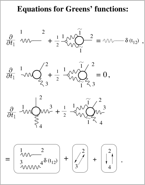
FIG. 3.: The hierarchy of equation for the Green’s functions. The notation is the same as in Fig.2. The two last terms on the RHS of the last equation can be obtained from the first one (in the same frame) by permuting $2\leftrightarrow 3$ and $2\leftrightarrow 4$, as is shown.

To derive this hierarchy we begin again with Eq. (45) for ${\cal W}_{1}^{\alpha}$, multiply the equation by ${\cal W}_{2}^{\beta}\dots{\cal W}_{n}^{\psi}$, and then evaluate the functional derivative with respect to $\phi^{\omega}_{n+1}$. After averaging and discarding the viscous term the resulting equations read

$${\partial\over\partial t_{1}}{\cal G}^{\alpha\beta\dots\psi\omega}_{n,1}({\bf{r}}_{0}|X_{1},X_{2},\dots,X_{n};x_{n+1})$$ (53)

$$+\int d\tilde{\bf{r}}\gamma^{\alpha\mu\sigma}({\bf{r}}_{1},{\bf{r}}^{\prime}_{1},\tilde{\bf{r}})$$ (54)

$$\times{\cal G}^{\mu\sigma\beta\gamma\dots\psi\omega}_{n+1,1}(\tilde{X}_{1},\tilde{X}_{1},X_{2},\dots,X_{n};x_{n+1})$$ (55)

$$={\cal G}_{n,1}^{(0)\alpha\beta\dots\omega}({\bf{r}}_{0}|X_{1},X_{2}\dots X_{n},{\bf{r}}_{n+1},t_{1}+0)\delta(t_{1}-t_{n+1})\ .$$ (56)

The bare Green’s function of $(n,1)$ order on the RHS of this equation are the following decomposition:

$${\cal G}_{n,1}^{(0)\alpha\beta\dots\psi\omega}({\bf{r}}_{0}|X_{1},X_{2}\dots X_{n},{\bf{r}}_{n+1},t_{1}+0)$$ (57)

$$\equiv G^{(0)\alpha\omega}({\bf{r}}_{1},{\bf{r}}^{\prime}_{1},{\bf{r}}_{n+1}){\cal F}^{\beta\gamma\dots\psi}_{n-1}({\bf{r}}_{0}|X_{2},\dots,X_{n-1})\ .$$ (58)

The diagrammatic representation of the first three equations in the hierarchy for ${\bf{\cal G}}_{n,1}$ are shown in Fig. 3. The main difference of this hierarchy from Eqs. (40) is the presence of inhomogeneous terms on the RHS. The second equation in Fig. 3 is atypical in having a zero on the RHS. The origin of this zero is simply the fact that ${\bf{\cal F}}_{1}=0$.

In a similar manner we can derive additional hierarchies of equations for ${\bf{\cal G}}_{n,2}$, ${\bf{\cal G}}_{n,3}$, etc. We do this starting from the same equation of motion (45) for ${\bf{\cal W}}_{1}$, multiplying it by ${\bf{\cal W}}_{2}\dots{\bf{\cal W}}_{n}$, and then evaluating the second order, third order, etc. functional derivative with respect to the forcing. The resulting hierarchy of equations reads

$${\partial\over\partial t_{1}}{\bf{\cal G}}_{n,p}({\bf{r}}_{0}|X_{1},X_{2},\dots,X_{n},x_{n+1},\dots x_{n+p})$$ (59)

$$+\int d\tilde{\bf{r}}{\bf{\gamma}}^{(}{\bf{r}}_{1},{\bf{r}}^{\prime}_{1},\tilde{\bf{r}})$$ (60)

$$\times{\bf{\cal G}}_{n+1,p}({\bf{r}}_{0}|\tilde{X}_{1};\tilde{X}_{1},X_{2},\dots,X_{n};x_{n+1}\dots x_{n+p})$$ (61)

$$=\sum_{j=1}^{p}{\bf{G}}^{(0)}({\bf{r}}_{0}|{\bf{r}}_{1},{\bf{r}}^{\prime}_{1},{\bf{r}}_{n+j})\delta(t_{1}-t_{j}){\bf{\cal G}}_{n-1,p-1}({\bf{r}}_{0}|X_{2}\dots$$ (62)

$$\ \ \ \dots X_{n},{\bf{r}}_{n+1},\dots,{\bf{r}}_{n+j-1},{\bf{r}}_{n+j+1},\dots{\bf{r}}_{n+p})\ .$$ (63)

In this equation the viscous terms have again been discarded; they are vanishingly small in the limit $\nu\to 0$ compared to the other terms in the equations for the fully unfused Green’s functions.

3 The temporal dependence of the statistical quantities: Temporal Multiscaling

In this section we discuss the temporal dependence of our space-time correlation functions, culminating with a new representation for them, see Eq. (83) below. This representation will be very useful in setting up our scheme to compute the scaling exponents. Along the way we will prove the statement that if the strong assumption presented in Eq. (11) were true, than our hierarchy of equations would have predicted a linear dependence of $\zeta_{n}$ on $n$. Our first step then is to show that Eq. (11) is in contradiction with a nonlinear dependences of $\zeta_{n}$ on $n$.

A Locality of the Interaction Integrals

In this subsection we discuss the locality of the integrals appearing in the hierarchic equations (40) and (48), where “locality” here means that the integrals converge in the infrared and in the ultraviolet limits. This property is important, since it excludes the appearance of a renormalization scale as a cutoff on the spatial integrals. Moreover, we will show that the locality of the integrals in addition to the assumption of full scale invariance (7) imply linear scaling. Thus the only way to get anomalous scaling is to show that (7) is incorrect, as we will do in the next section. Fortunately, the property of locality of the integral appearing in (48) was established already in previous publications. It stems from the existence of the fusion rules which govern the asymptotic properties of the correlation functions when a group of coordinates coalesce together [12, 13]. To control the ultraviolet properties of the integrals we need to analyze the situation when the dummy integration coordinate $\tilde{\bf{r}}$ approaches either ${\bf{r}}_{0}$, or any of the other coordinates ${\bf{r}}_{i}$. The asymptotic behavior of the integrand is then determined by the fusion rules for the fusion of two coordinates while all the rest of the coordinates remain separated by much larger distances. The infrared limit is obtained when $\tilde{\bf{r}}\to\infty$, and the asymptotics of the integrand are governed by fusion rules for $n-1$ coordinates coalescing together compared to a single coordinate that approaches an infinite distance from all the rest. Using the fusion rules in this way one can prove convergence in a wide window of the numerical values of the scaling exponents around their K41 or experimental values [13].

B The Consequences of Locality

The differential equations (40) can be turned readily into integral equations by integrating over the time variable. We argued above that the spatial integration converges in the infrared and the ultraviolet regimes. Here we explain the consequences of this property of locality. The needed material was developed in some detail in Ref.[10] but we repeat here all the essentials.

In general our $n$-order correlation functions may depend on $n$ different times. If Eq. (7) were correct, the correlation functions would be a homogeneous function of all the time coordinates. On the other hand, some of these times could be the same, and when they are all the same we get our simultaneous object (7) which is believed to be homogeneous in its spatial coordinates. The simplest many-time case is the one in which there are two different times in (26). Chose $t_{i}=t+s$ for every $i\leq p$ and $t_{i}=t$ for every $i>p$. We will denote the correlation function with this choice of times as ${\bf{\cal F}}_{n,1}^{(p)}(s)$, omitting for brevity the rest of the arguments. Introduce the typical decorrelation time $s_{n,1}^{(p)}(R)$ that is associated with the one-time difference quantity ${\bf{\cal F}}^{(p)}_{n,1}(s)$ when all the spatial separations are of the order of $R$:

$$\int^{\infty}_{0}ds{\bf{\cal F}}^{(p)}_{n,1}(s)\equiv s_{n,1}^{(p)}{\bf{\cal F}}^{(p)}_{n,1}(0)\ .$$ (64)

In Ref.[10] we showed that the consequence of locality is that $s_{n,1}^{(p)}$ satisfies a $p$-independent scaling law:

$$s_{n,1}(R)\sim RS_{n-1}(R)/S_{n}(R)\propto R^{z_{n,1}}\ .$$ (65)

There we introduced the dynamical scaling exponent $z_{n,1}$ that characterizes this time and found that

$$z_{n,1}=1+\zeta_{n-1}-\zeta_{n}\ .$$ (66)

Now we ask whether the same time scale also characterizes correlation functions having two or more time separations. Consider the three-time quantity that is obtained from ${\bf{\cal F}}_{n}$ by choosing $t_{i}=t+s_{1}$ for $i\leq p$, $t_{i}=t+s_{2}$ for $p<i\leq p+q$, and $t_{i}=t$ for $i>p+q$. We denote this quantity as ${\bf{\cal F}}_{n,2}^{(p,q)}(s_{1},s_{2})$, omitting again the rest of the arguments. We define the decorrelation time $s_{n,2}^{(p,q)}$ of this quantity by

$$\int^{\infty}_{0}ds_{1}ds_{2}{\bf{\cal F}}_{n,2}^{(p,q)}(s_{1},s_{2})\equiv[s_{n,2}^{(p,q)}]^{2}{\bf{\cal F}}_{n,2}^{(p,q)}(0,0)\ .$$ (67)

One could think naively that the decorrelation time $s_{n,2}^{(p,q)}$ is of the same order as (65). The calculation [10] leads to a different result:

$$[s_{n,2}(R)]^{2}\sim R^{2}S_{n-2}(R)/S_{n}(R)\propto[R^{z_{n,2}}]^{2}\ .$$ (68)

We see that the naive expectation implied by Eq. (11) is not realized. The scaling exponent of the present time is different from (66):

$$z_{n,2}=1+(\zeta_{n-2}-\zeta_{n})/2\ .$$ (69)

The difference between the two scaling exponents $z_{n,1}-z_{n,2}=\zeta_{n-1}-(\zeta_{n}+\zeta_{n-2})/2$. This difference is zero for linear scaling, meaning that in such a case the naive expectation that the time scales are identical is correct. On the other hand for the situation of multiscaling the Hoelder inequalities require the difference to be positive. Accordingly, for $R\ll L$ we have $s_{n,2}(R)\gg s_{n,1}(R)$.

We can proceed to correlation functions that depend on $m$ time differences. Omitting the upper indices which are irrelevant for the scaling exponents we denoted [10] the correlation function as ${\bf{\cal F}}_{n,m}(s_{1}\dots s_{m})$, and established the exact scaling law for its decorrelation time. The definition of the decorrelation time is

$$\int^{\infty}_{0}ds_{1}\dots ds_{m}{\bf{\cal F}}_{n,m}(s_{1}\dots s_{m})\equiv[s_{n,m}]^{m}{\bf{\cal F}}_{n,m}(0\dots 0).$$ (70)

We found the dynamical scaling exponent that characterizes $s_{n,m}$ when all the separations are of the order of $R$, $s_{n.m}\propto R^{z_{n,m}}$:

$$z_{n,m}=1+(\zeta_{n-m}-\zeta_{n})/m\ ,\quad n-m\leq 2.$$ (71)

One can see, using the Hoelder inequalities, that $z_{n,m}$ is a nonincreasing function of $m$ for fixed $n$, and in a multiscaling situation they are decreasing. The meaning is that the larger is $m$, the longer is the decorrelation time of the corresponding $m+1$-time correlation function, $s_{n,p}(R)\gg s_{n,q}(R)\ \ {\rm for}\ \ p<q\$.

It is obvious now that the assumption of complete scale invariance (11), which is tantamount to the assertion that $z_{n,m}$ is $m$-independent, necessarily requires a linear dependence of $\zeta_{n}$ on $n$. An $m$-independent $z_{n,m}$ means that

$$\zeta_{n-m}-\zeta_{n}={\rm const}\times m\ ,\quad{\rm linear~{}scaling!}\ .$$ (72)

The results (71) shows that in a multi-scaling situation our correlation functions cannot exhibit scale invariance.

To expose the consequences in a complementary way that will be useful in what follows, we considered higher order temporal moments of the two-time correlation functions:

$$\int^{\infty}_{0}dss^{k-1}{\bf{\cal F}}^{(p)}_{n,1}(s)\equiv({\overline{s^{k}}})^{(p)}_{n,1}{\bf{\cal F}}^{(p)}_{n,1}(0)\ .$$ (73)

The intuitive meaning of $({\overline{s^{k}}})^{(p)}_{n,1}$ is a $k$-order decorrelation moment of ${\bf{\cal F}}^{(p)}_{n,1}(R,s)$ whose dimension is (time)^k. The first order decorrelation moment is the previously defined decorrelation time $s_{n,1}^{(p)}$. We found the scaling laws

$$[\overline{s^{k}}]_{n,1}^{(p)}\sim(s_{n,k})^{k}\sim R^{k}S_{n-k}(R)/S_{n}(R)$$ (74)

for $k\leq n-2$. The procedure does not yield information about higher $k$ values. We learn from the analysis of the moments that there is no single typical time which characterizes the $s$ dependence of ${\bf{\cal F}}^{(p)}_{n,1}$. There is no simple “dynamical scaling exponent” $z$ that can be used to collapse the time dependence in the form ${\bf{\cal F}}^{(p)}_{n,1}(s)\sim R^{\zeta_{n}}f(s/R^{z})$. Even the two-time correlation function is not a scale invariant object. In this respect it is similar to the probability distribution function of the velocity differences across a scale $R$, for which the spectrum of exponents $\zeta_{n}$ is a reflection of the lack of scale invariance.

C Temporal Multiscaling Representation

This subsection offers a convenient presentation of the time dependence of the correlation functions. Consider first the simultaneous function ${\bf{\cal T}}_{n}({\bf{r}}_{1}\dots{\bf{r}}^{\prime}_{n})$. Following the standard ideas of multifractals [4, 20] the simultaneous function can be represented as

$${\bf{T}}_{n}({\bf{r}}_{1},{\bf{r}}^{\prime}_{1}\dots{\bf{r}}^{\prime}_{n})=U^{n}\int_{h_{\rm min}}^{h_{\rm max}}d\mu(h)\left({R_{n}\over L}\right)^{nh+{\cal Z}(h)}$$ (75)

$$\times\tilde{T}_{n,h}({\bf{\rho}}_{1},{\bf{\rho}}^{\prime}_{1},\dots,{\bf{\rho}}^{\prime}_{n})\ .$$ (76)

Here $U$ is a typical velocity scale, and we have introduced the “typical scale of separation” of the set of coordinates

$$R^{2}_{n}={1\over n}\sum_{j=1}^{n}|{\bf{r}}_{j}-{\bf{r}}_{j}^{\prime}|^{2}\ .$$ (77)

Greek coordinates stand for dimensionless (rescaled) coordinates, i.e.

$${\bf{\rho}}_{j}={\bf{r}}_{j}/R_{n}\ ,\quad{\bf{\rho}}^{\prime}_{j}={\bf{r}}^{\prime}_{j}/R_{n}\ ,\$$ (78)

and finally the function ${\cal Z}(h)$ is defined as

$${\cal Z}(h)\equiv 3-{\cal D}(h)\ .\$$ (79)

The function ${\cal Z}(h)$ is related to the scaling exponents $\zeta_{n}$ via the saddle point requirement

$$\zeta_{n}=\min_{h}[nh+{\cal Z}(h)]\ .\$$ (80)

This identification stems from the fact that the integral in (76) is computed in the limit $R_{n}/L\to 0$ via the steepest descent method. Neglecting logarithmic corrections one finds that ${\bf{\cal F}}_{n}\propto R_{n}^{\zeta_{n}}$.

The physical intuition behind the representation (76) is that there are velocity field configurations that are characterized by different scaling exponents $h$. For different orders $n$ the main contribution comes from that value of $h$ that determines the position of the saddle point in the integral (76).

There is no reason why not to extend this intuition to the time domain. The particular velocity configurations that are characterized by an exponent $h$ also display a typical time scale $t_{R,h}$ which is written as

$$t_{R,h}\sim{R\over U}\left({L\over R}\right)^{h}\ .$$ (81)

Accordingly we propose a new temporal multiscaling representation for the time dependent function

$${\bf{\cal F}}_{n}({\bf{r}}_{0}|X_{1},\dots,X_{n})=U^{n}\int\limits_{h_{\rm min}}^{h_{\rm max}}d\mu(h)\left({R_{n}\over L}\right)^{nh+{\cal Z}(h)}$$ (82)

$$\times\tilde{\bf{\cal F}}_{n,h}({\bf{r}}_{0}|\Xi_{1},\Xi_{2},\dots\Xi_{n})\ .$$ (83)

The function $\tilde{\bf{\cal F}}_{n,h}$ depends on dimensionless (rescaled) coordinates

$$\Xi_{j}\equiv({\bf{\rho}}_{j},{\bf{\rho}}^{\prime}_{j},\tau_{j})\ ,\quad\tau_{j}=t_{j}/t_{R_{n},h}\ .$$ (84)

Of course, we require that the function $\tilde{\bf{\cal F}}_{n,h}({\bf{r}}_{0}|\Xi_{1},\dots\Xi_{n})$ is identical to $\tilde{T}_{n,h}({\bf{\rho}}_{1},{\bf{\rho}}^{\prime}_{1},\dots,{\bf{\rho}}^{\prime}_{n})$ when its rescaled time arguments are all the same.

The point of this presentation is that it reproduces all the scaling laws that are involved in time integrations and differentiations. For example, specializing to the case of one time difference as discussed in Section 4, we can perform the integral appearing in Eq. (73), and derive immediately the result in (74).

4 Setting up a calculation of the scaling exponents

This section contains the main result of this paper, i.e. the equations that we propose as the starting point for the calculation of the scaling exponents.

One of the main insights gained by understanding the temporal properties of the correlation functions is that it is not true that the hierarchy of equations for the correlation functions dictate classical scaling by power counting. The way to see this is to substitute the temporal multiscaling representation (83) in the hierarchy of equations (48), and see that power counting gives no information:

$$\int_{h_{\rm min}}^{h_{\rm max}}d\mu(h)\left({R_{n}\over L}\right)^{(n+1)h+{\cal Z}(h)}\Big{\{}{\partial\over\partial\tau_{1}}\tilde{\bf{\cal F}}_{n,h}(\Xi_{1},\dots,\Xi_{n})$$ (85)

$$+\int d\tilde{\bf{\rho}}{\bf{\gamma}}({\bf{\rho}}_{1},{\bf{\rho}}_{2},\tilde{\bf{\rho}})\left({R_{n+1}\over R_{n}}\right)^{(n+1)h+{\cal Z}(h)}$$ (86)

$$\times\tilde{\bf{\cal F}}_{n+1,h}(\tilde{\Xi},\tilde{\Xi},\Xi_{2},\dots\Xi_{n})\Big{\}}=0\ .$$ (87)

In this equation $R_{n+1}$ is the mean scale of separation of the $2(n+1)$ space coordinates of the function ${\bf{\cal F}}_{n+1}$ similarly to (77). This set of equations can be considered as a linear set of functional equations for the structure functions in rescaled coordinates. Since this equation has to be valid for any value of $L$, and since we integrate over a positive measure, the equation is satisfied only if the terms in curly parentheses vanish. In other words, we will seek solutions to the equations

$${\partial\over\partial\tau_{1}}\tilde{\bf{\cal F}}_{n,h}(\Xi_{1},\dots,\Xi_{n})+\int d\tilde{\bf{\rho}}{\bf{\gamma}}({\bf{\rho}}_{1},{\bf{\rho}}_{2},\tilde{\bf{\rho}})$$ (88)

$$\times\left({R_{n+1}\over R_{n}}\right)^{(n+1)h+{\cal Z}(h)}\tilde{\bf{\cal F}}_{n+1,h}(\tilde{\Xi},\tilde{\Xi},\Xi_{2},\dots\Xi_{n})=0\ .$$ (89)

We note the important fact that this equation is invariant to the rescaling

$${\bf{r}}_{i}\to\lambda{\bf{r}}_{1}\ ,\quad t_{i}\to\lambda^{1-h}t_{i}\ ,$$ (90)

for any value of $\lambda$ and $h$. Accordingly, power counting leads to no result. As a consequence the information about the scaling exponents $\zeta_{n}$ is obtainable only from the solvability conditions of this equation. In other words, the information is buried in coefficients rather than in power counting. The spatial derivative in the vertex on the RHS brings down the unknown function ${\cal Z}(h)$, and its calculation will be an integral part of the computation of the exponents.

We recognize nevertheless that this set of equations forms an infinite hierarchy. To proceed we need to find intelligent ways to truncate the hierarchy without reintroducing power counting. To this aim we are going to use renormalized perturbation theory, which is one of the best schemes available to express higher order quantities in terms of lower order ones. We review the needed material in the next section.

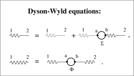
FIG. 4.: The coupled Dyson (first line) and Wyld (second line) equations for the Green’s functions and second order correlator respectively. The mass operators are displayed in Fig. 5

5 Resummations in successive orders

In this section we discuss successive resummations of renormalized perturbation theory. In doing so we will demonstrate that the theory generates infinitely many renormalized objects whose scaling properties are non-trivial. The first step is the standard line-resummation that produces renormalized two-point functions. Further resummations produce three-, four-, and higher point renormalized objects. We prove that this procedure generates equations that in their fully resummed form are identical in content to the exact hierarchies of equations derived above directly from the fluid equations of motion. Next we explain how partially resummed versions can be used to offer controlled approximations to the full calculation.

Equation (45) can be used as a starting point for the development of a line-renormalized perturbation theory for the statistical quantities. The reader should note that this equation is slightly different than the one used previously [14] for the same purpose. The difference is that previously one used an equation for a quantity that in the present notation reads ${\bf{\cal W}}({\bf{r}}_{0}|{\bf{r}},{\bf{r}}_{0},t)$. Accordingly, one cannot read blindly the results of the previous analysis. Nevertheless the differences are not serious, and the spirit is the same as before.

The diagrammatic representation of the Dyson-Wyld equations for the Green’s function ${\bf{\cal G}}_{1,1}$ and the second order correlation function ${\bf{\cal F}}_{2}$ is identical to its previous counterpart [14], and shown in Fig. 4. In symbols the Dyson equation reads now

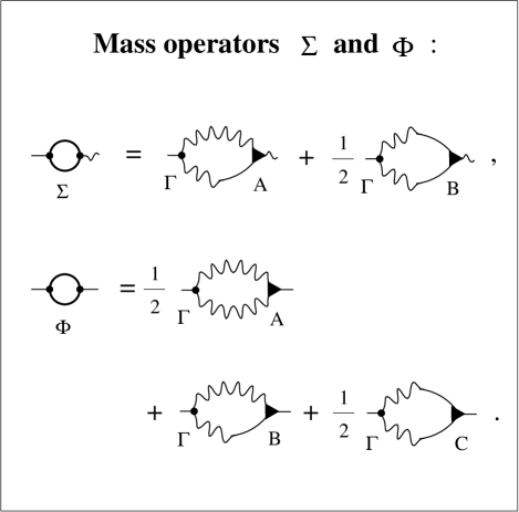
FIG. 5.: Exact representations of the mass operators $\Sigma$ and $\Phi$ in terms of the bare vertex $\Gamma$, the Green’s function and second order correlator, and the dressed three-legged vertices A,B,C.

$${\cal G}^{\alpha\beta}_{1,1}({{\bf{r}}}_{0}|X_{1};x_{2})={\cal G}^{(0)\alpha\beta}_{1,1}({{\bf{r}}}_{0}|X_{1};x_{2})$$ (91)

$$+\int d{{\bf{r}}}_{a}\int_{t_{2}}^{t_{1}}dt_{a}{\cal G}^{(0)\alpha\delta}_{1,1}({{\bf{r}}}_{0}|X_{1};x_{a})$$ (92)

$$\times\int d{{\bf{r}}}_{b}\int_{t_{2}}^{t_{a}}dt_{b}\Sigma^{\delta\gamma}({{\bf{r}}}_{0}|{{\bf{r}}}_{a},{{\bf{r}}}_{b},t_{a}-t_{b}){\cal G}^{\gamma\beta}_{1,1}({{\bf{r}}}_{0}|\tilde{X}_{b},x_{2})\ ,$$ (93)

where $\tilde{X}_{b}=\{{\bf{r}}_{b},{\bf{r}}_{0},t_{b}\}$. One sees that the number 1 designates a set of coordinates $X_{1}$ and a corresponding vector index $\alpha$, the number 2 corresponds to $X_{2}$ and a corresponding vector index $\beta$. The meaning of “a” is evident from the comparison of Eq. (92) with the first line of Fig. 4. The Wyld equation for the 2nd order correlation function has the form

$${\cal F}^{\alpha\beta}_{2}(B.r_{0}|X_{1},X_{2})=\int d{{\bf{r}}}_{a}d{{\bf{r}}}_{b}\int_{t_{1}}^{\infty}dt_{a}\int_{t_{2}}^{\infty}dt_{b}$$ (94)

$$\times {\cal G}^{\alpha\delta}_{1,1}({{\bf{r}}}_{0}|X_{1};x_{a}){\cal G}^{\beta\mu}({{\bf{r}}}_{0}|X_{2};x_{b})\Phi^{\delta\mu}({{\bf{r}}}_{0}|x_{a},x_{b})\ .$$ (95)

The meaning of $1,2,a$ and $b$ is again evident after comparing the second line of Fig. 4 with Eq. (95). In equation (92) the “mass operator” $\Sigma$ is related to the “eddy viscosity” whereas in Eq. (95) the “mass operator” $\Phi$ is the renormalized “nonlinear” noise which arises due to turbulent excitations. Both these quantities are given as infinite series in terms of the Green’s function and the correlator, and thus the equations are coupled. The diagrammatic notation for the vertex $\Gamma$ is presented in Fig. 1a. Analytically $\Gamma_{\alpha\beta\gamma}({\bf{r}})$ is a local differential operator of the Euler equation

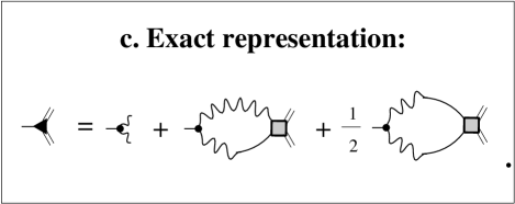
FIG. 6.: The 3rd order vertices. Panel a: The three different types of 3rd order vertices, A, B, and C. A double lined tail stands for either wavy or straight tail. There is no vertex with three wavy tails in the theory. Panel b: The diagrammatic representation of a dressed 3rd order vertex (A, B or C) as an infinite series in terms of dressed 3rd order vertices and propagators. There is only one type of bare vertex appearing in the series for the dressed vertex A. Panel c: The exact representation of 3rd order vertices in terms of the partly reducible 4th order vertex (gray square) which is defined in Fig. 7.

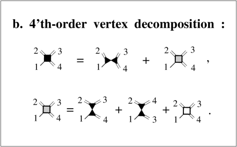
FIG. 7.: The 4th order vertices. Panel a: the different types of 4th order vertices. A double lined tail stands for either wavy or straight tail, see text. Panel b, first line: decomposition of 4th order vertices in terms of partly reducible contributions (gray square). Panel b, second line: further decomposition of the vertex into two-eddy reducible parts and fully irreducible 4the order vertices (emplty square). The latter are shown in Fig. 13. Panels c and d: Skeleton contributions to the 4th order vertices. There are three terms in Panel d with three types of propagators. There is just one term in Panel c, the two other type of propagators require a tripple vertex with three wavy tails which is zero.

$$\Gamma^{\alpha\beta\gamma}({\bf{r}})=-(\delta_{\alpha\gamma}\nabla_{\beta}+\delta_{\alpha\beta}\nabla_{\gamma})\ .$$ (96)

which is different from the non-local bare vertex ${\bf{\gamma}}$, Eq. 42. This vertex is related to ${\bf{\Gamma}}$ via the bare Green’s function (52) where $G^{(0)\alpha\beta}$ is given by Eq. (52):

$$\gamma^{\alpha\beta\gamma}({\bf{r}}_{1},{\bf{r}}^{\prime}_{1},{\bf{r}}_{2})=-G^{(0)\alpha\delta}({{\bf{r}}}_{1},{\bf{r}}^{\prime}_{1},{{\bf{r}}}_{2})\Gamma^{\delta\beta\gamma}({\bf{r}}_{2})\ ,$$ (97)

where only the repeated tensor index $\delta$ is summed upon. The bare Green’s function in the BL-representation satisfies the equation

$$\Big{[}{\partial\over\partial t_{1}} - \nu\big{(}\nabla^{2}_{1}+\nabla^{2}_{1^{\prime}}\big{)}\Big{]}{\cal G}_{1,1}^{(0)\alpha\beta}({{\bf{r}}}_{0}|X_{1},x_{2})$$ (98)

$$= G^{(0)\alpha\beta}({\bf{r}}_{1},{\bf{r}}^{\prime}_{1},{\bf{r}}_{2})\delta(t-t_{2})\ ,$$ (99)

The series for ${\bf{\Sigma}}$ and ${\bf{\Phi}}$ can be resummed exactly, as is shown in Fig. 5. There is a price to pay: there are three new objects that appear as a result of this resummation, known as the ‘triple” vertices A, B and C. They differ in the number of wavy tails that connect them to the propagators. Note that there is no triple vertex with three wavy tails; such a vertex vanishes due to causality, as is discussed in Appendix A. Each of these vertices can be represented as an infinite series in terms of the same objects, i.e. the vertices A,B,C, and the correlator and propagator. The first diagrams in the infinite series for the triple vertices are shown in Fig. 6b.

In fact one is not limited to an infinite series representation. One can also represent the triple vertices through exact and complete resummations of the infinite series, but this is at the expense of introducing yet another set of objects, this time of quartic nature. There are four different quartic vertices, with one, two, three or four straight “legs”. We denote them as $D_{m.n}$ with $m$ standing for the number of wavy tails, and $n$ for the number of straight tails, $m+n=4$. It is natural to discuss the various contributions appearing in these objects as “skeleton” and “irreducible” and this discussion is presented in Appendix A.

This process goes on. We can offer an exact, fully resummed equation for the quartic vertices, but at the price of introducing quintic objects,etc, as is explained in detail in Appendix A. The renormalized vertices serve also in providing exact representations for the many-point different-time correlation functions (5). As examples we present in Figs.8,9 the exact and fully renormalized three-point correlation function ${\bf{\cal F}}_{3}$ and the nonlinear Green’s function ${\bf{\cal G}}_{2,1}$ in terms of the double correlator, the Green’s function and the triple vertices.

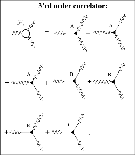
FIG. 8.: Exact representation of the third-order correlation function.

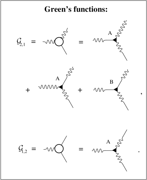
FIG. 9.: Exact representation of the nonlinear Green’s functions ${\cal G}_{2,1}$ and ${\cal G}_{1,2}.$

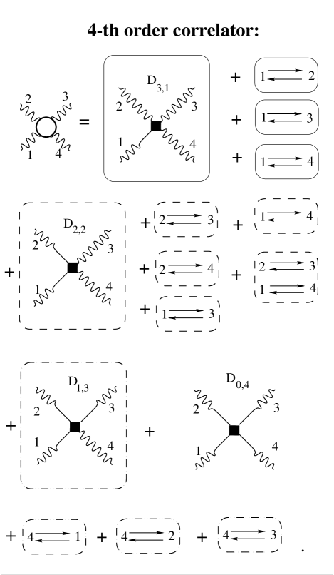
FIG. 10.: Exact representation of the 4th-order correlation function ${\cal F}_{4}$ in terms of 4th order vertices (black squares) and propagators. The meaning of the 4th order vertex is discussed in Appendix A. The notation in this figure is that every contributions that is shown explicitly in a frame adds up to the indicated permutations enclosed in frames of the same line type.

Similarly we can provide an exact representation of the four point correlation function ${\bf{\cal F}}_{4}$ in terms of the same two-point correlator and Green’s function and the quartic vertices shown in Fig. 10. And so on; ${\bf{F}}_{n}$ can be represented as $2^{n}-1$ contributions in terms of n-legged vertices.

We see that we have a theory that allows exact representations of as many renormalized objects as we desire. It appears clear and elegant, but in fact is almost contentless. In order to endow it with predictive power we need to learn how to perform two tasks. Firstly, the space-time integrals are implicit in every diagram, see for example Eqs. (92,95). We need to learn how to compute them. Secondly, we cannot deal with an infinite hierarchy, and we need to learn how to close the hierarchy efficiently. In the next section we review briefly the past history of attempts to solve these equations, and why they failed in finding anomalous scaling. This will serve as a guidance for the new ideas that pave the route that is taken in the rest of this paper.

6 Why is the Problem Still Open?

The first serious attempt to derive the scaling exponents of the statistical objects was due to Kraichnan [21, 22], who introduced the “Direct-Interaction Approximation” (DIA). In the context of our presentation this approximation means truncating the set of exact equations by replacing the dressed vertex A by its bare counterpart, and by equating the dressed vertices B and C to their bare value which is zero. This approximation leads to closed equations in terms of the second order correlation functions and Green’s function. Kraichnan was the first to understand that after an appropriate transformation of the velocity field (he chose Lagrangian, but Belinicher and L’vov showed that their transformation amounted to the same result) the space integrals in the DIA converge at both ends. As a result of this “locality” of the integrals, neither an inner nor an outer scale appears in the bulk of the inertial interval. In addition, Kraichnan assumed that the space-time correlation functions are scale invariant in the sense of Eq. (11). This assumption, together with the property of locality, lead to the existence of scaling relations connecting the exponents $\zeta_{2}$ and $z$:

$$\zeta_{2}+2z = 2\,,$$ (100)

$$2\zeta_{2}+z = 2\ .$$ (101)

Of course, the solution is K41, i.e. $\zeta_{2}=z=2/3$. It should be understood at this point that this disappointing result will continue to hold not just at the DIA level, but at any finite order in the dressing of the vertex via the perturbative scheme. Since it was shown that every diagram exhibits locality, the scaling relations are reproduced by any finite truncation of the line resummed perturbation theory. Whenever we have a set of linear scaling relations, K41 can be the only solution. It is always a solution by dimensional reasoning, and therefore it must solve any set of scaling relations. The linearity of the scaling relations is then the end of the story.

One way out would be to assert that a full dressing of the vertex may result in a new scaling exponent for that object. We still have a linear set of two scaling relations, but now three exponents to determine. The extra freedom allows deviations from K41. However, this is not the case as long as we believe that the scale invariance as assumed in the form Eq. (11) indeed holds. It was shown by L’vov and Lebedev [23] that under that assumption the exponent of the vertex is unchanged from its bare value of $-1$. Accordingly, K41 seems a deeper trap than ever. Is there a way out?

Our contention is that the fundamental fallacy is the assumption Eq. (11). One could think that there is a fundamental problem with renormalized perturbation theory since the problem lacks a small parameter. To show that this is not the case we develop the theory further, and show that the fully renormalized equations obtained from resumming the diagrammatic expansions are exact and equivalent to hierarchical equations that stem from the Navier-Stokes equations. We will then argue that finite resummations of the perturbation theory up to a given order will give successive approximations which are useful for the solution of the fundamental equations (88).

7 Equivalence of the fully renormalized diagrammatics and the exact hierarchical equations

The student of fluid mechanics who is not familiar with field theoretic methods may find the diagrammatic expansion discussed in section 5 somewhat foreboding. The student of field theories, on the other hand, may find them suspicious since the problem does not have a small parameter. It is important therefore for general understanding, and also crucial for the further development of our theory, to show that the fully resummed equations discussed above are equivalent to hierarchies of equations that can be derived exactly from the Navier-Stokes equations.

Consider first the Dyson equations (92). Applying to this equation the operator $\Big{[}{\partial\over\partial t}-\nu(\nabla^{2}+\nabla_{0}^{2})\Big{]}$ from the left, and using Eq. (98) we can write, in the limit $\nu\to 0$,

$${\partial\over\partial t_{1}}{\cal G}^{\alpha\beta}_{1,1}({{\bf{r}}}_{0}|X_{1};x_{2})=G^{(0)\alpha\beta}({{\bf{r}}}_{1},{{\bf{r}}}^{\prime}_{1},{\bf{r}}_{2})\delta(t_{1}-t_{2})$$ (102)

$$+\int d{{\bf{r}}}_{b}\int_{t_{2}}^{t_{1}}dt_{b}\tilde{\Sigma}^{\alpha\gamma}({{\bf{r}}}_{0}|X_{1};x_{b}){\cal G}_{1,1}^{\gamma\beta}({{\bf{r}}}_{0}|X_{b};x_{2})\ ,$$ (103)

where

$$\tilde{\Sigma}^{\alpha\gamma}({{\bf{r}}}_{0}|X_{1};x_{b})=\int d{{\bf{r}}}_{a}G^{(0)\alpha\delta}({\bf{r}}_{1},{\bf{r}}^{\prime}_{1},{\bf{r}}_{a})$$ (104)

$$\times\Sigma^{\delta\gamma}({{\bf{r}}}_{0}|{{\bf{r}}}_{a},{{\bf{r}}}_{a},t_{1};x_{b})\ .$$ (105)

Next one might compare Fig. 11 with the exact representation of the Green’s function ${\bf{\cal G}}_{2,1}$ which is presented in Fig. 9. The last term in Fig. 11 is obviously a vertex integrated against the last contribution to ${\bf{\cal G}}_{2,1}$ with the B vertex, with a factor of $1/2$. The second term is just the vertex integrated against the other two contributions with vertex A, and in total we retrieve exactly the first equation in the hierarchy presented in Fig. 3.

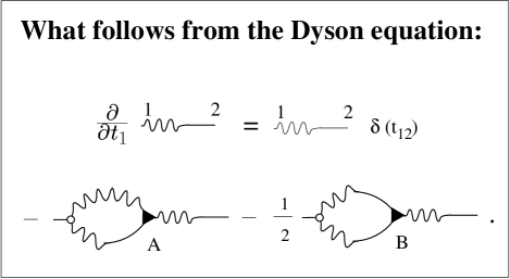
FIG. 11.: The Dyson equation written in terms of the fully resummed vertices A and B.

Figure 12 is a flow chart of the derivation of the first of the hierarchy of equations for the correlation functions. The first equation, denoted by 1 over the equal sign, is obvious. The second one, denoted by 2, is obtained using the Wyld equation (which is the second of Fig. 4). Note that the time derivative is applied only to the Green’s function on the left. Equality 3 is a substitution of the derivative of the Green’s function from Fig. 11. The bare Green’s function (the first term in Fig. 11 changes the dark circle to minus an empty one, in accordance with Eq(97)). One recognizes next that the pieces in the two frames designated $c_{1}$ are the 2nd order correlation function, shown in the frame $c_{2}$. The first term shown in frame $b_{1}$ becomes the three contributions shown in frame $b_{2}$ in panel b by using the exact representation of ${\bf{\Phi}}$ shown in Fig. 5 and relationship between vertices $\Gamma$ and $\gamma$. Lastly, the equation in panel b contains all the contributions to the RHS, which are nothing but the vertex integrated against the 3rd order correlation function, as can be checked by comparing with Fig. 8. We have thus derived the first of the exact hierarchy of equations for the correlation functions shown as the first line of Fig. 2. One can proceed similarly to derive the second of the hierarchic equations for the correlation functions. The starting point would be the exact representation of ${\bf{\cal F}}_{3}$ in Fig. 8. Taking the time derivative with respect to $t_{1}$ one gets seven contributions, four of which involve derivative of the Green’s function ${\bf{\cal G}}_{1,1}$, and three a derivative of ${\bf{\cal F}}_{2}$. For every such derivative we need to substitute either the three terms appearing in Fig. 11, or the five terms appearing in Fig. 12. Special attention should be paid to the contribution of the first term (the bare Green’s function) in Fig. 11. When it is attached to one of the dressed vertices A, B or C one needs to use their exact representation as shown in Figs.6c. In all the other contributions we can leave the dressed vertices A, B and C unchanged. At this point we can collect all the terms, and find 60 terms (counting each one with a factor 1/2 once and with a factor 1 twice). One may then substitute the exact representation for the dark 4th order vertices as a sum of four contributions, like those shown in Fig. 13b in Appendix A. This will reduce the number of contributions to 15, all with dark 4th order vertices. This is precisely the right number of contributions needed to reproduce the exact result which is the empty circle vertex ${\bf{\gamma}}$ integrated against the 15 contributions in ${\bf{\cal F}}_{4}$ shown in Fig. 10. This completes the derivation of the second equation in the hierarchy shown in Fig. 2. Exactly the same procedure (but with fewer terms) provides the derivation of the second equation in the hierarchy of the Green’s function ${\bf{\cal G}}_{n,1}$ shown in Fig. 3 etc.

This derivation can be repeated at any order, showing the exact correspondence of the fully resummed diagrammatics and the hierarchic equations. Since the proof calls for the introduction of additional graphical notations we present it in the appendix for the consideration of the dedicated reader.

The summary of this section is as follows: The classical Dyson-Wyld equations are equivalent to the first equations in the hierarchy of equations for the correlation and Green’s functions. At this step of resummation the 3rd order objects are given only in terms of an infinite series in the 2nd order objects. If we replace at this point the triple vertex by its bare value we will generate the Direct Interaction Approximation. In the next step of resummation we have 2nd and 3rd order objects in fully resummed form. In particular the 3rd order vertices are not given in terms of infinite series but they are exactly represented in a fully resummed form in terms of 4th order objects as shown in Fig. 6c. At this stage we can show agreement with the first two equations of the hierarchies. The 4th order objects are still presented in terms of an infinite series in terms 2nd and 3rd order objects, and one can discuss various ways of approximating the 4th order objects. But one can make instead the next step of resummation, that will yield fully resummed 4th order objects in terms of 5th order ones, see Fig. 13. The 5th order objects are represented at this stage as an infinite series in terms of lower order objects. At this step we can recover the first three equations of the hierarchies. This procedure can be continued to any desired order, and at every $n$-th step of the procedure in which we have fully resummed $n$-order objects, we can recover the first $n-1$ equations of the hierarchies. It is reasonable to assume that by deferring the closure approximation to higher and higher order steps of the resummation we may find better and better answers for the lower order objects. In the next Section we will discuss several possibilities of making intelligent closures.

8 closure schemes

In this section we explain why partly resummed perturbation expansions are useful in implementing intelligent closures of the infinite hierarchy (88). We take as an example a closure at the level of the 3-point vertices A, B and C, but the comments are relevant for closures at higher order as well. The complete discussion belongs to the forthcoming paper [15], and here we just briefly sketch the important ideas, to underline why we spent so much effort on the development of the resummed perturbation theory in Sects. 5-7.

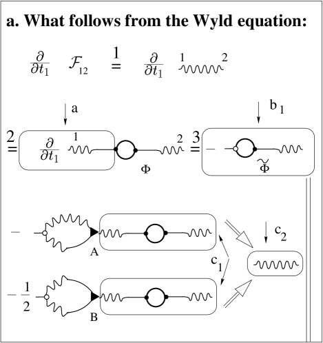
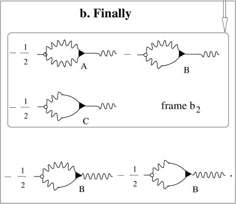
FIG. 12.: Flow chart describing the diagrammatic derivation of the first equation in the hierarchy of equations for the correlation functions.

The main point is that we want to select the closure approximation such as not to reintroduce power counting into the hierarchy (88). Consider then the three point vertices A, B and C. We have for each of these vertices an infinite series in terms of themselves and the lower order 2-point correlation functions and Green’s functions, see Figs.6b. Of course, taking all the infinite contributions is impossible, and we need a criterion to choose partial series of contributions as the approximation for the 3rd-order vertices. One traditional approximation that one could use is the so-called “triangular approximation” [24]; this means that we take all the triangular diagrams like the first four contributions after the bare vertex in Fig. 6b. Each of these triangular diagrams contains three dressed 3-point vertices of type A, B or C, and three propagators (2-point correlator or Green’s function). These diagrams result from the infinite (partial) resummation of all the “planar” diagrams which do not contain crossed lines of propagators. Note that the four shown triangular diagrams are not all the diagrams of this type, but their number is small (for example six in the case of vertex A).

In fact such an approximation is not suitable for our needs. In the forthcoming paper [15] we will show that this approximation reintroduces power counting to the hierarchy (88). On the other hand we will show that the approximation that is obtained by taking only the skeleton contributions and neglecting the fully irreducible contributions is appropriate, since it does not reintroduce power counting. In other words we can use exact representations for the $n$-order fully irreducible vertices in terms of partly reducible $n+1$-order vertex (as shown in Fig. 6 for 3’rd-order vertex and in Fig. 13 for the 4th order vertex) and then to neglect the fully reducible contribution (empty objects) for $n+1$-order vertex in order to select that appropriate infinite partial resummation that does not clash with the rescaling symmetry (12) that we want to preserve. This will be shown and utilized in the forthcoming paper [15]. In particular we will show that when we neglect the fully irreducible contributions to the 4th order vertex we get closed nonlinear equations for the triple vertices as shown in Figs.6c and 7. By neglecting the fully irreducible contributions to the 5th order vertex (see Figs. 14b as and example) we find closed equations for the full 3rd and 4th order vertices, and so on.

9 Appendix A: Discussion of the 4th and the 5th order vertices

There are four types of 4th order vertices, as shown in Fig. 7a. The various contributions to the 4th order vertices are grouped according to their topology in three classes as shown in Fig. 7b. The first class is known as “two-eddy reducible” or “skeleton” contributions. Such contributions, denoted by joint triangles, can be split into two pieces by cutting off one propagator, see panels c and d. The second class is known as “irreducible”, and is denoted as an empty square. The grey square is the third class, termed ”partly reducible”, and made of the irreducible vertex and the reducible contributions. The need to consider separately the grey vetex stems from its appearance in the exact representation of the third order vertices, see Fig.6. All the possible types of skeleton contributions to the 4th order vertices are shown in Figs.7. The diagrammatic notation of the skeleton contribution is a mnemonic to stress the fact that they consist of two dressed triple vertices which were denoted as black triangles. The joining at the apex hides a bridge that can be made from any of the available propagators, either a correlator with a wavy line, or a Green’s function with a straight-wavy line with either orientation. All these terms are presented in Fig. 7d. In contrast, Fig. 7c have only one type of propagator, with the straight line on the right. The two other possibilities have wavy lines on the right, and this requires a 3’rd order vertex with three wavy tails which is zero identically. Note that the line resummed theory does not have bridges made of two consecutive propagators with something in between: such contributions are “one-eddy reducible”, and all such diagrams have been already resummed in the Dyson line resummation.

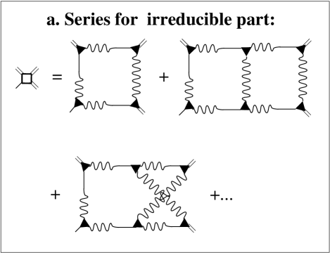
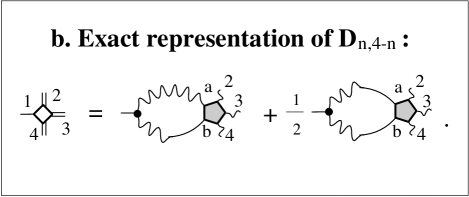
FIG. 13.: Panel a: diagrammatic expansion of the quartic dressed vertices in terms of triple dressed vertices A, B, and C, and propagators. Panel b. Exact representation of the irreducible part of $D_{n,4-n}$ via the partly reducible 5th order vertices shown in Fig 14b.

As noted, the skeleton diagrams are “two-eddy reducible” in the sense that they can be split into two pieces by cutting across the bridge. Examples of irreducible diagrams for $D_{n,4-n}$ which cannot be cut this way are shown in Fig. 13a. There are infinitely many of them. Again, this kind of series can be resummed exactly, as is shown in Fig. 13b. The price is the appearance of an $(n+1)$’th order vertex, 5th order in the present case. This vertex is denoted as a grey pentagon. We will call it “partly reducible” vertex. Consider now 5th order vertices, for example $D_{4,1}$, see Fig. 14. As discussed above we distinguish here the reducible contribution which is explicitly shown in Fig .14a and the partly reducible contribution, shown as gray pentagon. The need to use a special notation (grey pentagon) for the partly reducible vertex is again motivated by its appearance in the exact representatin of the 4th order vertex, Fig.13b. Its further decomposition into reducible parts and a fully irreducible term (empty pentagon) is shown in Fig .14b.

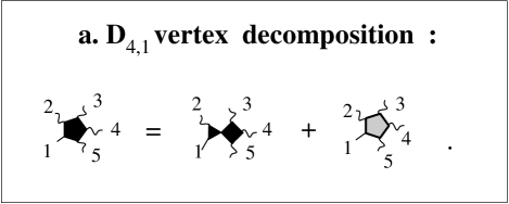
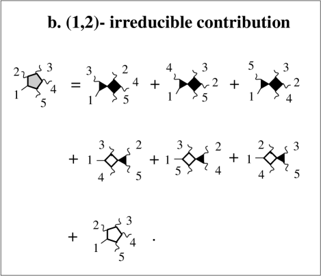
FIG. 14.: Decomposition of the 5th order vertex $D_{4,1}$. Panel a: decomposition of $D_{4,1}$ into one skeleton contribution (first term) and partly reducible 5th order vertex (grey pentagon). Panel b: further decomposition of $D_{4,1}$ into reducible (skeleton) contributions (first three term) and a fully irreducible contribution (empty pentagon).

Examples of reducible (skeleton) contributions to a 5th order vertex are shown in Fig. 15.

In a forthcoming paper in collaboration with V. Belinicher we will show that the skeleton contributions to the nth order vertices have the same rescaling symmetry as the full nth order vertex. This observation means that we can achieve a consistent closure by neglecting the irreducible contributions at any given step of the vertex resummation. It is therefore important to observe that the skeleton contributions to the n’th order vertex are always made of lower order vertices. As shown above, the skeleton contributions to the 4th order vertices consist of two triple vertices and those for the 5th order vertices have contributions of two types. Those with full triple vertices connected by two propagator bridges and one full triple vertex with one irreducible 4th order vertex connected by one propagator bridge. We do not present here the skeleton contributions to 6’th order vertices. There are four types of them: 1) Four black triangles on a line, connected via three propagator bridges, 2) Four black triangles in a star configuration with one central triangle connected via three bridges with three other triangles, 3) Two irreducible 4th order vertices (empty squares) connected by a propagator, and 4) a triple vertex (black triangle) connected via a propagator to a 5th order irreducible vertex.

FIG. 15.: Examples of skeleton contributions to the 5th order vertex $D_{4,1}$ .

- [1] A. S. Monin and A. M. Yaglom. Statistical Fluid Mechanics: Mechanics of Turbulence, volume II. (MIT Press, Cambridge, Mass., 1973).
- [2] K.R. Sreenivasan and R.A. Antonia, Ann. Rev. of Fluid Mech., 29, 435-472 (1997).
- [3] M. Nelkin. Advan. in Phys., 43,143 (1994).
- [4] Uriel Frisch. Turbulence: The Legacy of A.N. Kolmogorov. (Cambridge University Press, Cambridge, 1995).
- [5] R. Benzi, S. Ciliberto, R. Tripiccione, C. Baudet, F. Massaioli and S. Succi, Phys. Rev. E 48, R29, (1993).
- [6] F. Belin, P. Tabeling and H. Willaime, Physica D 93, 52 (1996).
- [7] K.R. Sreenivasan and P. Kailasnath, Phys. Fluids A 5,512 (1993)
- [8] S. Chen and N. Cao, Phys. Rev. E 52, R5757 (1995).
- [9] A.A. Praskovsky, Phys. Fluids A 4,2589 (1992)
- [10] V.S. L’vov, E. Podivilov and I. Procaccia, Phys. Rev. E, 00, 0000 (June 1997).
- [11] V. I. Belinicher and V. S. L’vov, Zh. Eksp. Teor. Fiz. 93, 1269 (1987) [Sov. Phys. JETP, 66:303–313, 1987].
- [12] V.S. L’vov and I. Procaccia, Phys.Rev.Lett.76, 2898 (1996)
- [13] V.S. L’vov and I. Procaccia Nonperturbative, Phys. Rev. E, 00, 0000 (June 1997).
- [14] V.S. L’vov and I. Procaccia, Phys. Rev. E, 52, 3840 (1995); 52, 3858 (1995); 53,3468 (1996).
- [15] V.I. Belinicher, V.S. L’vov and I. Procaccia, Phys. Rev.E, in preparation.
- [16] H.W. Wyld, Ann. Phys. (N.Y.) 14, 143 (1961)
- [17] P,C. Martin, E.D. Siggia and H.A. Rose, Phys. Rev. A, 8, 423 (1973).
- [18] C . De Dominicis, J. Phys. (Paris), 37, C1-247 (1976).
- [19] H. K. Jansen, Z. Phys. B 23, 377 (1976).
- [20] T.C. Halsey, M.H. Jensen, L.P. Kadanoff, I. Procaccia and B.I. Shraiman, Phys.Rev
- [21] R.H. Kraichnan, J. Fluid Mech. 5, 497 (1959)
- [22] R.H. Kraichnan, Phys. Fluids 8,575 (1965).
- [23] V.S. L’vov and V.V. Lebedev, Phys. Rev. E 47, 1794 (1993)
- [24] A. V. Shit’ko, Dokl. An. SSSR, 158, 1058 (1964).