A Geometrical Model for Stagnant Motion
in Hamiltonian Systems with Many Degrees of Freedom

Introduction    In many Hamiltonian systems, $1/f^{\nu}(0<\nu<2)$ power spectra and long time tails have been observed, for instance, in area preserving mappings, [1, 2] a water cluster, [3] and a ferro-magnetic spin system. [4] The $1/f^{\nu}$ spectra imply that relaxation to equilibrium is slow. They are hence important phenomena of Hamiltonian systems with many degrees of freedom. We are interested in understanding the cause of $1/f^{\nu}$ spectra from the structure of phase space and properties of motion.

To describe $1/f^{\nu}$ spectra, Aizawa introduced a geometrical model for area preserving mappings, which are models of Poincaré mappings for Hamiltonian systems with two degrees of freedom. [5, 6] This model assumes exact self-similar hierarchical structure of phase spaces and produces stagnant motion, namely slow relaxation. We therefore understand that stagnant motion arises from self-similar structure of phase space (often referred to ed as “islands around islands” [7]) and motion trapped to KAM tori or Cantori. Meiss et al. have successfully proposed a similar model. [8] A renormalization group approach, [9, 10] which demonstrates similarity between scale transformations in phase space and in time also supports the picture described above. However, the models [5, 7] are based on the two-dimensionality of the phase space and cannot be directly applied to high dimensional systems.

For systems with many (more than two) degrees of freedom, Aizawa et al.  [6] discussed the origin of the $1/f^{\nu}$ spectra based on the Nekhoroshev theorem. Since the argument is based on the Nekhoroshev theorem, the relation between stagnant motion and the hierarchical structure of phase space is not clear.

Moreover, the assumptions on which the models mentioned above are based do not seem to hold for high-dimensional systems. There exist many sorts of fixed points of Poincaré mappings from the fully elliptic type to the fully hyperbolic type, and only the fully elliptic fixed points yield exact self-similarity as area preserving mappings. Since the ratio of fixed points of the fully elliptic type decreases as the system size becomes large, it seems impossible to assume exact self-similarity in the phase space structure for general high-dimensional Hamiltonian systems. It is believed that KAM tori rapidly disappear as the systems size becomes large, and hence the volume of the region where stagnant motion occurs also decreases. On the other hand, since stagnant motion is frequently observed for Hamiltonian systems with many degrees of freedom, we need to establish a model which yields stagnant motion in systems with many degrees of freedom accordingly.

In this paper, we propose a geometrical model which represents hierarchical structure of phase spaces. The model is an extension of Aizawa’s model to many degrees of freedom, and assumes that sticky zones exist around fixed points of Poincaré mappings even if fixed points are not fully elliptic. In other words, in systems with $N$ degrees of freedom, motion is assumed to be trapped for a time around tori of fewer than $N$ dimensions also.

Types of fixed points    We consider Poincaré mappings $F$ and their fixed points instead of Hamiltonian flows and their periodic orbits. We set the number of degrees of freedom to $n$ for Poincaré mappings which have $2N-2$ dimensional Poincaré sections, where $N$ is degrees of freedom of the Hamiltonian dynamics (i.e. $n=N-1$). Note that we construct a model based on fixed points of $F$ hereafter. We can construct the model based on periodic points of $F$ with period-$k$ by using $F^{k}$ instead of $F$.

Local structure around fixed points is built from a combination of the three elementary types: elliptic, hyperbolic and vortex types, for which the eigenvalues of Jacobian of $F$ are $(e^{i\omega},e^{-i\omega})$, $(r,1/r)$ and $(re^{i\omega},re^{-i\omega},e^{i\omega}/r,e^{-i\omega}/r)$ respectively, where both $\omega$ and $r$ are real.  [11] The local structure is constructed as direct products of these three types.

We assume that there is no vortex type structure for simplicity. Generalization including the vortex type will be given in Ref. ?. Then local structure around a fixed point is constructed by elliptic and hyperbolic types of structure, and there are $n+1$ varieties of fixed points: direct products of $n-i$ elliptic type and $i$ hyperbolic ($i=0,1,\cdots,n$). We define the index of a fixed point as $i$. For instance, a fully elliptic fixed point is index-$0$ and a fully hyperbolic is index-$n$.

Geometrical model and master equation    Let us introduce a geometrical model with the following assumptions:
(G-1) Hierarchical structure is constructed by fixed points of Poincaré mappings in phase spaces.
(G-2) Every sort of fixed points has a sticky zone around it, even if it is not fully elliptic.
We calculate volumes of each level of hierarchy and derive a master equation with some assumptions. The number of the level is put in order by volume, and the base level is level-$0$. We assume that the regions of level-$(l+1),(l+2),\cdots$ are in the region of level-$l$. The schematic picture of this model is described in Fig. 1.

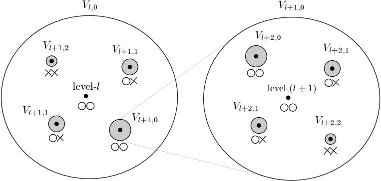
Fig. 1: Schematic picture of the hierarchical structure of phase space. In this picture we assume the system size to be $n=2$. Black points are fixed points. Circle and cross under the fixed points represent elliptic and hyperbolic elementary types, respectively. The double circle, for instance, implies that the structure around the fixed point is a direct product of two elliptic types, namely index-$0$. Let us focus on the left half of this figure. The fixed point at the center, whose index is $0$, belongs to level-$l$, and the other four fixed points belong to level-$(l+1)$. Shaded areas are sticky zones around fixed points of level-$(l+1)$. The sticky zone of the fixed point at the center is the inside of the biggest circle, which includes sticky zones of level-$(l+1)$ fixed points. Level-$(l+2)$ fixed points exist around level-$(l+1)$ fixed points, with a similar situation as on the right half, which is magnification around a fixed point with level-$(l+1)$ and index-$0$.

Let us introduce notation for the quantities which will be used later:

$$N_{l,i} : \mbox{number of fixed points of level-}l,\mbox{ index-}i,$$

$$V_{l,i} : \mbox{volume of a sticky zone around a fixed point of level-}l,\mbox{ index-}i,$$

$$\hat{N}_{l} : \mbox{total number of fixed points of level-}l,$$

$$\hat{V}_{l} : \mbox{total volume of sticky zones of level-}l,$$

$$\rho_{l,i} : \mbox{number of sets of fixed points of level-}(l+1),$$

which surround a fixed point of level-$$l i$$ index-.

Here we have assumed:
(G-3) Fixed points have the same volume $V_{l,i}$ if their level and index are the same.
Note $\hat{V}_{l}>\hat{V}_{l+1}$ for all $l$ because we require that $\hat{V}_{l}$ includes $\hat{V}_{l+1},\hat{V}_{l+2},\cdots$. The meaning of $\rho_{l,i}$ is clarified in the following.

(Fact): A fixed point of level-$l$ and index-$i$ is surrounded by $\rho_{l,i}({}_{n-i}C_{j})$ fixed points of level-$(l+1)$ and index-$(i+j)$, where $j=0,1,\cdots,n-i$, and $\rho_{l,i}$ is a positive integer.

This fact is an extension of the Poincaré-Birkhoff theorem [13] for many degrees of freedom. [14] Using this fact, we write the recursion formula for $N_{l,i}$ as

$$N_{l+1,i}=\sum^{i}_{k=0}\rho_{l,k}N_{l,k}({}_{n-k}C_{i-k}).$$ (1)

The total number $\hat{N}_{l}$ and volume $\hat{V}_{l}$ of the level-$l$ sticky zones are

$$\hat{N}_{l}=\sum^{n}_{i=0}N_{l,i},\qquad\hat{V}_{l}=\sum^{n}_{i=0}N_{l,i}V_{l,i}.$$ (2)

To observe motion among levels we introduce a master equation with the following three assumptions:
(M-1) Systems are ergodic.
(M-2) Transitions from level-$l$ are limited to level-$(l-1)$, $l$ and $(l+1)$.
(M-3) Transitions among levels are Markovian.
From (M-1), the probability being level-$l$ in equilibrium, $P^{\mbox{eq}}_{l}$, is proportional to volume $\hat{V}_{l}$:

$$P^{\mbox{eq}}_{l}\propto\hat{V}_{l}.$$ (3)

We assume detailed balance to fix the transition probability $w_{m,l}\equiv w\{l\to m\}$. Then

$$w_{l,m}P^{\mbox{eq}}_{m}=w_{m,l}P^{\mbox{eq}}_{l}.$$ (4)

From (M-2) and Eqs. (3) and (4), transition probabilities are written as

$$w_{m,l}=\left\{\begin{array}[]{ll}c\hat{V}_{l-1},&(m=l-1)\\ 1-w_{l-1,l}-w_{l+1,l},&(m=l)\\ c\hat{V}_{l+1},&(m=l+1)\\ 0.&(\mbox{otherwise})\end{array}\right.$$ (5)

The factor $c$ is independent of the level, and we set $c=1/(2(\hat{V}_{0}+\hat{V}_{2}))$. By using these transition probabilities, the master equation is written as

$$P_{l}(t+1)=\sum_{m}w_{l,m}P_{m}(t),$$ (6)

where $P_{l}(t)$ is the probability of being on level-$l$ at step $t$.

Results of numerical calculations    We numerically calculated residence time distributions based on our model Eq. (6) and examined if it obeys a power law. The residence time distribution $R(t)$ is the probability that motion extends to levels shallower than level-$l_{\mbox{th}}$ for the first time with initial level being $l_{\mbox{th}}$ at $t=0$. We obtain $R(t)$ from the following transition probabilities and initial condition:

$$w_{m,l_{\mbox{th}}-1}=0\quad(m=l_{\mbox{th}}-1,l_{\mbox{th}},l_{\mbox{th}}+1),\qquad P_{l}(t=0)=\delta_{l,l_{\mbox{th}}}.$$ (7)

Here $\delta_{l,l_{\mbox{th}}}$ is Kronecker’s delta. Then we have

$$R(t)=P_{l_{\mbox{th}}-1}(t).$$ (8)

If $R(t)$ is of a power type rather than an exponential, motion among levels is stagnant.

Parameters which must be given are assumed as follows:

$$\rho_{l,i}=2,\qquad V_{l,i}=b^{-(l+i)},\qquad l_{\mbox{th}}=1,$$

$$N_{0,0}=1\quad\mbox{and}\quad N_{0,i}=0.\quad(i>0)$$

Sticky zones become small as hyperbolic components increase, and this index dependence of $V_{l,i}$ is an essential point of our model. We assumed that the volume of a sticky zone $V_{l,i}$ decays as $b^{-i}$ with respect to the index-$i$ of the fixed point, since local structure near fixed points is constructed by direct products. Other forms of $V_{l,i}$, for instance $V_{l,i}=b^{-l}\tilde{b}^{-i}$ and $V_{l,i}=\exp[-(l+i^{\alpha})\ln b]$, give similar results to $V_{l,i}=b^{-(l+i)}$ with appropriate values of parameters. The form of $V_{l,i}$ determines which index is dominant in $\hat{V}_{l}$.

Fig. 2: Residence time distributions for various values of the scale factor $b$. Here $n=80$. The magnitude of the longitudinal axis is multiplied by $10^{-1},10^{-2}$ and $10^{-3}$ for $b=40,\ 50$ and $60$, respectively.

The residence time distribution $R(t)$ is shown in Fig. 2 for $n=80$ and various values of $b$. When $b$ is small ($b=30,40$) $R(t)$ is of a power type. Namely, we have

$$R(t)\sim t^{-\beta},$$ (9)

where $\beta$ is $3.4$ and $3.1$ for $b=30$ and $b=40$, respectively. Since $R(t)$ is of a power type, stagnant motion occurs among levels. The stagnant motion is also observed when $n=1$, and hence our model Eq. (6) is consistent with models for area preserving mappings mentioned in the Introduction. The values of $\beta$ are also consistent with those obtained in area preserving mappings which are models of physical systems and give $1.5\leq\beta\leq 3$. [1, 2, 15] As far as we know, $\beta$ has not been calculated in Hamiltonian systems with many degrees of freedom. Appearance of oscillating behavior for $b=50$ and $b=60$ is caused by the weakness of effects of the hierarchy, which become weaker as $b$ increases, because large $b$ implies that level-$(l+1)$ is small compared with level-$l$.

Fig. 3: Dependence on the number of degrees of freedom of residence time distributions with fixed $b=30$. The magnitude of the longitudinal axis is multiplied by $10^{-1},\ 10^{-2},\ 10^{-3}$ and $10^{-4}$ for $n=20,\ 40,\ 60$ and $80$, respectively. The distributions are closer to a power type as $n$ increases.

We display the residence time distribution $R(t)$ for various system size $n$ in Fig. 3, where power law behavior of $R(t)$ is clearly seen. Oscillations found for small $n$ gradually decay as $n$ becomes large, and the distributions are close to a power type as $n$ increases. This is an effect of the many degrees of freedom and indicates that fine tuning of parameters is not necessary to observe $1/f^{\nu}$ spectra in systems with many degrees of freedom.

Summary    To understand $1/f^{\nu}$ spectra and long time tails in Hamiltonian systems with many degrees of freedom, we proposed a geometrical model of phase space, which is an extension of Aizawa’s model. We assumed that sticky zones exist around fixed points of Poincarè mappings even if the fixed points are not fully elliptic, and accordingly, exact self-similarity of phase space is not introduced. We derived a master equation from our model, and found that residence time distributions are of a power type. That is, stagnant motion among levels occurs although phase space does not possess exact self-similarity. The power law behavior becomes clearer as the system size increases.

We express our thanks to members of R-lab. of Nagoya University for useful discussions.

References

- [1] C. F. F. Karney, Physica D8 (1983), 360.
- [2] B. V. Chirikov and D. L. Shepelyansky, Physica D13 (1984), 395.
- [3] A. Baba, Y. Hirata, S. Saito and I. Ohmine, J. Chem. Phys. 106 (1997), 3329, and references therein.
- [4] Y. Y. Yamaguchi, Int. J. Bifurcation and Chaos 7 (1997), 839.
- [5] Y. Aizawa, Prog. Theor. Phys. 71 (1984), 1419.
- [6] Y. Aizawa, Y. Kikuchi, T. Harayama, K. Yamamoto, M. Ota and K. Tanaka, Prog. Theor. Phys. Suppl. 98 (1989), 36.
- [7] J. D. Meiss, Phys. Rev. A3 (1986), 2375.
- [8] J. D. Meiss and E. Ott, Physica D20 (1986), 387.
- [9] D. F. Escande, Phys. Rep. 121 (1985), 165.
- [10] T. Hatori and H. Irie, Prog. Theor. Phys. 78 (1987), 249.
- [11] V. I. Arnold and A. Avez, Ergodic problems in classical mechanics (Benjamin-Cummings, Reading, Massachusetts, 1968), Appendix 29.
- [12] Y. Y. Yamaguchi and T. Konishi, In preparation.
- [13] A. J. Lichtenberg and M. A. Lieberman, Regular and Chaotic Dynamics, Second Edition (Springer-Verlag New York, 1992), p.183.
- [14] V. I. Arnold and A. Avez, Ergodic problems in classical mechanics (Benjamin-Cummings, Reading, Massachusetts, 1968), Appendix 33.
- [15] H. Irie, H. Yamaguchi and M. Sato, Physica D54 (1991), 20.