Dynamical Tunneling in Mixed Systems

Abstract

    We study quantum-mechanical tunneling in mixed dynamical systems between symmetry-related phase space tori separated by a chaotic layer. Considering e.g. the annular billiard we decompose tunneling-related energy splittings and shifts into sums over paths in phase space. We show that tunneling transport is dominated by chaos-assisted paths that tunnel into and out of the chaotic layer via the “beach” regions sandwiched between the regular islands and the chaotic sea. Level splittings are shown to fluctuate on two scales as functions of energy or an external parameter: they display a dense sequence of peaks due to resonances with states supported by the chaotic sea, overlaid on top of slow modulations arising from resonances with states supported by the “beaches”. We obtain analytic expressions which enable us to assess the relative importance of tunneling amplitudes into the chaotic sea vs. its internal transport properties. Finally, we average over the statistics of the chaotic region, and derive the asymptotic tail of the splitting distribution function under rather general assumptions concerning the fluctuation properties of chaotic states.

]

I Introduction

A detailed understanding of how the coexistence of classically regular and chaotic phase space areas is reflected in the corresponding quantum dynamics poses one of the challenging problems in the field of “quantum chaos” [2]. Even though semiclassical theories exist for the two limiting cases of fully integrable [3], or fully chaotic classical dynamics [4], the quantum mechanical properties of systems with “mixed” classical dynamics have up to date not been amenable to a semiclassical formulation. The quest for such a theory is importuned by the fact that mixed systems comprise the majority of dynamical systems found in nature.

Out of the wealth of phenomena reported in mixed systems, a particularly interesting one is genuinely quantum-mechanical in nature: tunneling. A situation that has received much attention is the one in which tunneling takes place between distinct, but symmetry-related regular phase space regions separated by a chaotic layer. Interest surged when it was discovered that energy splittings can increase dramatically with chaoticity of the intervening chaotic layer [5, 6, 7]. This was attributed to a suggested mechanism of chaos-assisted tunneling [6, 8, 9] in which tunneling takes place not in a single tunneling transition, but in a multi-step process containing tunneling transitions between regular tori and the chaotic region, as well as chaotic diffusion inside the chaotic sea. Since a large part of the phase space distance is thus traversed via classically allowed transitions, indirect paths can be expected to carry considerably more tunneling flux than direct ones.

Additional evidence was given by the observation that, apart from an overall enhancement, the tunneling splittings vary rapidly over many orders of magnitude as a function of energy, Planck’s constant $\hbar$ or other systemparameters. This was attributed to the occurrence of avoided crossings between regular doublets and chaotic states [6], which made it possible to further establish chaos-assisted tunneling by studying its effect on statistical properties such as the splitting distribution function. Comparison with predictions of appropriate random matrix models showed very good agreement [2, 9, 10]. However, the lack of a semiclassical description of the tunneling processes remained as a gap between the quantum and the classical picture, and — more importantly — the size of the tunneling amplitudes was unknown in the systems under study, which made a direct and quantitative treatment of the phenomenon impossible.

Both of these problems were addressed in an earlier publication by the authors of this work [11] in which a semiclassical analysis of tunneling processes in the annular billiard was performed, and a formula for the contribution of chaos-assisted paths to the energy splitting was derived. Here, we give a detailed account of our findings. Particular emphasis will lie on the description of how the tunneling rate is affected by phase-space structures within the chaotic region, namely the existence of an intermediate “beach” region sandwiched between classically regular islands and the chaotic sea.

The structure of this Paper is as follows. In Section II, we review the basic ideas underlying this work. Also, we introduce the model system under consideration, the annular billiard. In Section III, we introduce the method of our analysis, the scattering approach to the quantization of closed systems, and explicitly construct the “scattering matrix” $S$ for the annular billiard. We then show in Section IV how the scattering matrix approach can, under rather general assumptions, be implemented to the study of tunneling in phase space. We explain how $S$ can be approximated by a five-block matrix model with different blocks representing regular dynamics on either of the islands, beach motion close to each island, and chaotic dynamics in the center of the chaotic sea. We derive formulas for $S$-matrix eigenphase shifts and splittings in terms of paths passing through different combinations of blocks, laying emphasis on the effects arising from the inclusion of the beach blocks. Additionally, we track how tunneling flux spreads in phase space and give a detailed discussion of the interplay of tunneling probabilities into, and transport properties within the chaotic layer. Finally, in Section V we calculate statistical quantities — such as the splitting distribution function and median values for the splitting — by averaging over the properties of the chaotic block. We conclude with a discussion.

II Dynamical Tunneling

A Classical and Quantum Mechanics of Mixed Systems

1 Correspondence of Wavefunctions with Classical Structures

Systems with classically mixed dynamics display both regular and chaotic behavior, depending on the starting conditions of the trajectory considered. The structure of phase space can conveniently be probed by use of a Poincaré surface of section (PSOS) [12], a phase space cut $\Gamma$ giving rise to the Poincaré map

$$(Q,P)_{i}\mapsto(Q,P)_{f}\ ,\quad(Q,P)_{i/f}=(Q(\mathchoice{{\hbox{\boldmath$\displaystyle x_{i/f}$}}}{{\hbox{\boldmath$\textstyle x_{i/f}$}}}{{\hbox{\boldmath$\scriptstyle x_{i/f}$}}}{{\hbox{\boldmath$\scriptscriptstyle x_{i/f}$}}}),P(\mathchoice{{\hbox{\boldmath$\displaystyle x_{i/f}$}}}{{\hbox{\boldmath$\textstyle x_{i/f}$}}}{{\hbox{\boldmath$\scriptstyle x_{i/f}$}}}{{\hbox{\boldmath$\scriptscriptstyle x_{i/f}$}}}))\ ,$$

where $(Q,P)$ is a set of canonically conjugate variables, and $\mathchoice{{\hbox{\boldmath$\displaystyle x$}}}{{\hbox{\boldmath$\textstyle x$}}}{{\hbox{\boldmath$\scriptstyle x$}}}{{\hbox{\boldmath$\scriptscriptstyle x$}}}_{i/f}\in\Gamma$ are connected by the system dynamics. If one starts out with highly localized distributions and plots iterates of the Poincaré cell ${\cal C_{P}}=\{(Q(\mathchoice{{\hbox{\boldmath$\displaystyle x$}}}{{\hbox{\boldmath$\textstyle x$}}}{{\hbox{\boldmath$\scriptstyle x$}}}{{\hbox{\boldmath$\scriptscriptstyle x$}}}),P(\mathchoice{{\hbox{\boldmath$\displaystyle x$}}}{{\hbox{\boldmath$\textstyle x$}}}{{\hbox{\boldmath$\scriptstyle x$}}}{{\hbox{\boldmath$\scriptscriptstyle x$}}})):\mathchoice{{\hbox{\boldmath$\displaystyle x$}}}{{\hbox{\boldmath$\textstyle x$}}}{{\hbox{\boldmath$\scriptstyle x$}}}{{\hbox{\boldmath$\scriptscriptstyle x$}}}\in\Gamma\}$, then chaotic areas show up as areas which quickly become more or less uniformly covered, while regular motion remains confined to lower-dimensional manifolds on ${\cal C_{P}}$. In a mixed system, both types of structures appear, and one arrives at plots of ${\cal C_{P}}$ such as the one presented in Fig. 2 (see below).

In order to associate a system’s quantum eigenstates $\psi$ with classical features — such as chaotic regions or regular tori — one often uses the Wigner transformation [13] of the projector $|\psi\rangle\langle\psi|$. By smoothing over minimal-uncertainty wavepackets one obtains the Husimi distribution [14] that defines a real, non-negative probability density in phase space. We will tacitly invoke the Wigner/Husimi concept in the sequel when referring to the correspondence of quantum states with phase space structures.

Until now, no general theory for the quantization of mixed systems is at hand. However, the understanding has emerged that, in the semiclassical limit, quantum states can unambiguously be classified as “regular” and “chaotic” (for a review, see [6]). Regular states are supported by classical tori obeying EBK quantization rules [3], whereas chaotic states are associated with chaotic phase space regions (or subsets of it [15]). The structure of chaotic states is to date not fully understood and is presently the subject of intensive research. Classification of states as regular and chaotic can become problematic at intermediate energy (or $\hbar$), since EBK-like quantization rules can apply also to states residing on chaotic phase space regions lying in close proximity to the regular island [16, 17, 7]. Loosely speaking, the regularity of classical islands can quantum-mechanically extend into the chaotic sea, and states of an intermediate nature emerge.

2 Effect of Phase Space Symmetries

To discuss the effect of phase space symmetries on the structure of quantum states, we consider a system with a discrete two-fold phase space symmetry ${\cal T}$. We suppose that there are two disjoint phase space objects ${\cal A}_{1}$ and ${\cal A}_{2}$, each of which is invariant under the classical dynamics, mapped onto another by the symmetry operation, ${\cal A}_{2}={\cal T}{\cal A}_{1}$. We also suppose that, in the semiclassical limit, each of the ${\cal A}_{1/2}$ supports a set of states primarily localized on it. Let us, for the sake of definiteness, consider the case when the ${\cal A}_{1/2}$ are EBK-quantized tori. On each of the tori, one can construct quasi-modes $\psi_{r}^{\,(1)}(\mathchoice{{\hbox{\boldmath$\displaystyle q$}}}{{\hbox{\boldmath$\textstyle q$}}}{{\hbox{\boldmath$\scriptstyle q$}}}{{\hbox{\boldmath$\scriptscriptstyle q$}}})$ and $\psi_{r}^{\,(2)}(\mathchoice{{\hbox{\boldmath$\displaystyle q$}}}{{\hbox{\boldmath$\textstyle q$}}}{{\hbox{\boldmath$\scriptstyle q$}}}{{\hbox{\boldmath$\scriptscriptstyle q$}}})=\psi_{r}^{\,(1)}({\cal T}\mathchoice{{\hbox{\boldmath$\displaystyle q$}}}{{\hbox{\boldmath$\textstyle q$}}}{{\hbox{\boldmath$\scriptstyle q$}}}{{\hbox{\boldmath$\scriptscriptstyle q$}}})$ that obey the Schrödinger equation to any order of $\hbar$ [18]. The corresponding EBK energy eigenvalues $E_{r}$ are then degenerate to any order in $\hbar$. However, exact quantum states are constrained to be symmetric or antisymmetric under ${\cal T}$,

$$\psi_{r}^{\,\pm}(\mathchoice{{\hbox{\boldmath$\displaystyle q$}}}{{\hbox{\boldmath$\textstyle q$}}}{{\hbox{\boldmath$\scriptstyle q$}}}{{\hbox{\boldmath$\scriptscriptstyle q$}}})\approx\frac{1}{\sqrt{2}}\left(\psi_{r}^{\,(1)}(\mathchoice{{\hbox{\boldmath$\displaystyle q$}}}{{\hbox{\boldmath$\textstyle q$}}}{{\hbox{\boldmath$\scriptstyle q$}}}{{\hbox{\boldmath$\scriptscriptstyle q$}}})\pm\psi_{r}^{\,(2)}(\mathchoice{{\hbox{\boldmath$\displaystyle q$}}}{{\hbox{\boldmath$\textstyle q$}}}{{\hbox{\boldmath$\scriptstyle q$}}}{{\hbox{\boldmath$\scriptscriptstyle q$}}})\right)\ ,$$ (1)

and the energy degeneracy is lifted by tunneling processes by an amount $\delta E_{r}$, giving rise to tunneling oscillations with period $2\pi\hbar/\delta E_{r}$.

The best-known example of quantum-mechanical tunneling oscillations is the one-dimensional symmetric double quantum well, where the phase space symmetry ${\cal T}(x,p)=(-x,-p)$ connects regular tori in each of the wells (for a careful discussion along the above line of argument, see [9]). In systems of more than two-dimensional phase space, symmetries can give rise to more intricate situations. The tori ${\cal A}_{1}$ and ${\cal A}_{2}$ must not necessarily be separated by an energy barrier in configuration space, but the transition from ${\cal A}_{1}$ to ${\cal A}_{2}$ can also be forbidden by a dynamical law. In this case, there is a dynamical variable other than energy that is conserved by classical dynamics, but violated by quantum dynamics [19, 20]. The case of quantum doublets connected by tunneling processes of this type was first reported by Davis and Heller [21] who also coined the term dynamical tunneling. A particularly clear example of dynamical tunneling will be presented in Section II C in the discussion of the annular billiard. As in the case of energy barrier tunneling, splittings due to dynamical tunneling can be expected to be very small, since classical transport from ${\cal A}_{1}$ to ${\cal A}_{2}$ is forbidden.

Note that the formation of doublets is determined by the phase space topology of the supporting region, not its regularity or chaoticity. The occurrence of doublets has also been observed in situations, in which the localizing mechanism was due to dynamical localization [17, 7, 22] or scarring [23]. Conversely, a phase space structure ${\cal B}={\cal T}{\cal B}$ mapped onto itself supports states that do not form doublets, regardless of its dynamical nature.

B Chaos-Assisted Tunneling

Apart from the possibility of dynamical tunneling, tunneling processes in systems of more than one degree of freedom can have an additional aspect of interest: the appearance of chaos in the region of phase space traversed by the tunneling flux. As an early paradigm of such a system, Lin and Ballentine [5] proposed the periodically driven double well potential, where chaoticity can gradually be introduced by increasing the driving strength. Lin and Ballentine performed a numerical study of tunneling oscillations between states associated with regular tori corresponding to classical motion confined to either bottom of the well. They observed that, as the separating phase space layer grows more chaotic with increasing driving strength, tunneling rates are enhanced by orders of magnitude over the rate in the undriven system (the integrable 1-$d$ double well). In a later study of the same system, Utermann et al. [7] established that the tunneling rate of a wave packet initially localized on one regular island is determined not by the wave packet’s overlap with the other island, but by its overlap with the chaotic sea, pointing at a role for classically chaotic diffusion as a mediator of quantum tunneling flux.

In a parallel and simultaneous line, Bohigas, Tomsovic and Ullmo advocated the interpretation that the enhancement of tunneling was a case of resonant tunneling due to the occurrence of avoided crossings of the tunneling doublet’s eigenenergies with the eigenenergy of a state residing on the intervening phase space layer [6]. For obvious reasons, the phenomenon was named chaos-assisted tunneling. The interpretation of tunneling enhancement in terms of a three-level process was derived from the observation that splittings of regular doublets are rapidly fluctuating quantities as functions of parameters such as energy, Planck’s constant $\hbar$, or other model parameters — much in contrast to the smooth, at most oscillatory, dependence of tunneling rates on $\hbar$, say, in the case of energy barrier tunneling [24].

Since a semiclassical description of tunneling matrix elements was lacking, Bohigas and coworkers focussed on the statistical fingerprints of chaos-assisted tunneling, with emphasis on the consequences of resonance denominators on the splitting distribution. To this end, the interaction of regular doublets with chaotic states was formulated in terms of a block matrix model [6], in which properties of states residing on the chaotic sea were approximated by use of random matrix theory [25]. This model was subsequently refined by Tomsovic and Ullmo [9] to take into account the effect of additional time scales in the chaotic dynamics that can appear when residual phase space structures, such as cantori, are present in the chaotic sea acting as imperfect transport barriers. Predictions made using these block-matrix models showed good agreement with numerically calculated splitting distributions. Along these lines, Ullmo and Leyvraz [10] were also able to derive analytic expressions for the splitting distributions in the case of structure-less chaotic dynamics, as well as for a structured chaotic sea. Again, theoretical predictions showed good agreement with exact numerical data.

C The Annular Billiard

We now introduce the specific system under consideration in this work, the annular billiard. It was proposed by Bohigas et al. [8] and consists of the area trapped between two non-concentric circles of radii $R$ and $a<R$ centered at $(x,y)$ coordinates $O\equiv(0,0)$ and $O^{\prime}\equiv(-\delta,0)$, respectively. We consider the case of $\delta<a$ and set $R=1$, unless otherwise stated. Note that the billiard is symmetric under reflections at the $x$-axis.

FIG. 1.: Parameterization of classical trajectories. Note that coordinates $(\gamma,L)$ are not the Birkhoff coordinates $(\varphi,L)$ usually employed in billiards. The two coordinate sets are related by $\varphi=\gamma+\alpha-\pi$, where $\alpha=\arcsin(L/R)$.

1 Classical Dynamics

Classical motion in a billiard is given as free flight between specular reflections at the boundaries. We select the PSOS $\Gamma$ as a circle of radius $r$ concentric with the outer circle and choose $r$ to be infinitesimally smaller than one. Upon in-bound passage through $\Gamma$ — or, equivalently, after reflection from the outer circle — we record the trajectory’s coordinates $(\gamma,L)$, where $\gamma$ denotes the angle of the velocity vector with the $x$-axis and $L=\sin\alpha$ is the classical impact parameter with respect to $O$ (see Fig. 1). $(\gamma,L)$ are canonically conjugate with respect to the reduced action [20], and the Poincaré cell is given by ${\cal C_{P}}=[0,2\pi]\times]-1,1[$. The billiard’s mirror symmetry $y\mapsto-y$ translates into an invariance of ${\cal C_{P}}$ under the mapping $(\gamma,L)\mapsto(2\pi-\gamma,-L)$.

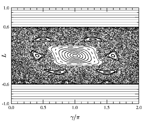
FIG. 2.: Poincaré plot of classical motion in the annular billiard at $a=0.4$ and $\delta=0.2$.

In Fig. 2 we present a Poincaré plot of ${\cal C_{P}}$ at parameter values $a=0.4$ and $\delta=0.2$. Rays of $|L|>a+\delta$ do not hit the inner circle, but forever encircle the inner disc at constant $L$ filling horizontal strips (or subsets of horizontal strips) in the Poincaré plot. Each of these whispering gallery (WG) tori, specified by its impact parameter $L$, is associated with a partner torus $-L$ by the mirror symmetry. These WG tori will be the tunneling tori under consideration in this work.

Rays of intermediate impact parameter $|L|<a+\delta$ will eventually hit the inner circle, and since angular momentum is then not preserved, motion is no longer integrable. This can give rise to the whole range of phenomena associated with non-integrable systems of mixed phase space: regular islands and island chains, chaotic regions, partial transport barriers (cantori) and the like. The structure of the phase space layer $|L|<a+\delta$ is primarily organized by two fixed points of the Poincaré map: (i) an unstable fixed point at $(\gamma,L)=(0,0)$ and its stable and unstable manifolds, along which a chaotic region spreads out, and (ii) a stable orbit $(\gamma,L)=(\pi,0)$ at the center of a regular island of “libration” trajectories. The fixed points correspond to rays along the symmetry axis on the left hand side and on the right hand side of the inner circle, respectively.

It will turn out to be of great importance that there is a region of chaotic, but relatively stable motion surrounding each regular island. In the strip of $|L|\lesssim a+\delta$ this stability is easy to understand, as trajectories typically encircle the inner disc many times until a hit occurs, and at each hit the change in impact parameter is small. The “stickiness” of this beach region is increased by the presence of regular island chains and of cantori that are the remains of broken WG tori.

2 Quantum Mechanics

Quantum mechanics of the annular billiard with Dirichlet boundary conditions is given by the Helmholtz equation

$\displaystyle(\Delta+k^{2})\,\psi(\mathchoice{{\hbox{\boldmath$\displaystyle q$}}}{{\hbox{\boldmath$\textstyle q$}}}{{\hbox{\boldmath$\scriptstyle q$}}}{{\hbox{\boldmath$\scriptscriptstyle q$}}})=0$

and the requirement of vanishing wavefunction on the two circles. The wave number $k$ is related to energy by $E=\hbar^{2}k^{2}/2m$. (We note that there exists an analogy between quantum billiards and quasi-two-dimensional microwave resonator which has proven instrumental in many experimental realizations of billiard systems [26].)

We give here only a qualitative picture of the quantum states, deferring a full solution to Section III B. It is most appropriate to decompose the wavefunction into angular momentum components by writing

$$\psi(r,\varphi)\!=\!\sum_{n=-\infty}^{\infty}\!i\,^{n}\left[\alpha_{n}\mathop{\rm H{}}^{\text{\,(2)}}\nolimits_{n}(kr)+\beta_{n}\mathop{\rm H{}}^{\,(1)}\nolimits_{n}(kr)\right]\text{e}^{in\varphi}\ ,$$ (2)

where $(r,\varphi)$ are polar coordinates with respect to $O$, and $\mathop{\rm H{}}^{\,(1,2)}\nolimits_{n}(x)$ denote Hankel functions of the first and second kind, respectively, of order $n$. We recall that angular momentum quantum numbers $n$ are in the semiclassical limit related to classical impact parameters $L=n/k$.

To understand the nature of quantum states supported by the annular billiard, it is instructive to first consider the concentric billiard and then to “turn on” the eccentricity $\delta$. If $\delta=0$, then angular momentum is conserved, and states are paired in energetically degenerate doublets composed of angular momentum components $n$ and $-n$. In the eccentric system ($\delta\neq 0$), the degeneracy is lifted by the breaking of rotational invariance. However, angular momentum doublets are affected to different degrees — depending on the size of $n$ relative to $k(a+\delta)$. The symmetry breaking has large effect on doublets of small angular momentum $|n|<k(a+\delta)$ corresponding to classical motion that can hit the inner circle. For low-$n$ doublets, the doublet pairing disappears quickly with increasing $\delta$ and “chaotic” eigenstates appear that spread out in angular momentum components roughly between $-k(a+\delta)$ and $k(a+\delta)$. High-angular momentum doublets with $|n|>k(a+\delta)$ are affected only little by the symmetry breaking. The doublet-pairing persists, and energy degeneracy is only slightly lifted. States are primarily composed of symmetric and antisymmetric combinations of $n$ and $-n$ angular momentum components,

$$\mid\mathchoice{{\hbox{\boldmath$\displaystyle\alpha$}}}{{\hbox{\boldmath$\textstyle\alpha$}}}{{\hbox{\boldmath$\scriptstyle\alpha$}}}{{\hbox{\boldmath$\scriptscriptstyle\alpha$}}}^{\,(\pm)}\>\rangle\approx\frac{1}{\sqrt{2}}\big{(}\mid n\>\rangle\pm\mid-n\>\rangle\big{)}\ .$$ (3)

Note that each of the quasi-modes $|\pm n\rangle$ corresponds to classical motion on the WG torus $\pm L$.

We present plots of a “regular” doublet quantized at $k\approx 55$ and a “chaotic” state at $k\approx 60$ in Fig. 3 and compare them to classical trajectories with starting conditions in the chaotic sea and on WG tori, respectively. The correspondence between quantum states and the nature of classical dynamics is clearly visible.

FIG. 3.: Comparison of classical dynamics and quantum states of the annular billiard. (a–c) Classical motion: (a,c) regular trajectories of $\pm L$, $|L|>a+\delta$, (b) chaotic trajectory of $|L|<a+\delta$. (a–c) Eigenmodes: (a,c) doublet of “regular” eigenstates at $k\approx 54.434$, and (b) “chaotic” eigenstate at $k\approx 60.252$.

3 Tunneling Between Whispering Gallery Tori

Let us discuss the high-angular momentum doublets in more detail. As explained above, the energy splitting $\delta E_{n}$ between $|\mathchoice{{\hbox{\boldmath$\displaystyle\alpha$}}}{{\hbox{\boldmath$\textstyle\alpha$}}}{{\hbox{\boldmath$\scriptstyle\alpha$}}}{{\hbox{\boldmath$\scriptscriptstyle\alpha$}}}^{\,(+)}\rangle$ and $|\mathchoice{{\hbox{\boldmath$\displaystyle\alpha$}}}{{\hbox{\boldmath$\textstyle\alpha$}}}{{\hbox{\boldmath$\scriptstyle\alpha$}}}{{\hbox{\boldmath$\scriptscriptstyle\alpha$}}}^{\,(-)}\rangle$ gives rise to tunneling oscillations between quasi-modes $|\pm n\rangle$ associated with WG tori $\pm L=\pm n/k$ $(L>a+\delta)$. A quantum particle prepared in state $|n\rangle$ will therefore change its sense of rotation from counter-clockwise to clockwise and back to counter-clockwise with period $2\pi\hbar/\delta E_{n}$. Note that this tunneling process serves as a particularly clear example of dynamical tunneling. It occurs in phase space rather than configuration space, as the corresponding tori are identical in configuration space. Also, the tunneling process does not pass under a potential barrier in configuration space. In fact, energy does not play any role in the tunneling, as energy is related only to the absolute value of the momentum vector and not to its direction. Rather, the tunneling process violates the dynamical law of classical angular momentum conservation for rays of large impact parameter.

The concept of chaos-assisted tunneling can be nicely visualized for the case of tunneling between WG modes in the annular billiard. In fact, the annular billiard was proposed as a paradigm for chaos-assisted tunneling in Ref. [8]. In chaos-assisted processes, tunneling tori $\pm L$ are connected not by direct transitions between $n\mapsto-n$, but by multi-step transitions $n\mapsto\ell\ldots-\ell^{\prime}\mapsto-n$. A particle tunnels from $n$ to some $\ell\lesssim k(a+\delta)$, traverses the chaotic phase space layer by classically allowed transitions to reach the opposite side of the chaotic sea $-\ell^{\prime}\gtrsim-k(a+\delta)$, and finally tunnels from there to $-n$. To establish this notion, Bohigas et al. [8] checked the behavior of splittings as the eccentricity is changed to make the intervening phase space layer more chaotic. In a numerical study, they compared the splittings of regular doublets with the rate of classical transport across the chaotic layer. The findings showed that the splittings increase dramatically over many orders of magnitude as chaotic transport becomes quicker.

However, without a quantitative — possibly semiclassical — theory, it is impossible to separately analyze the importance of tunneling amplitudes and transport properties of the intervening chaotic layer. Usually, the parameter governing symmetry breaking in a mixed system changes both tunneling amplitudes from/into the regular torus and chaoticity in the intermediate layer. In order to separate the relative importance of these effects, a quantitative understanding of the tunneling processes must be obtained. Such a quantitative description of chaos-assisted tunneling was given in Ref. [11] and will be developed in full detail in the sequel.

III Quantization by Scattering

A General Description of the Method

In this work, we will employ an scattering approach to quantization [27, 28] which, in essence, is constructed as the quantum-mechanical analogue of the classical Poincaré surface of section method. For the sake of self-containedness, we give a brief review of the scattering method.

Let us consider the case of a billiard ${\cal G}$ and introduce a Poincaré cut $\Gamma$ in configuration space, thereby dividing ${\cal G}$ into two parts, ${\cal G}_{+}$ and ${\cal G}_{-}$. We suppose that $\Gamma$ can be chosen along a coordinate axis (the $q_{2}$-axis, say) and that the wave problem is separable on an infinitesimal strip around $\Gamma$. At a given energy, one chooses a complete set of functions $\phi_{n}^{(2)}(q_{2})$ along $\Gamma$ and writes the wavefunction on an infinitesimal strip around $\Gamma$ as

$$\psi(\mathchoice{{\hbox{\boldmath$\displaystyle q$}}}{{\hbox{\boldmath$\textstyle q$}}}{{\hbox{\boldmath$\scriptstyle q$}}}{{\hbox{\boldmath$\scriptscriptstyle q$}}})=\sum_{n}\left(\alpha_{n}\phi_{n}^{(1,-)}(q_{1})+\beta_{n}\phi_{n}^{(1,+)}(q_{1})\right)\phi^{(2)}_{n}(q_{2})\ .$$ (4)

$\phi_{n}^{(1,+)}$ and $\phi_{n}^{(1,-)}$ are functions that, in the semiclassical limit, correspond to waves traversing $\Gamma$ in positive and negative $q_{1}$-direction, respectively. We assume that the set $\phi_{n}^{(2)}(q_{2})$ is chosen such that quantum numbers $n$ correspond to values $k^{(2)}_{n}$ of longitudinal wave number. Then, $k_{n}^{(2)}$ and transverse wave numbers $k_{n}^{(1)}$ are related by $E_{n}=\hbar^{2}[(k_{n}^{(1)})^{2}+(k_{n}^{(2)})^{2}]/2m$. Note that orthogonality of the modes on $\Gamma$ is ensured by the choice of the $\phi_{n}^{(2)}$. Each of the domains ${\cal G}_{\pm}$ constitutes a scattering system that scatters waves $\phi_{n}^{(1,+)}\,\phi_{n}^{(2)}$ into waves $\phi_{n}^{(1,-)}\,\phi_{n}^{(2)}$ and vice versa. Associated with these scattering systems ${\cal G}_{\pm}$ are scattering matrices $S_{\pm}(E)$ that relate the coefficient vectors

$$\mathchoice{{\hbox{\boldmath$\displaystyle\beta$}}}{{\hbox{\boldmath$\textstyle\beta$}}}{{\hbox{\boldmath$\scriptstyle\beta$}}}{{\hbox{\boldmath$\scriptscriptstyle\beta$}}}\>=\>S_{-}(E)\,\mathchoice{{\hbox{\boldmath$\displaystyle\alpha$}}}{{\hbox{\boldmath$\textstyle\alpha$}}}{{\hbox{\boldmath$\scriptstyle\alpha$}}}{{\hbox{\boldmath$\scriptscriptstyle\alpha$}}}\qquad\text{ and }\qquad\mathchoice{{\hbox{\boldmath$\displaystyle\alpha$}}}{{\hbox{\boldmath$\textstyle\alpha$}}}{{\hbox{\boldmath$\scriptstyle\alpha$}}}{{\hbox{\boldmath$\scriptscriptstyle\alpha$}}}\>=\>S_{+}(E)\,\mathchoice{{\hbox{\boldmath$\displaystyle\beta$}}}{{\hbox{\boldmath$\textstyle\beta$}}}{{\hbox{\boldmath$\scriptstyle\beta$}}}{{\hbox{\boldmath$\scriptscriptstyle\beta$}}}\ .$$ (5)

The quantization condition is equivalent to the requirement of single-valuedness of the wave function on $\Gamma$, and so to the equivalence of the two scattering conditions. The system supports an eigenstate whenever the product matrix

$\displaystyle S(E)\equiv S_{-}(E)\,S_{+}(E)$

has an eigenvalue of unity, hence the quantization condition reads

$$\det(S(E)-1)=0\ .$$ (6)

At a quantized energy, the wave function can be reconstructed from the corresponding eigenvector $\textstyle\alpha$ of $S$ via Eqs. (4,5). In principle, $S$ is an infinite-dimensional matrix. However, in many cases of interest one can choose the $\phi_{n}^{(1,+)}\,\phi_{n}^{(2)}$ so that in the region of classically allowed motion, the contribution $|\phi_{n}^{(1,\pm)}(q_{1})|$ is exponentially small for all but a finite number of indices (the so-called “open channels”). This allows the truncation of $S$ to finite dimension, say $|n|\leq\Lambda$, with an error that is exponentially small. Both scattering matrices $S_{\pm}$ can be constructed in a representation such that they are unitary in the space of open modes and, if the system is time-reversal invariant, symmetric. $S$ on the other hand is unitary, but not necessarily symmetric. In spite of this, we will in this paper also refer to $S$ as a scattering matrix.

It is clear by construction that $S$ is the quantum-mechanical analogue of the Poincaré mapping [29]. Its $N$-th iterate $S^{N}$ constitutes a time-domain-like propagator. Note that the iteration count $N$ of the Poincaré map does not correspond to a stroboscopic discretization of time, but rather to a fictitious discrete time, since generally the time elapsed between passages of $\Gamma$ can vary. If, however, we select our surface of section properly, then return times will not vary by too much, and $S$ will not be too different from the genuine time-domain propagator.

B Scattering Matrix of the Annular Billiard

It is fairly straightforward to implement the scattering approach to the case of the annular billiard. As discussed in Section II C, we choose $\Gamma$ as a circle of radius $r$, where $a+\delta<r\lesssim 1$. Since classical impact parameter is conserved by motion on the WG tori, we choose $q_{2}=\varphi$ and $\phi_{n}^{\,(2)}=\exp(in\varphi)$ on $\Gamma$. Waves traversing $\Gamma$ are given by outgoing and ingoing cylinder waves $\phi_{n}^{\,(1,+)}=i^{n}\mathop{\rm H{}}^{\,(1)}\nolimits_{n}(kr)$, $\phi_{n}^{\,(1,-)}=i^{n}\mathop{\rm H{}}^{\,(2)}\nolimits_{n}(kr)$, and we obtain the decomposition in Eq. (2),

$$\psi(r,\varphi)\!=\!\sum_{n=-\infty}^{\infty}i^{n}\left[\alpha_{n}\mathop{\rm H{}}^{\text{\,(2)}}\nolimits_{n}(kr)+\beta_{n}\mathop{\rm H{}}^{\,(1)}\nolimits_{n}(kr)\right]\text{e}^{in\varphi}\ .$$ (7)

In the present example, outgoing waves are scattered to ingoing waves by the interior of the outer circle — giving rise to the scattering condition $\mathchoice{{\hbox{\boldmath$\displaystyle\alpha$}}}{{\hbox{\boldmath$\textstyle\alpha$}}}{{\hbox{\boldmath$\scriptstyle\alpha$}}}{{\hbox{\boldmath$\scriptscriptstyle\alpha$}}}=S^{\,\text{(O)}}(k)\,\mathchoice{{\hbox{\boldmath$\displaystyle\beta$}}}{{\hbox{\boldmath$\textstyle\beta$}}}{{\hbox{\boldmath$\scriptstyle\beta$}}}{{\hbox{\boldmath$\scriptscriptstyle\beta$}}}\>$ — and ingoing waves are reflected off the exterior of the inner circle, which leads to the relation $\mathchoice{{\hbox{\boldmath$\displaystyle\beta$}}}{{\hbox{\boldmath$\textstyle\beta$}}}{{\hbox{\boldmath$\scriptstyle\beta$}}}{{\hbox{\boldmath$\scriptscriptstyle\beta$}}}=S^{\,\text{(I)}}(k)\,\mathchoice{{\hbox{\boldmath$\displaystyle\alpha$}}}{{\hbox{\boldmath$\textstyle\alpha$}}}{{\hbox{\boldmath$\scriptstyle\alpha$}}}{{\hbox{\boldmath$\scriptscriptstyle\alpha$}}}\>$. In order to derive the explicit formulas for $S^{\,\text{(O)}}$ and $S^{\,\text{(I)}}$, we note that the Dirichlet boundary condition $\psi(R,\varphi)=0$ on the outer circle leads to

$$S^{\,\text{(O)}}_{n,m}(k)=-\frac{\mathop{\rm H{}}^{\,(1)}\nolimits_{n}(kR)}{\mathop{\rm H{}}^{\,(2)}\nolimits_{n}(kR)}\>\delta_{n,m}\ .$$ (8)

$S^{\,\text{(O)}}(k)$ is diagonal, in accordance with angular momentum conservation in scattering events off the outer circle.

$S^{\,\text{(I)}}(k)$ is derived by performing a coordinate change to the primed coordinates defined with respect to $O^{\prime}=(\delta,0)$. In this representation the scattering matrix is $S^{\,\prime\,\text{(I)}}(k)=-\mathop{\rm H{}}^{\,(2)}\nolimits_{n}(ka)/\mathop{\rm H{}}^{\,(1)}\nolimits_{n}(ka)\,\delta_{n,m}$. Transformation back to unprimed coordinates is done by the addition theorem for Bessel functions (see e.g. [30])

$\displaystyle\mathop{\rm H{}}^{\,(1,2)}\nolimits_{n}(kr)\,\mbox{\rm e}\,^{in\varphi}=\sum_{\ell=-\infty}^{\infty}\mbox{\rm J}_{n-\ell}(k\delta)\,\mathop{\rm H{}}^{\,(1,2)}\nolimits_{\ell}(kr^{\prime})\,\mbox{\rm e}\,^{i\ell\varphi^{\prime}}$

for $\delta<a=r^{\prime}$. $\mbox{\rm J}_{n}(x)=(\mathop{\rm H{}}^{\,(1)}\nolimits_{n}(x)+\mathop{\rm H{}}^{\,(2)}\nolimits_{n}(x))/2$ denotes the Bessel function of order $n$. We arrive at

$$S^{\,\text{(I)}}_{n,m}(k)=-i^{(n-m)}\sum_{\ell=-\infty}^{\infty}\mathop{\rm J{}}\nolimits_{n-\ell}(k\delta)\,\mathop{\rm J{}}\nolimits_{m-\ell}(k\delta)\>\frac{\mathop{\rm H{}}^{\text{\,(2)}}\nolimits_{\ell}(ka)}{\mathop{\rm H{}}^{\,(1)}\nolimits_{\ell}(ka)}\;.$$

Time-reversal invariance imposes the symmetry$S^{\,\text{(I)}}_{m,n}(k)=(-)^{(n-m)}\,S^{\,\text{(I)}}_{n,m}(k)$ on $S^{\,\text{(I)}}(k)$ and by virtue of the mirror symmetry $S^{\,\text{(I)}}_{-n,-m}(k)=S^{\,\text{(I)}}_{n,m}(k)$. (Note that the formula given for $S^{\,\text{(I)}}(k)$ differs by the factor $i\,^{(n-m)}$ from a formula given earlier by us [11] and consequently, also the symmetries are different. This is due to a slightly different choice of basis in (7).) The full $S$-matrix is then given as

$$S_{n,m}(k)=$$ (9)

$$i\,^{(n-m)}\frac{\mathop{\rm H{}}^{\,(1)}\nolimits_{n}(kR)}{\mathop{\rm H{}}^{\,(2)}\nolimits_{n}(kR)}\,\sum_{\ell=-\infty}^{\infty}\mathop{\rm J{}}\nolimits_{n-\ell}(k\delta)\,\mathop{\rm J{}}\nolimits_{m-\ell}(k\delta)\>\frac{\mathop{\rm H{}}^{\text{\,(2)}}\nolimits_{\ell}(ka)}{\mathop{\rm H{}}^{\,(1)}\nolimits_{\ell}(ka)}\;.$$ (10)

     

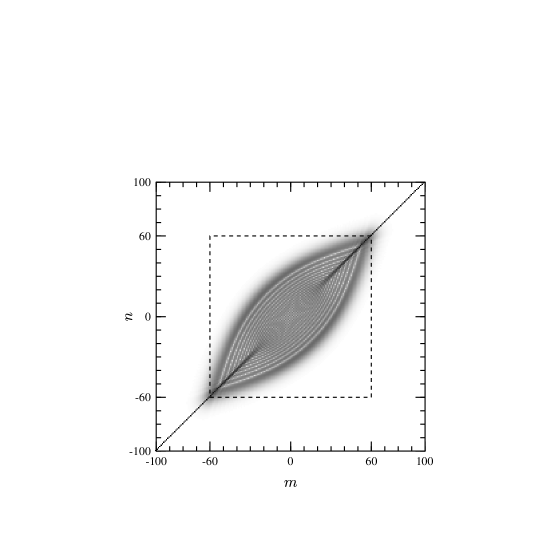
FIG. 4.: Grayscale plot of the quantum $S$-matrix $|S{{}_{n},m}|$ (arbitrary gray scale). The dashed line indicates the region of classical angular momentum mixing $|n|<k(a+\delta)$.

Using the relation $\mathop{\rm H{}}^{\,(1,2)}\nolimits_{-n}(x)=(-)^{n}\mathop{\rm H{}}^{\,(1,2)}\nolimits_{n}(x)$ for integer $n$, one verifies that the spatial symmetry of the annular billiard translates into the $S$-matrix symmetry

$$S_{-n,-m}\>=\>S_{n,m}\ .$$ (11)

For eigenvectors $\mathchoice{{\hbox{\boldmath$\displaystyle\alpha$}}}{{\hbox{\boldmath$\textstyle\alpha$}}}{{\hbox{\boldmath$\scriptstyle\alpha$}}}{{\hbox{\boldmath$\scriptscriptstyle\alpha$}}}^{(j)}$ of $S$,

$$\alpha_{-n}^{(j)}={\sigma_{j}}\,\alpha_{n}^{(j)}\ ,$$ (12)

where $\sigma_{j}\in\{\pm 1\}$. Whenever the system supports an eigenstate, $\sigma_{j}$ determines the symmetry of the corresponding wave function with respect to the $x$-axis.

In Fig. 4, we show a grayscale plot of $|S_{n,m}|$ as a function of ingoing and outgoing angular momentum for the parameter values $a=0.4$, $\delta=0.2$, $k=100$. The overall structure of $S$ is governed by classically allowed transitions: it is mainly diagonal in the region of high angular momentum $|n|,|m|>k(a+\delta)$, whereas the inner block reflects the dynamics given by the classical deflection function. Here, the main amplitude is delimited by two ridges that correspond to classical rainbow scattering.

The tunneling amplitudes relevant to the WG splitting are contained in $S$ as non-diagonal entries $S_{n,m}$ with $n>k(a+\delta)$. Fig. 5 depicts $|S_{n,m}|$ for the above parameter values and $n=70$ (at $k(a+\delta)=60$).

FIG. 5.: Absolute values of tunneling matrix elements $|S_{n,m}|$ for $n=70$ and $m=-100,\ldots,100$ (logarithmic scale). Inset: first quadrant of $S$, showing the tunneling ridges. (Taken from Ref. [11].)

The tunneling amplitudes are largest ($\sim 10^{-4}$) around $m=63$ and fall off faster than exponentially away from this maximum. As can be seen in the inset of Fig. 5, the line of maximal tunneling amplitudes continues the line of rainbow ridges into the regime of classically forbidden transitions. Close to these tunneling ridges, and in the direction away from the diagonal, one can observe oscillations in $|S_{n,m}|$ that resemble the Airy oscillations well-known in diffraction theory [31]. It is interesting to note that the behavior of the tunneling probabilities is not a monotonous function of $|n-m|$, that is, of the phase space distance traversed. A mere distance in phase space can therefore not serve to estimate the behavior of tunneling probabilities.

We finally mention that the tunneling transitions considered here can be given a semi-classical interpretation in terms of complex rays that interact with the analytical continuation of the inner circle to complex configuration space [11, 32, 33]. These rays can either scatter off the inner complex circle by a generalization of specular reflection, or they can creep along a complexified inner circle (of complex radius determined by the poles of the internal scattering matrix) by a mechanism similar to that proposed by Franz [34] and Keller [35]. Every tunneling pair $n_{i},n_{f}$ is connected by at least one complex reflection trajectory with real initial (final) impact parameter $L_{i}=n_{i}/k$ $(L_{f}=n_{f}/k)$ and complex initial (final) angle $\gamma_{i}$ $(\gamma_{f})$. Complex reflection and creeping trajectories give rise to contributions to the tunneling matrix elements that scale with $k$ like

$$S_{\text{reflection}} \sim k^{-1}\>\exp\Big{(}-kA_{\text{ref}}(i,f)\>\Big{)}\ ,$$ (13)

$$S_{\text{creeping}} \sim k^{-2/3}\>\exp\Big{(}-kA_{\text{cr}}(i,f)+k^{1/3}B_{\text{cr}}(i,f)\>\Big{)}\ ,$$ (14)

respectively, where $A_{\text{ref}}$, $A_{\text{cr}}$ and $B_{\text{cr}}$ are classical properties of the associated trajectories that are independent of $k$. The relative importance of the two contributions depends on $k$, the billiard geometry, and the initial and final angular momenta considered. At the present parameter values, the contribution due to reflected rays usually dominates the one arising from creeping rays.

The semiclassical picture provides an intuitive explanation to the tunneling ridges mentioned above: they can be identified as combinations $n,m$ where one of the angles $\gamma_{i},\gamma_{f}$ is closest to reality. Also, the nearby oscillations can be understood as arising from a coalescence of two reflection saddle points.

IV Treatment of Chaos-Assisted Tunneling

A Implementation of the Scattering Approach

We now discuss how the scattering approach can be implemented to the treatment of chaos-assisted tunneling. Let us suppose that the system under consideration has a phase space symmetry of type $(q_{2},p_{2})\mapsto(-q_{2},-p_{2})$, and that the $q_{2}$-axis can be chosen as a PSOS $\Gamma$. We assume that the wave problem is locally separable around $\Gamma$, which renders the problem tractable by the scattering approach. Let us now pick two classical objects ${\cal A}_{1}$ and ${\cal A}_{2}={\cal T}{\cal A}_{1}$ and consider quasi-modes $\psi_{r}^{\,(1/2)}(\mathchoice{{\hbox{\boldmath$\displaystyle q$}}}{{\hbox{\boldmath$\textstyle q$}}}{{\hbox{\boldmath$\scriptstyle q$}}}{{\hbox{\boldmath$\scriptscriptstyle q$}}})$ supported by ${\cal A}_{1/2}$, as discussed in Section II. We assume that motion on ${\cal A}_{1}$ and ${\cal A}_{2}$ corresponds to conservation of $p_{2}$ and $-p_{2}$, respectively, and that $\pm p_{2}$ is semiclassically related to the quantum number $\pm n$. (Note that in a general system, the choice of the PSOS $\Gamma$ and a proper basis for the scattering matrix can be a very difficult task. In this Paper, we will not deal with the problem of solving a general scattering problem — except for the annular billiard — and assume the scattering matrix $S_{n,m}$ to be known.) By symmetry $p_{2}\mapsto-p_{2}$, we find that $S_{n,n}=S_{-n,-n}$, and by virtue of the classical conservation of $p_{2}$, $S_{n,n}$ is almost unimodular. The deviation of $|S_{n,n}|$ from unity will be due to classically forbidden (i.e. tunneling) transitions, and so is expected to be small.

Let the quantization energies of the doublet be denoted by $E_{n}^{\pm}$, and let $|\mathchoice{{\hbox{\boldmath$\displaystyle\alpha$}}}{{\hbox{\boldmath$\textstyle\alpha$}}}{{\hbox{\boldmath$\scriptstyle\alpha$}}}{{\hbox{\boldmath$\scriptscriptstyle\alpha$}}}^{\pm}(E_{n}^{\pm})\rangle$ be the eigenvectors corresponding to the two quantum states. We now make the approximation that the properties of these two vectors are, to good precision, given by the eigenvector doublet $|\mathchoice{{\hbox{\boldmath$\displaystyle\alpha$}}}{{\hbox{\boldmath$\textstyle\alpha$}}}{{\hbox{\boldmath$\scriptstyle\alpha$}}}{{\hbox{\boldmath$\scriptscriptstyle\alpha$}}}^{\pm}(E)\rangle$ at one fixed energy $E$ lying between $E_{n}^{+}$ and $E_{n}^{-}$. The corresponding (generally non-zero) eigenphases be denoted by $\theta_{n}^{\pm}(E)$.

Dropping the energy variable $E$, we decompose the eigenphases $\theta_{n}^{\pm}$ in the form

$$\theta_{n}^{\pm}\>\equiv\>\theta_{n}^{\,(0)}+\Delta\theta_{n}^{\,(R)}+i\Delta\theta_{n}^{\,(I)}\pm\frac{1}{2}\,\delta\theta_{n}\ ,$$ (15)

where $\Delta\theta_{n}^{\,(R,I)}$ are taken to be real, and $\theta_{n}^{\,(0)}=-i\log S_{n,n}$. The quantities $\Delta\theta_{n}=\Delta\theta_{n}^{\,(R)}+i\Delta\theta_{n}^{\,(I)}$ and $\delta\theta_{n}$ can be interpreted as the shift and the splitting, respectively, of the exact eigenphases due to tunneling processes. These eigenphase quantities are trivially related to the energy shift and splitting, as will be explained below, and it is therefore sufficient to calculate $\Delta\theta_{n}$ and $\delta\theta_{n}$. Note that the $\theta_{n}^{\pm}$ are real by unitarity of $S$, and therefore also $\theta_{n}^{\,(0)}+\Delta\theta_{n}$ and $\delta\theta_{n}$ are real quantities. We also note that

$$\left[S^{N}\right]_{\pm,\pm} \equiv \langle\mathchoice{{\hbox{\boldmath$\displaystyle\alpha$}}}{{\hbox{\boldmath$\textstyle\alpha$}}}{{\hbox{\boldmath$\scriptstyle\alpha$}}}{{\hbox{\boldmath$\scriptscriptstyle\alpha$}}}^{\pm}|S^{N}|\mathchoice{{\hbox{\boldmath$\displaystyle\alpha$}}}{{\hbox{\boldmath$\textstyle\alpha$}}}{{\hbox{\boldmath$\scriptstyle\alpha$}}}{{\hbox{\boldmath$\scriptscriptstyle\alpha$}}}^{\pm}\rangle$$ (16)

$$= \mbox{\rm e}\,^{iN\theta_{n}^{\,(0)}}\,\exp\left(iN\left[\Delta\theta_{n}\pm\frac{1}{2}\,\delta\theta_{n}\right]\right)$$ (17)

for any integer $N$.

From the eigenvector doublet $|\mathchoice{{\hbox{\boldmath$\displaystyle\alpha$}}}{{\hbox{\boldmath$\textstyle\alpha$}}}{{\hbox{\boldmath$\scriptstyle\alpha$}}}{{\hbox{\boldmath$\scriptscriptstyle\alpha$}}}^{\pm}\rangle$ we can now obtain the vector equivalent of quasi-modes

$$|\pm\mathchoice{{\hbox{\boldmath$\displaystyle n$}}}{{\hbox{\boldmath$\textstyle n$}}}{{\hbox{\boldmath$\scriptstyle n$}}}{{\hbox{\boldmath$\scriptscriptstyle n$}}}\rangle\>\equiv\>\frac{1}{\sqrt{2}}\Big{(}\,\mid\mathchoice{{\hbox{\boldmath$\displaystyle\alpha$}}}{{\hbox{\boldmath$\textstyle\alpha$}}}{{\hbox{\boldmath$\scriptstyle\alpha$}}}{{\hbox{\boldmath$\scriptscriptstyle\alpha$}}}^{+}\>\rangle\pm\mid\mathchoice{{\hbox{\boldmath$\displaystyle\alpha$}}}{{\hbox{\boldmath$\textstyle\alpha$}}}{{\hbox{\boldmath$\scriptstyle\alpha$}}}{{\hbox{\boldmath$\scriptscriptstyle\alpha$}}}^{-}\>\rangle\,\Big{)}\ .$$ (18)

It is clear that $|\mathchoice{{\hbox{\boldmath$\displaystyle n$}}}{{\hbox{\boldmath$\textstyle n$}}}{{\hbox{\boldmath$\scriptstyle n$}}}{{\hbox{\boldmath$\scriptscriptstyle n$}}}\rangle$ and $|-\mathchoice{{\hbox{\boldmath$\displaystyle n$}}}{{\hbox{\boldmath$\textstyle n$}}}{{\hbox{\boldmath$\scriptstyle n$}}}{{\hbox{\boldmath$\scriptscriptstyle n$}}}\rangle$ are localized at (or around) components $\pm n$, respectively. Using the symmetry of $S$ and $|\mathchoice{{\hbox{\boldmath$\displaystyle\alpha$}}}{{\hbox{\boldmath$\textstyle\alpha$}}}{{\hbox{\boldmath$\scriptstyle\alpha$}}}{{\hbox{\boldmath$\scriptscriptstyle\alpha$}}}^{\pm}\rangle$, we write

$$\left[S^{N}\right]_{+,+}\pm\left[S^{N}\right]_{-,-}\>=\>2\,\langle\>\mathchoice{{\hbox{\boldmath$\displaystyle n$}}}{{\hbox{\boldmath$\textstyle n$}}}{{\hbox{\boldmath$\scriptstyle n$}}}{{\hbox{\boldmath$\scriptscriptstyle n$}}}\mid S^{N}\mid\pm\mathchoice{{\hbox{\boldmath$\displaystyle n$}}}{{\hbox{\boldmath$\textstyle n$}}}{{\hbox{\boldmath$\scriptstyle n$}}}{{\hbox{\boldmath$\scriptscriptstyle n$}}}\>\rangle\ .$$ (19)

In order to derive formulas for $\Delta\theta_{n}^{\,(R)}$ and $\delta\theta_{n}$ that relate these quantities to matrix elements of $S^{N}$, we now combine Eqs. (17) and (19). We choose a positive $N$ which satisfies

$$N\ll|\Delta\theta_{n}\pm\delta\theta_{n}/2|^{-1}$$ (20)

and expand the second exponential in Eq. (17) to first order. Considering upper signs in Eq. (19) and taking imaginary parts we obtain

$$\Delta\theta_{n}^{\,(R)}\approx\frac{1}{N}\,\mathop{\Im{\rm m}}\nolimits\Big{\{}\mbox{\rm e}\,^{-iN\theta_{n}^{\,(0)}}\>\langle\>\mathchoice{{\hbox{\boldmath$\displaystyle n$}}}{{\hbox{\boldmath$\textstyle n$}}}{{\hbox{\boldmath$\scriptstyle n$}}}{{\hbox{\boldmath$\scriptscriptstyle n$}}}\mid S^{N}\mid\mathchoice{{\hbox{\boldmath$\displaystyle n$}}}{{\hbox{\boldmath$\textstyle n$}}}{{\hbox{\boldmath$\scriptstyle n$}}}{{\hbox{\boldmath$\scriptscriptstyle n$}}}\>\rangle\Big{\}}\ .$$ (21)

Similarly, taking lower signs in Eq. (19) gives

$$\delta\theta_{n}\approx\frac{2}{N}\,\mathop{\Im{\rm m}}\nolimits\Big{\{}\mbox{\rm e}\,^{-iN\theta_{n}^{\,(0)}}\>\langle\>\mathchoice{{\hbox{\boldmath$\displaystyle n$}}}{{\hbox{\boldmath$\textstyle n$}}}{{\hbox{\boldmath$\scriptstyle n$}}}{{\hbox{\boldmath$\scriptscriptstyle n$}}}\mid S^{N}\mid-\mathchoice{{\hbox{\boldmath$\displaystyle n$}}}{{\hbox{\boldmath$\textstyle n$}}}{{\hbox{\boldmath$\scriptstyle n$}}}{{\hbox{\boldmath$\scriptscriptstyle n$}}}\>\rangle\Big{\}}\ .$$ (22)

It is instructive to rephrase Eq. (22) for the splitting: starting from Eqs. (17, 19) one can also contract the exponentials to a sine and arrive at

$$\Big{|}\>\sin\left(\frac{N\delta\theta_{n}}{2}\right)\>\Big{|}\>=\>\left|\langle\>\mathchoice{{\hbox{\boldmath$\displaystyle n$}}}{{\hbox{\boldmath$\textstyle n$}}}{{\hbox{\boldmath$\scriptstyle n$}}}{{\hbox{\boldmath$\scriptscriptstyle n$}}}\mid S^{N}\mid-\mathchoice{{\hbox{\boldmath$\displaystyle n$}}}{{\hbox{\boldmath$\textstyle n$}}}{{\hbox{\boldmath$\scriptstyle n$}}}{{\hbox{\boldmath$\scriptscriptstyle n$}}}\rangle\right|\ ,$$ (23)

which has the form of tunneling oscillations in time, $|\sin(\delta Et/2\hbar)|=|\langle\mathchoice{{\hbox{\boldmath$\displaystyle n$}}}{{\hbox{\boldmath$\textstyle n$}}}{{\hbox{\boldmath$\scriptstyle n$}}}{{\hbox{\boldmath$\scriptscriptstyle n$}}}|\exp(-iHt/\hbar)|-\mathchoice{{\hbox{\boldmath$\displaystyle n$}}}{{\hbox{\boldmath$\textstyle n$}}}{{\hbox{\boldmath$\scriptstyle n$}}}{{\hbox{\boldmath$\scriptscriptstyle n$}}}\rangle|$, with iteration count $N$ taking the role of time and eigenphase splitting taking the role of energy splitting. By considering Eq. (22) we therefore probe the onset of tunneling oscillations in the linear regime.

Use of Eqs. (21,22) for low $N$ will however necessitate precise knowledge of the eigenmodes $|\pm\mathchoice{{\hbox{\boldmath$\displaystyle n$}}}{{\hbox{\boldmath$\textstyle n$}}}{{\hbox{\boldmath$\scriptstyle n$}}}{{\hbox{\boldmath$\scriptscriptstyle n$}}}\rangle$ (see e.g. [36] for a recent application of a similar formula for $N=1$). However, to exponential precision, eigenvectors may be just as difficult to obtain as the shift or the splitting itself. It is therefore important to realize that use of Eqs. (21,22) for large $N$ may allow to extract the quantities of interest using much less precise eigenvector information. Instead, one then uses dynamical information — in the framework of time-domain like propagation with $S$ — which will eventually allow the interpretation of tunneling processes in terms of sums over paths in phase space. To this end, let us reformulate Eq. (18) by writing

$$\mid\mathchoice{{\hbox{\boldmath$\displaystyle\alpha$}}}{{\hbox{\boldmath$\textstyle\alpha$}}}{{\hbox{\boldmath$\scriptstyle\alpha$}}}{{\hbox{\boldmath$\scriptscriptstyle\alpha$}}}^{\pm}\,\rangle=\frac{1}{\sqrt{2}}\Big{(}\,\mid n\>\rangle\pm\mid-n\>\rangle\,\Big{)}+\sum_{m}\kappa^{\pm}_{m}\mid m\>\rangle\ ,$$ (24)

where the $\kappa^{\pm}_{m}$ are expected to be small and $\kappa^{\pm}_{-m}=\pm\kappa^{\pm}_{m}$, according to the symmetry of $|\mathchoice{{\hbox{\boldmath$\displaystyle\alpha$}}}{{\hbox{\boldmath$\textstyle\alpha$}}}{{\hbox{\boldmath$\scriptstyle\alpha$}}}{{\hbox{\boldmath$\scriptscriptstyle\alpha$}}}^{\pm}\rangle$. The right-hand side of Eq. (19) then reads

$$2\langle\>\mathchoice{{\hbox{\boldmath$\displaystyle n$}}}{{\hbox{\boldmath$\textstyle n$}}}{{\hbox{\boldmath$\scriptstyle n$}}}{{\hbox{\boldmath$\scriptscriptstyle n$}}}\mid S^{N}\mid\pm\mathchoice{{\hbox{\boldmath$\displaystyle n$}}}{{\hbox{\boldmath$\textstyle n$}}}{{\hbox{\boldmath$\scriptstyle n$}}}{{\hbox{\boldmath$\scriptscriptstyle n$}}}\>\rangle\>=\>2\,\left[S^{N}\right]_{n,\pm n}+{\cal C}_{n}^{\,(N,\pm)}\ .$$ (25)

Here, $[S^{N}]_{n,\pm n}$ denotes a matrix element of the $N$-th iterate of $S$, and ${\cal C}_{n}^{\,(N,\pm)}={\scal c}_{n}^{\,(N,+)}\pm{\scal c}_{n}^{\,(N,-)}$ with

$${\scal c}_{n}^{\,(N,\pm)} = \sqrt{2}\,\sum_{m}\left(\kappa_{m}^{\pm}\left[S^{N}\right]_{n,m}+(\kappa_{m}^{\pm})^{*}\left[S^{N}\right]_{m,n}\right)\,$$ (27)

$$+\>\sum_{m,m^{\prime}}(\kappa_{m}^{\pm})^{*}\,\kappa_{m^{\prime}}^{\pm}\,\left[S^{N}\right]_{m,m^{\prime}}\ .$$

We see that $\langle\mathchoice{{\hbox{\boldmath$\displaystyle n$}}}{{\hbox{\boldmath$\textstyle n$}}}{{\hbox{\boldmath$\scriptstyle n$}}}{{\hbox{\boldmath$\scriptscriptstyle n$}}}|S^{N}|\pm\mathchoice{{\hbox{\boldmath$\displaystyle n$}}}{{\hbox{\boldmath$\textstyle n$}}}{{\hbox{\boldmath$\scriptstyle n$}}}{{\hbox{\boldmath$\scriptscriptstyle n$}}}\rangle$ can be replaced by $\langle n|S^{N}|\pm n\rangle$ at the price of corrections ${\cal O}(\kappa)$ at most. However, since the left hand side of (25) is of size $\sin(N\Delta\theta_{n}/2)\sim{\cal O}(1)$ (considering the positive sign) for large $N$, the first term on the right hand side must also grow with $N$ and become of ${\cal O}(1)$. In particular, for $N\gg\kappa/|\Delta\theta_{n}^{\,(R)}|$, the $\kappa$-corrections can be neglected. The same holds for the negative sign in (25), but then $N\gg\kappa/|\delta\theta_{n}|$ must hold. Therefore, whenever either of these lower bounds on $N$ holds simultaneously with the upper bound (20) we can write

$$\Delta\theta_{n}^{\,(R)} \approx \frac{1}{N}\,\mathop{\Im{\rm m}}\nolimits\Big{\{}\mbox{\rm e}\,^{-iN\theta_{n}^{\,(0)}}\left[S^{N}\right]_{n,n}\Big{\}}\ ,$$ (28)

$$\delta\theta_{n} \approx \frac{2}{N}\,\mathop{\Im{\rm m}}\nolimits\Big{\{}\mbox{\rm e}\,^{-iN\theta_{n}^{\,(0)}}\left[S^{N}\right]_{n,-n}\Big{\}}\ .$$ (29)

We note that the conditions on $N$ necessary for Eq. (28) are met if $|\Delta\theta_{n}|>|\delta\theta_{n}|$ which, as we will find later, is always the case. However, the conditions for Eq. (29) might not be met simultaneously. In this case, one has to expand in (23) to obtain

$$|\delta\theta_{n}|\approx\frac{2}{N}\,\left|\left[S^{N}\right]_{n,-n}\right|\ ,\qquad$$ (30)

requiring $\kappa/|\delta\theta_{n}|\ll N\ll|\delta\theta_{n}|^{-1}$ — a condition that can always be fulfilled (if $\kappa\ll 1$). However, we will in the sequel calculate the splitting by use of Eq. (29), as this expression constitutes a linear relation between the splitting and the different contributions. We therefore assume that the use of Eq. (29) is justified and only comment on the use of Eq. (30). (We note that Eq. (30) was employed in an earlier account of this work [11].)

Returning to Eqs. (28,29) recall that any matrix element $[S^{N}]_{n,m}$ can be expressed as a sum over paths in matrix element space of length $N$ that start at $n$ and end at $m$ by writing out the intermediate matrix multiplications. This yields the real part of the shift and the splitting as

$$\Delta\theta_{n}^{\,(R)} \approx \frac{1}{N}\mathop{\Im{\rm m}}\nolimits\Big{\{}\mbox{\rm e}\,^{-iN\theta_{n}^{\,(0)}}{\sum_{\{n\>\rightarrow n\}}}\prod_{i=1}^{N-1}\>S_{\lambda_{i},\lambda_{i+1}}\Big{\}}\ ,$$ (31)

$$\delta\theta_{n}\; \approx \frac{2}{N}\mathop{\Im{\rm m}}\nolimits\Big{\{}\mbox{\rm e}\,^{-iN\theta_{n}^{\,(0)}}{\sum_{\{n\>\rightarrow-n\}}}\prod_{i=1}^{N-1}\>S_{\lambda_{i},\lambda_{i+1}}\Big{\}}\ .$$ (32)

The eigenphase shift and the splitting are therefore given in terms of paths of length $N$ that lead from index $n$ back to $n$ or to $-n$, respectively. Note that in order to contribute to the shift, the path must leave the index $n$ at least once; the trivial path of constant matrix index $n$ does not contribute, as $\exp(-iN\theta_{n}^{\,(0)})\>[S^{N}]_{n,n}=1$ is real.

For the sake of completeness, we also comment on the imaginary part of the shift. Since $\theta_{n}^{\,(0)}+\Delta\theta_{n}$ is real, $\Delta\theta_{n}^{\,(I)}=-\mathop{\Im{\rm m}}\nolimits\{\theta_{n}^{\,(0)}\}$. By unitarity of $S$, one finds

$$\Delta\theta_{n}^{\,(I)}\approx-\frac{1}{2}\sum_{m\neq n}|S_{n,m}|^{2}\ .$$ (33)

It remains to connect eigenphase shifts and splittings to the corresponding energy quantities. At a given energy $E$ — which need not necessarily be an eigenenergy of the system — the eigenphases $\theta_{j}(E)$ are distributed on the unit circle, with the position of regular doublets determined by Eqs. (15, 31, 32). Regular doublets revolve around the unit circle with “velocity” $\partial\theta_{n}^{\pm}/\partial E\approx\partial\theta_{n}^{\,(0)}/\partial E$ given by the energy dependence of the $\theta_{n}^{\,(0)}(E)$. These quantities can be taken constant on the scale of the energy splittings, and eigenenergy splittings are therefore trivially related to eigenphase splitting. Consequently, we will in the sequel consider shifts and splittings of eigenphases rather than eigenenergies. This has the numerical advantage that we can consider $S(E)$ at any $E$ without having to worry about quantization.

In order to extract the shift or the splitting of the doublet peaked at indices $\pm n$ we therefore have to consider paths in $S$-matrix index space that lead from $n$ back to $n$ or to $-n$, respectively. Let us briefly focus on the splitting. In principle, there are two types of paths: direct paths and chaos-assisted ones [5, 6, 8]. Direct paths tunnel directly from $n$ to $-n$ in a single transition over a long distance in phase space. Their contribution to the splitting is of the order $|S_{n,-n}|$. Chaos-assisted paths include at least two tunneling transitions over relatively small phase space distances. They tunnel from $n$ to some index $\ell$ such that $\ell$ lies in the inner block of classically chaotic motion, then propagate — via classically allowed transitions — to some $\ell^{\prime}$ within the inner block and finally tunnel from $\ell^{\prime}$ to $n$. Contributions arising from chaos-assisted paths are then of the order $|S_{n,\ell}\,S_{\ell^{\prime},-n}|$. As we have seen in the example of the annular billiard, tunneling matrix elements $S_{n,\ell}$ fall off very rapidly (faster than exponential) for large phase space distances $|n-\ell|$. This rapid decay strongly suppresses the contributions from direct paths and explains why the combination of two tunneling transitions can be much more advantageous.

B A Block-Matrix Model

We now formulate a generalization of the block matrix models usually encountered in the treatment of chaos-assisted tunneling [6, 9] that takes into account the effect of the transition region between classically regular and chaotic motion.

Statistical modeling of chaos-assisted tunneling is usually done in terms of a block matrix model of the type regular-chaotic-regular in which properties of the chaotic block are approximated by random matrix ensembles [6]. This three-block approximation, however, discards all information about phase space structures inside the chaotic sea, such as the inhibition of mixing by broken invariant tori (cantori) [37]. Inhibition of classical transport can lead to dynamical localization of states in regions of phase space. Chaotic states then do not extend over the full chaotic region of phase space any more, but only over components of it. This additional structure would not be reproduced by the approximation by a single random matrix block. Block matrix models for chaos-assisted tunneling were amended to the presence of imperfect layers in Refs. [9, 10] by introduction of separate, weakly coupling blocks for each of the phase space components. A relationship between classical flux crossing imperfect transport barriers and quantum Hamiltonian matrix elements was given in Ref. [2].

We now argue that the treatment of chaos-assisted tunneling in a generic mixed system usually requires a five-block model at least. The reason is that classical motion in the “beach” regions close to regular domain is relatively stable, despite of its long-time chaotic behavior. In particular, transport in the direction away from the regular phase space region can be strongly inhibited. This dynamical stability leads to the formation of quantum beach states that have most of their amplitude in the beach region and little overlap with the chaotic sea. It has been reported on many occasions that beach states have great similarity to regular states residing on the adjacent island and that they follow EBK-like quantization rules [16, 38, 17, 7]. Note that the importance of the beach region is highlighted in chaos-assisted tunneling processes: as tunneling amplitudes $S_{n,\ell}$ decay rapidly away from the regular island, chaos-assisted paths of largest amplitude will typically lead to indices $\ell$ and $\ell^{\prime}$ such that the corresponding momenta $P_{2}(\ell)$ and $P_{2}(\ell^{\prime})$ lie just inside the chaotic sea on either side, that is, in the beach regions.

In order to take account of the special role of the beach regions (or “edge” regions, we will use these two expressions as synonyms), we propose to generalize the usual three-block model regular-chaotic-regular to a five-block model of the type regular-edge-chaotic-edge-regular. (In this work we assume that, apart from the edge layers, no further transport-inhibiting structures are present. The existence of further transport-inhibiting structures inside the chaotic sea will require the addition of further blocks.)

In the sequel, we approximate $S$ by a five-block model $\tilde{S}$ as depicted in Fig. 6 in which each regular region, each beach region and the center chaotic region are modeled in a separate block, and coupling between different blocks is weak. We assume that $\tilde{S}$ has, by a unitary transformation, been converted such that all intra-block transitions vanish. We use indices $n$ and $-n^{\prime}$ for the properties of the two regular blocks, $\ell$ and $-\ell^{\prime}$ for the beach blocks and $\gamma$ for chaotic states. For the diagonal elements, we write $\tilde{S}_{\lambda,\lambda}=\exp(i\tilde{\theta}_{\lambda})$, where $\lambda\in\{n,\ell,\gamma,-\ell^{\prime},-n^{\prime}\}$. Note the symmetries $\tilde{S}_{n,n}=\tilde{S}_{-n,-n}$ and $\tilde{S}_{-\ell,-\ell}=\tilde{S}_{\ell,\ell}$, and therefore $\theta_{-n}=\theta_{n}$, $\tilde{\theta}_{-\ell}=\tilde{\theta}_{\ell}$. Inter-block coupling elements are denoted by $\tilde{S}_{n,\ell}$, $\tilde{S}_{n,\gamma}$, $\tilde{S}_{\ell,\gamma}$ and so on. It is natural to assume that the tunneling elements $\tilde{S}_{n,\ell}$ between regular tori and the beach region will be much smaller than the transition amplitudes $\tilde{S}_{\ell,\gamma}$ between beach and the center block.

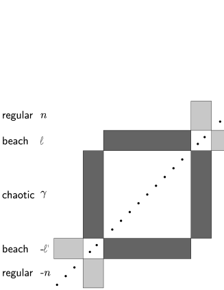
FIG. 6.: The modified block-matrix model: structure of blocks participating in the recer contributions.

We now explain how the properties of $\tilde{S}$ can be extracted from the original matrix $S$. Note that a block that is almost diagonal $\tilde{S}$ will be changed only little in the transformation to $S$. The outermost regular blocks are diagonal in all orders of $1/k$ (or $\hbar$), and matrix elements of the transformed matrix will differ from the original ones only by exponentially small corrections. We can therefore approximate $\tilde{S}_{n,n^{\prime}}\approx S_{n,n}\,\delta_{n,n^{\prime}}$. The argument also holds for the edge region, since the choice of basis for the regular blocks will also be good in the edge blocks, and we can approximate $\tilde{S}_{\ell,\ell^{\prime}}\approx S_{\ell,\ell}\,\delta_{\ell,\ell^{\prime}}$ and in the non-diagonal block $\tilde{S}_{n,\ell}\approx S_{n,\ell}$. Consequently, the choice of the border index between regular and edge blocks does not affect the results to the present approximation.

We model quantum dynamics within the inner block by a superposition of two Gaussian ensembles [39, 40, 29] — in our case two Circular Orthogonal Ensembles (COE) [41] — that approximate the sets of chaotic states with even and odd symmetry, respectively. For a given regular mode $n$ coupling matrix elements $\tilde{S}_{n,\gamma}$ are chosen as Gaussian distributed independent random variables of variance determined by $\sigma^{2}_{n,\text{C}}=|\tilde{S}_{n,\text{C}}|^{2}/(2\ell_{\text{COE}}+1)$ with

$$|\tilde{S}_{n,\text{C}}|^{2}=\sum_{g=-\ell_{\text{COE}}}^{\ell_{\text{COE}}}|S_{n,g}|^{2}\ ,$$ (34)

where we have taken the chaotic block to extend from $\ell_{\text{COE}}$ to $-\ell_{\text{COE}}$. Coupling matrix elements $\tilde{S}_{\ell,\gamma}$ are defined analogously,

$$|\tilde{S}_{\ell,\text{C}}|^{2}=\sum_{g=-\ell_{\text{COE}}}^{\ell_{\text{COE}}}|S_{\ell,g}|^{2}\ ,$$ (35)

The choice of $\ell_{\text{COE}}$ contains some uncertainty that will affect the results as an overall factor in the effective coupling elements. Note that an approximation for single coupling matrix elements $\tilde{S}_{n,\gamma}$, $\tilde{S}_{\ell,\gamma}$ in terms of the original $S$-matrix elements — or, even more, as a semiclassical expression — is presently not possible, as too little is known about the precise nature of the quantum localization on the beach layer. Also, standard semiclassical methods break down in the beach.

For the brevity of notation, we will drop the tildes on $\tilde{S}$ and $\tilde{\theta}$.

C Extracting the Shift, Splitting and Eigenvector Structure

We now use the block matrix model and formulas (31,32) to extract approximations for the shift and the splitting of eigenphase doublets. Also, we comment on how to extract eigenvector structure and to calculate eigenphase properties from it.

1 Eigenphase Splitting

When using Eq. (32) and the block matrix representation of $S$ to calculate the splitting, we have to perform the sum over paths

$\displaystyle{\cal P}^{N}_{n,-n}\,\equiv\,{\sum_{\{n\>\rightarrow-n\}}}\prod_{i=1}^{N-1}\>S_{\lambda_{i},\lambda_{i+1}}$

of length $N\gg\kappa/|\delta\theta_{n}|$. As $N$ is large (and under the assumption that none of the internal diagonal elements $S_{\lambda_{i},\lambda_{i}}$ is equal to $S_{n,n}$) it is sufficient to collect contributions that are of order $N$. We consider three families of paths: paths of type regular-regular (rr) that contain one single jump from $n$ to $-n$, paths of type regular-chaotic-regular (rcr) that pass through the center block, and paths regular-edge-chaotic-edge-regular (recer) that pass through all five blocks. Adding up the different contributions gives the eigenphase splitting as a sum

$$\delta\theta_{n}\approx\delta\theta_{n}^{(rr)}+\delta\theta_{n}^{(rcr)}+\delta\theta_{n}^{(recer)}\ .$$ (36)

Within each of these families, one has to sum over indices of staying times of the path at each diagonal element. We show in Appendix A how this can be done and quote the result: The sum over paths with $M+1$ jumps passing through $M$ intermediate blocks $S^{(i_{1},i_{1})},\ldots,S^{(i_{M},i_{M})}$ is given as

$${\cal P}_{n,-n}^{N\,(i_{1},\ldots,i_{M})}$$ (37)

$$\sim N\mbox{\rm e}\,^{i(N-1)\theta_{n}^{\,(0)}}\sum_{\lambda_{1},\ldots,\lambda_{M}}S_{n,\lambda_{1}}\prod_{i=1}^{M}\frac{S_{\lambda_{i},\lambda_{i+1}}}{\mbox{\rm e}\,^{i\theta_{n}^{\,(0)}}-\mbox{\rm e}\,^{i\theta_{\lambda_{i}}}}\ ,$$ (38)

where the sums over the $\lambda_{\nu}$ run over all indices of the corresponding blocks $S^{(i_{\nu},i_{\nu})}$, and $\lambda_{M+1}=-n$. Corrections to (38) are of lower order in $N$ or higher order in transition amplitudes. The phase denominators

$\displaystyle\mbox{\rm e}\,^{i\theta_{n}^{\,(0)}}-\mbox{\rm e}\,^{i\theta_{\lambda_{i}}}\>\equiv\>d_{n,\lambda_{i}}$

arise from the summation over staying times $T_{i}$ at the different blocks. Within a given family, each path contributes a factor $\exp[iT_{i}(\theta_{\lambda_{i}}-\theta_{n}^{\,(0)})]$, and geometrical summation over $T_{i}$ results in the denominators listed. Note that only phase differences appear that combine the outermost phase $\theta_{n}^{\,(0)}$ with one of the phases $\theta_{\lambda_{i}}$ of the inner blocks. Contributions containing other phase denominators decay exponentially in $N$. Also, we have only taken into account paths that pass through each of the inner blocks once. This “never look back” approximation is justified since paths containing loops are of higher order in the inter-block transition elements. For a treatment of loops in index space, see Appendix A.

Let us now discuss the contributions of the different families in turn. For paths of type regular-regular, we apply Eq. (38) for $M=0$ and find

$$\delta\theta_{n}^{\,(rr)}\>\approx\>2\mathop{\Im{\rm m}}\nolimits\{\mbox{\rm e}\,^{-i\theta_{n}^{\,(0)}}\,{S_{n,-n}}\}\sim\mid S_{n,-n}\mid\ .$$ (40)

Chaos-assisted paths of type regular-chaotic-regular visit the center block. By application of Eq. (38) for $M=1$, we find that the rcr-contribution to the splitting is

$$\delta\theta_{n}^{\,(rcr)}\>\approx\>2\mathop{\Im{\rm m}}\nolimits\Big{\{}\mbox{\rm e}\,^{-i\theta_{n}^{\,(0)}}\sum_{\gamma}\frac{S_{n,\gamma}\,S_{\gamma,-n}}{d_{n,\gamma}}\Big{\}}\ .$$ (41)

Finally, the paths regular-edge-chaotic-edge-regular pass through three intermediate blocks ($M=3$), hence

$$\delta\theta_{n}^{\,(recer)}=2\mathop{\Im{\rm m}}\nolimits\Big{\{}\mbox{\rm e}\,^{-i\theta_{n}^{\,(0)}}\sum_{\gamma,\ell,\ell^{\prime}}\frac{S_{n,\ell}}{d_{n,\ell}}\frac{S_{\ell,\gamma}\,S_{\gamma,-\ell^{\prime}}}{d_{n,\gamma}}\frac{S_{-\ell^{\prime},-n}}{d_{n,\ell^{\prime}}}\Big{\}}\ .$$ (42)

One sees that all tunneling rates mediated by internal blocks can be strongly enhanced by two effects.

(1) Combinations of tunneling matrix elements may become progressively more advantageous as more steps are allowed.

(2) Coherent summation over staying times results in phase denominators. Avoided crossings of these phases turn the splittings into a rapidly fluctuating quantity with respect to small changes in energy, say, or an external parameter of the system. The phase denominators also lead to an overall increase in the tunneling rate since, at a given wave number $k$, there are of order $k$ internal states available. This means that typically, there will be one phase denominator of size $d_{n,\gamma}^{-1}\sim k/2\pi$ at least.

Both effects, (1) and (2), can also enhance the recer contributions with respect to the rcr ones. We can therefore expect the recer contributions to dominate the tunneling rate. For a given system, their relative importance may vary, depending on the size of $|S_{n,\gamma}|$ and $|S_{n,\ell}S_{\ell,\gamma}/d_{n,\ell}|$.

2 Eigenphase Shift

Paths that contribute to the real part of the shift lead from $n$ back to $n$ and have to leave this index at least once. To do so, they can either tunnel to the center block or to the edge block, which leads to a decomposition of contributions into

$\displaystyle\Delta\theta_{n}^{\,(R)}\>\approx\>\Delta\theta_{n}^{(rer)}+\Delta\theta_{n}^{(rcr)}+\Delta\theta_{n}^{(recer)}\ .$

The summation over these paths can be done by the same procedure used above, and one finds that the contributions to the real part of the shift are

$$\Delta\theta_{n}^{\,(rer)} = \mathop{\Im{\rm m}}\nolimits\Big{\{}\mbox{\rm e}\,^{-i\theta_{n}^{\,(0)}}\sum_{\ell}\frac{S_{n,\ell}\,S_{\ell,n}}{d_{n,\ell}}\Big{\}}\ ,\!\!\!$$ (44)

$$\Delta\theta_{n}^{\,(rcr)} = \mathop{\Im{\rm m}}\nolimits\Big{\{}\mbox{\rm e}\,^{-i\theta_{n}^{\,(0)}}\sum_{\gamma}\frac{S_{n,\gamma}\,S_{\gamma,n}}{d_{n,\gamma}}\Big{\}}\ ,\!\!\!$$ (45)

$$\Delta\theta_{n}^{\,(recer)} = \mathop{\Im{\rm m}}\nolimits\Big{\{}\mbox{\rm e}\,^{-i\theta_{n}^{\,(0)}}\sum_{\gamma,\ell,\ell^{\prime}}\frac{S_{n,\ell}\,S_{\ell,\gamma}\,S_{\gamma,\ell^{\prime}}\,S_{\ell^{\prime},n}}{d_{n,\ell}\,d_{n,\gamma}\,d_{n,\ell^{\prime}}}\Big{\}}\ .\!\!\!$$ (46)

Due to the rapid decay of tunneling matrix elements we expect that $|\Delta\theta_{n}^{\,(rer)}|\gg|\Delta\theta_{n}^{\,(recer)}|\gtrsim|\Delta\theta_{n}^{\,(rcr)}|$. Furthermore from Eqs. (42,46), $|\Delta\theta_{n}^{\,(recer)}|\simeq|\delta\theta_{n}^{\,(recer)}|$. Consequently, the shift will typically be much larger than the splitting.

3 Eigenvectors

We can also use the block matrix model to approximate regular eigenvector doublets $\mathchoice{{\hbox{\boldmath$\displaystyle\alpha$}}}{{\hbox{\boldmath$\textstyle\alpha$}}}{{\hbox{\boldmath$\scriptstyle\alpha$}}}{{\hbox{\boldmath$\scriptscriptstyle\alpha$}}}^{\pm}$. We set $\alpha^{\pm}_{n}=1/\sqrt{2}$ and $\alpha^{\pm}_{-n}=\pm 1/\sqrt{2}$, and solve

$\displaystyle(S-\mbox{\rm e}\,^{i\theta_{n}^{\pm}})\,\mathchoice{{\hbox{\boldmath$\displaystyle\alpha$}}}{{\hbox{\boldmath$\textstyle\alpha$}}}{{\hbox{\boldmath$\scriptstyle\alpha$}}}{{\hbox{\boldmath$\scriptscriptstyle\alpha$}}}^{\pm}=0$

to leading order in the coupling matrix elements between neighboring blocks (neglecting all other coupling matrix elements). We find that the components of $\mathchoice{{\hbox{\boldmath$\displaystyle\alpha$}}}{{\hbox{\boldmath$\textstyle\alpha$}}}{{\hbox{\boldmath$\scriptstyle\alpha$}}}{{\hbox{\boldmath$\scriptscriptstyle\alpha$}}}^{\pm}$ in the beach regions are

$$\alpha_{\ell}^{\pm}\approx\frac{1}{\sqrt{2}}\,\frac{S_{n,\ell}}{d_{n,\ell}}\;$$ (48)

and $\alpha^{\pm}_{-\ell}=\pm\alpha^{\pm}_{\ell}$. Components in the center block are given by

$$\alpha_{\gamma}^{\pm}=\frac{\sqrt{2}}{d_{n,\gamma}}\sum_{\ell}\frac{S_{n,\ell}\,S_{\ell,\gamma}}{d_{n,\ell}}=\sigma_{\gamma}\sum_{\ell^{\prime}}\frac{\sqrt{2}}{d_{n,\gamma}}\frac{S_{\gamma,-\ell^{\prime}}\,S_{-\ell^{\prime},-n}}{d_{n,\ell}}\ ,$$ (49)

if the symmetry $\sigma_{\gamma}\in\{\pm 1\}$ of the block-diagonalizing vector $|\gamma\rangle$ is the same as that of $\mathchoice{{\hbox{\boldmath$\displaystyle\alpha$}}}{{\hbox{\boldmath$\textstyle\alpha$}}}{{\hbox{\boldmath$\scriptstyle\alpha$}}}{{\hbox{\boldmath$\scriptscriptstyle\alpha$}}}^{\pm}$, and $\alpha_{\gamma}^{\pm}=0$ otherwise. In both Eqs. (49) the relative error is ${\cal O}(|S_{n,\ell}|^{2}/d_{n,\ell},|S_{\ell,\gamma}|^{2}/d_{n,\gamma})$.

This approximation for the eigenvectors can be used to relate eigenphase properties to the size of eigenvector components in the different blocks. Upon comparison of Eqs. (44) and (48), we see that the dominant contribution to the shift can be written as

$$\Delta\theta_{n}^{\,(rer)}=2\mathop{\Im{\rm m}}\nolimits\Big{\{}\sum_{\ell}\mbox{\rm e}\,^{-i\theta_{n}^{\,(0)}}\,d_{n,\ell}\>(\alpha_{\ell})^{2}\Big{\}}\ ,$$ (50)

where $\textstyle\alpha$ is either of the $\mathchoice{{\hbox{\boldmath$\displaystyle\alpha$}}}{{\hbox{\boldmath$\textstyle\alpha$}}}{{\hbox{\boldmath$\scriptstyle\alpha$}}}{{\hbox{\boldmath$\scriptscriptstyle\alpha$}}}^{\pm}$. Therefore, the eigenphase shift is related to the eigenvector’s overlap with the beach region. Similarly, from Eqs. (42) and (49),

$$\delta\theta_{n}^{\,(recer)}=\mathop{\Im{\rm m}}\nolimits\Big{\{}\sum_{\gamma}\mbox{\rm e}\,^{-i\theta_{n}^{\,(0)}}\,d_{n,\gamma}\>[(\alpha^{+}_{\gamma})^{2}-(\alpha^{-}_{\gamma})^{2}]\Big{\}}\ .$$ (51)

Eq. (51) relates the presumably dominant contribution to the splitting to the eigenvector’s overlap with the center block. This explains and quantifies the observation of Utermann et al. [7], that regular doublet splittings in a mixed system are in close correlation with the states’ projection onto the chaotic sea. Similarly, Gerwinski and Seba [42] related tunneling rates between a chaotic phase space region and a regular island to the overlap of a chaotic scattering state with the regular island. However, we see that the ad hoc association

$$|\,\Delta\theta_{n}|\sim\sum_{\ell}\,|\,\alpha_{\ell}\,|^{2}\ ,\qquad|\,\delta\theta_{n}|\sim\sum_{\gamma}|\,\alpha_{\gamma}\,|^{2}$$ (52)

is not complete: in the exact relation (51), each summand is weighted by a phase difference.

4 Comments

In view of the explicit formulas, we see that the results are not significantly changed by approximating the regular and edge blocks of $\tilde{S}$ by the corresponding elements of the original matrix $S$. Only in the immediate vicinity of resonances between regular and beach eigenphases the approximation $\tilde{S}_{\ell,\ell}\approx S_{\ell,\ell}$ is not appropriate, as it over-estimates the imaginary part of the phase $\theta_{\ell}$ and leads to a spuriously broad resonance. (With the neglect of $\Delta\theta_{\ell}^{\,(R)}$ we shall not be concerned, because we do not aim at an exact reproduction of the peak positions.) For most beach states, it is therefore more appropriate to make the somewhat ad hoc approximation of $\theta_{\ell}=\arg\{S_{\ell,\ell}\}$ instead of $-i\log S_{\ell,\ell}$. This approximation now leads to an under-estimate of the resonance width, but we have checked that in the cases discussed in Section IV D the edge $\ell$ are sufficient large ($\ell\geq 59$) that the resonances $|S_{n,n}-\tilde{S}_{\ell,\ell}|^{-1}$ and $|S_{n,n}-\exp(i\theta_{\ell})|^{-1}$ cannot be distinguished by eye.

From a methodological point of view, it is worthwhile mentioning that the formulas for the shift and the splitting can also be derived from a complementary approach. One can expand the characteristic polynomial

$\displaystyle P_{S}(x)=\det(S-x)$

of $S$ around $x_{n}=\exp(i\theta_{n}^{\,(0)})$ to second order in the external coupling elements $|S_{n,\lambda_{1}}|$, $|S_{\lambda_{M},-n}|$, and then solve for its roots $x^{\pm}$, $P_{S}(x^{\pm})=0$. Upon definition of shift and splitting via $x^{\pm}=x_{n}+\Delta x\pm\delta x/2$, one finds formulas that, to lowest order in the internal coupling elements, are identical to Eqs. (42, 44). Hence, the “never look back” summation over paths corresponds to the lowest order of a formal expansion of the eigenvalues, containing the coupling elements as small parameters.

It is important to realize that the different phase denominators $d_{n,\ell}$ and $d_{n,\gamma}$ may fluctuate on different scales as functions of the energy or an external parameter. Typically, the center block will be much larger than the beach blocks, and avoided crossings of $\theta_{n}^{\,(0)}$ with one of the $\theta_{\gamma}$ will occur more often than those with one of the $\theta_{\ell}$. Also, since beach states display EBK-like behavior with actions that can be similar to those of the regular states, we can expect phase differences $\theta_{n}^{\,(0)}-\theta_{\ell}$ to vary more slowly than phase differences $\theta_{n}^{\,(0)}-\theta_{\gamma}$. (For the case of the annular billiard, a semiclassical argument is given in Ref. [23].) Consequently, eigenphase splittings $\delta\theta_{n}^{\,(recer)}$ will show fluctuations on two scales: There will be a rapid sequence of peaks due to avoided crossings of regular eigenphases with chaotic ones and a slow modulation due to the relative motion of regular and beach eigenphases.

Let us conclude by summarizing those predictions that genuinely depend on the explicit inclusion of the beach layers into the five-block matrix model:

(I) Eigenphase splitting: Contributing paths typically pass through all blocks. As a function of an external parameter, the splitting varies on two scales: a slow one attributed to the change of the $d_{n,\ell}^{-2}$, and a rapid one attributed to the change of the $d_{n,\gamma}^{-1}$. Consequently, one sees resonances of different line shapes.

(II) Eigenphase shift: Paths contributing to the shift typically visit only the beach layer. The shift is much larger than the splitting, and it varies with $d_{n,\ell}^{-1}$ on the slow scale only.

None of these statements would hold for the three-block model, and therefore (I) and (II) can serve as a test of our five-block model.

D Numerical Results

We now give numerical examples of the formulas just presented. In particular, we will give the most quantitative and direct proof of the chaos-assisted tunneling picture yet. Also, we will test the predictions derived from the explicit treatment of the beach layer in our five-block matrix model. Again, we consider the annular billiard at parameter values $k=100$, $a=0.4$ and $\delta=0.2$.

First of all, we have to decide on where to set the borders between the different blocks. As was already mentioned, the outer borders between the regular blocks and the edge blocks do not pose any problem as in both blocks, matrix elements are approximated by the corresponding matrix elements of the original $S$-matrix. Due to the tunneling ridges in the region $\ell\gtrsim k(a+\delta)$, paths starting from high $n$ will most likely tunnel into this region first. In order to include these paths, we extend the beach region into the regular block whenever necessary.

The border between the beach region and the chaotic block is more difficult to determine. In Section IV E we give numerical evidence that some of the beach states’ structure arises from trapping of classical motion near KAM-like regular island extending into the chaotic sea down to impact parameters $|L|\approx 0.55$. This would suggest the choice of $|\ell|=55$ for the borders between the edges and the chaotic block. However, chaotic states that can carry transport between positive and negative angular momenta have sizeable overlap only with angular momentum components between $\ell=-50$ and $\ell=50$. Therefore, we will take the chaotic block to extend over

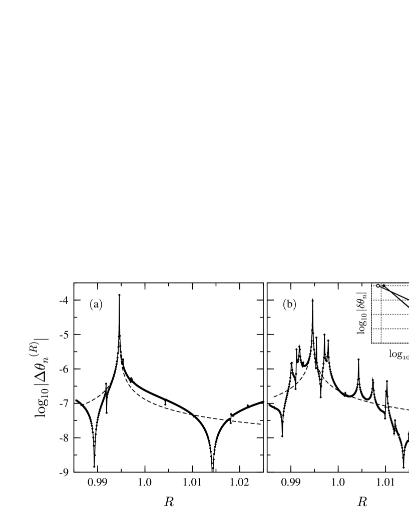
FIG. 7.: (a) Eigenphase shift $\Delta\theta_{n}^{\,(R)}$ and (b) splitting $\delta\theta_{n}$ of the doublet $n=70$ for different values of the radius $R$ of the outer circle: exact results as obtained by numerical diagonalization (circles) and contribution predicted by the block matrix model that is dominant between $R\approx 0.99$ and $R\approx 1.015$ (dashed line, see text). Inset: power law dependence of splitting near $R_{p}=0.9946$ (full circles) and $R_{p}=1.0043$ (empty circles). Throughout, full lines are to guide the eye.

angular momenta $|\ell|\leq\ell_{\text{COE}}=50$. The uncertainty inherent in the choice of $\ell_{\text{COE}}$ affects the final results via the effective couplings $S_{\ell,\gamma}$, $S_{n,\gamma}$ which can therefore only be determined up to an overall constant of order one.

Let us briefly discuss the magnitudes of the tunneling amplitudes involved in the different contributions to the splitting. As expected, the direct $n$ to $-n$ tunneling matrix element is of negligible size. At the present parameter values $\delta\theta_{70}^{\,(rr)}\sim|S_{70,-70}|\sim 10^{-60}$ which is by many orders of magnitude smaller than the observed splitting $\delta\theta_{70}\sim 10^{-10}$. The difference between contributions $\delta\theta_{n}^{\,(rcr)}$ and $\delta\theta_{n}^{\,(recer)}$ is less drastic. At the parameter values considered, effective coupling elements $S_{n,\ell}S_{\ell,\gamma}/d_{n,\gamma}$ are usually by at least an order of magnitude larger than the corresponding $S_{n,\gamma}$.

The dominance of recer contributions is particularly clear when studying the behavior of shift and splitting as a function of an external parameter. We show in Fig. 7 the shift and the splitting of the doublet $n=70$ as obtained from numerical diagonalization of the $S$-matrix as a function of the outer circle’s radius $R=0.985$–$1.025$. $R$ varies over a sufficiently small interval as to leave the classical billiard dynamics essentially unchanged. The choice of $R$ as external parameter has the advantage that the tunneling magnitudes given by the inner scattering matrix $|S_{n,\ell}|=|S^{\,\text{(I)}}_{n,\ell}|$ remain constant, as variation of $R$ affects only the outer scattering matrix $S^{\,\text{(O)}}$.

Fig. 7(a) displays the real part of the shift $\Delta\theta_{n}^{\,(R)}$. The shift varies slowly as a function of $R$ and is over long ranges well reproduced by just a single term of Eq. (42). (The dashed line shows $|S_{70,59}^{2}/d_{70,59}|$ with

$d_{70,59}\approx\theta_{70}^{\,(0)}-\theta_{59}$ extracted from $S$, slightly shifted to account for $\Delta\theta_{59}$.) Over relatively large ranges of $R$, one single $\ell$ is clearly dominant. Transitions between domains of different dominant $\ell$ are marked by very small shifts due to cancelations between contributing paths. Fig. 7(b) shows the splitting of the same doublet. Note that the logarithmic scale in plot (b) ranges over twice the number of orders of magnitude than in (a). As predicted by the five-block model, the splitting is much smaller than the shift and shows variations on two scales. The overall, slow modulation is determined by the beach resonance $\propto d_{70,59}^{-2}$ and closely follows the behavior of the shift. On top of this modulation lies a rapid sequence of spikes that we attribute to quasi-crossings with eigenphases of the internal block.

For the $\ell=59$ contribution to the splitting (dashed line), we used Eq. (80) of the next Section to estimate the median taken over the properties of the chaotic block and divided out a factor $\sim 15$ to make the dashed line coalesce with the splitting away from the $d_{n,\gamma}$-resonances. Note that the change of dominant edge index $\ell$ is signaled by a strong cancelation of tunneling paths. In the inset, we compare the line shapes of the two types of resonances by plotting $|\delta\theta_{70}|$ as a function of $|R-R_{p}|$ in a double logarithmic plot near the “beach” peak ($R_{p}=0.9946$, full circles) and a “chaotic” peak ($R_{p}=1.0043$, empty circles). Power laws with exponents $-2$ and $-1$ are obeyed to good precision, thus confirming the prediction of the five-block model.

It is evident that the predictions of the five-block model serve very well to explain the data. We stress again that the effects just described — different line shapes and fluctuations on two parameter scales — genuinely depend on the role of the beach layer in tunneling processes. They serve as clear fingerprints of the quantum implications of the presence of an beach layer between phase space regions of classically regular and chaotic motion.

Let us however mention that the correspondence between shift and splitting can be less clear. For large $n$ the shift can show additional modulations that do not appear in the splitting whenever there is a degeneracy with an beach mode with large $\ell$ [32]. In the shift, this resonance is weighted with $|S_{n,\ell}|^{2}$, which favors $\ell$ near the tunneling ridge. In the splitting, the resonance’s contribution has the weight $|S_{n,\ell}S_{\ell,\gamma}|^{2}$ which can become very small if $\ell$ is too large. This does however not contradict the predictions (I) and (II), it merely means that shift and splitting arise by coupling to different beach modes.

For later purposes it is important to note that whenever the same beach state is dominant in both shift and splitting, the correspondence between the shift and the slow modulations of the splitting can be used to “unfold” the splitting data from beach properties. By Eqs. (42,44), the ratio

$$\widetilde{\delta\theta}_{n}=\frac{4}{\pi}\frac{\delta\theta_{n}}{[\Delta\theta_{n}^{\,(R)}]^{2}}\left|\frac{S_{n,\ell}}{S_{\ell,C}}\right|^{2}\sim\frac{1}{{|S_{l,\text{C}}|^{2}}}\left|\sum_{\gamma}\frac{S_{\ell,\gamma}\,S_{\gamma,-\ell}}{d_{n,\gamma}}\right|$$ (53)

then contains only properties of the center block and can therefore be used to extract its “bare” quantities.

E Evolution of Tunneling Flux on the PSOS

Let us recall that the scattering matrix $S$ is the quantum analogue of the classical Poincaré mapping; it constitutes a time domain-like propagator in the representation fixed by Eq. (4). This makes it possible to study the evolution of ”wave packets” — vectors $\mathchoice{{\hbox{\boldmath$\displaystyle\alpha$}}}{{\hbox{\boldmath$\textstyle\alpha$}}}{{\hbox{\boldmath$\scriptstyle\alpha$}}}{{\hbox{\boldmath$\scriptscriptstyle\alpha$}}}_{0}$ corresponding to initial conditions localized in phase space — under the action of $S$. In particular, it is here of interest to follow the evolution of a tunneling process in phase space.

The comparison of quantum dynamics and classical phase space can, in the context of the scattering approach to quantization, conveniently be done by use of Wigner- and Husimi-like functions of quantum operators [43, 23]. Let ${\cal A}$ be some operator that, for definiteness, we represent in angular momentum basis. As explained in detail in Ref. [23], ${\cal A}$ can be transformed to a function $\rho^{\text{H}}[{\cal A}](\gamma,L)$ on the Poincaré cell ${\cal C_{P}}$ by first performing a Wigner-transform on ${\cal A}$ and then smoothing with a minimal-uncertainty wave packet. One obtains

$$\rho^{\text{H}}[{\cal A}](\gamma,L)=\sum_{\ell\ell^{\prime}}{\cal A}_{\ell,\ell^{\prime}}\times$$ (54)

$$\exp\left\{\frac{-\Delta\gamma^{2}}{2}\left[\left(kL-\frac{\ell+\ell^{\prime}}{2}\right)^{2}+(\ell-\ell^{\prime})^{2}\right]-i\gamma(\ell-\ell^{\prime})\right\}\ ,$$ (55)

where $(\gamma,L)$ are the coordinates in ${\cal C_{P}}$, $k$ is the wave number, and $\Delta\gamma^{2}$ is a parameter determining the shape of the smoothing wave packet. We choose $\Delta\gamma^{2}=4/k$. In case that ${\cal A}=\mathchoice{{\hbox{\boldmath$\displaystyle\alpha$}}}{{\hbox{\boldmath$\textstyle\alpha$}}}{{\hbox{\boldmath$\scriptstyle\alpha$}}}{{\hbox{\boldmath$\scriptscriptstyle\alpha$}}}\cdot\mathchoice{{\hbox{\boldmath$\displaystyle\alpha$}}}{{\hbox{\boldmath$\textstyle\alpha$}}}{{\hbox{\boldmath$\scriptstyle\alpha$}}}{{\hbox{\boldmath$\scriptscriptstyle\alpha$}}}^{\dagger}$ is the projector of a (normalized) vector $\alpha$, its transform $\rho^{\text{H}}_{\mathchoice{{\hbox{\boldmath$\displaystyle\alpha$}}}{{\hbox{\boldmath$\textstyle\alpha$}}}{{\hbox{\boldmath$\scriptstyle\alpha$}}}{{\hbox{\boldmath$\scriptscriptstyle\alpha$}}}}(\gamma,L)$ constitutes a positive semi-definite, normalized density distribution on the Poincaré cell, the Husimi Poincaré Density (HPD). By use of HPDs, it becomes possible to follow the phase space evolution of a tunneling process from one regular torus to its counterpart. The “dynamics” (in iteration count $N$ as the time variable) of such a process is visualized by projecting iterates $\mathchoice{{\hbox{\boldmath$\displaystyle\omega_{N}$}}}{{\hbox{\boldmath$\textstyle\omega_{N}$}}}{{\hbox{\boldmath$\scriptstyle\omega_{N}$}}}{{\hbox{\boldmath$\scriptscriptstyle\omega_{N}$}}}=S^{N}\mathchoice{{\hbox{\boldmath$\displaystyle\omega$}}}{{\hbox{\boldmath$\textstyle\omega$}}}{{\hbox{\boldmath$\scriptstyle\omega$}}}{{\hbox{\boldmath$\scriptscriptstyle\omega$}}}_{0}$ of some initial vector $\mathchoice{{\hbox{\boldmath$\displaystyle\omega$}}}{{\hbox{\boldmath$\textstyle\omega$}}}{{\hbox{\boldmath$\scriptstyle\omega$}}}{{\hbox{\boldmath$\scriptscriptstyle\omega$}}}_{0}$ onto ${\cal C_{P}}$.

Returning to the annular billiard, we consider a starting vector $\mathchoice{{\hbox{\boldmath$\displaystyle\omega$}}}{{\hbox{\boldmath$\textstyle\omega$}}}{{\hbox{\boldmath$\scriptstyle\omega$}}}{{\hbox{\boldmath$\scriptscriptstyle\omega$}}}_{0}$ peaked at high angular momentum $n$ and calculate the Husimi densities $\rho^{\text{H}}[\langle\mathchoice{{\hbox{\boldmath$\displaystyle\omega$}}}{{\hbox{\boldmath$\textstyle\omega$}}}{{\hbox{\boldmath$\scriptstyle\omega$}}}{{\hbox{\boldmath$\scriptscriptstyle\omega$}}}_{N}\cdot\mathchoice{{\hbox{\boldmath$\displaystyle\omega$}}}{{\hbox{\boldmath$\textstyle\omega$}}}{{\hbox{\boldmath$\scriptstyle\omega$}}}{{\hbox{\boldmath$\scriptscriptstyle\omega$}}}_{N}^{\dagger}\rangle]$ of averaged autocorrelations

$$\langle\>\mathchoice{{\hbox{\boldmath$\displaystyle\omega$}}}{{\hbox{\boldmath$\textstyle\omega$}}}{{\hbox{\boldmath$\scriptstyle\omega$}}}{{\hbox{\boldmath$\scriptscriptstyle\omega$}}}_{N}\cdot\mathchoice{{\hbox{\boldmath$\displaystyle\omega$}}}{{\hbox{\boldmath$\textstyle\omega$}}}{{\hbox{\boldmath$\scriptstyle\omega$}}}{{\hbox{\boldmath$\scriptscriptstyle\omega$}}}_{N}^{\dagger}\>\rangle\>=\>\sum_{M=0}^{50}\tilde{\mathchoice{{\hbox{\boldmath$\displaystyle\omega$}}}{{\hbox{\boldmath$\textstyle\omega$}}}{{\hbox{\boldmath$\scriptstyle\omega$}}}{{\hbox{\boldmath$\scriptscriptstyle\omega$}}}}_{N+M}\cdot\tilde{\mathchoice{{\hbox{\boldmath$\displaystyle\omega$}}}{{\hbox{\boldmath$\textstyle\omega$}}}{{\hbox{\boldmath$\scriptstyle\omega$}}}{{\hbox{\boldmath$\scriptscriptstyle\omega$}}}}_{N+M}^{\dagger}$$

FIG. 8.: Spread of tunneling flux over the chaotic sea: build-up of quantum amplitude in the beaches. Grayscale plots (arbitrary scale) of averaged autocorrelations of the (a) 50-th, (b) 100-th, and (c) 500-th iterate of a vector peaked at $n=66$. The initial component $n$ has been left out. Full lines indicate classical tori.

in which the mean over 50 iterations has been performed in order to average out the internal dynamics of the center block. The tilde indicates that the $n$-th component of $\textstyle\omega$ has been set to zero. (This truncation is necessary because the smoothing tails of the large $n$-th component would obscure all features in the nearby beach regions.)

Fig. 8 depicts the flow of tunneling probability on ${\cal C_{P}}$ by showing $\rho^{\text{H}}[\langle\mathchoice{{\hbox{\boldmath$\displaystyle\omega$}}}{{\hbox{\boldmath$\textstyle\omega$}}}{{\hbox{\boldmath$\scriptstyle\omega$}}}{{\hbox{\boldmath$\scriptscriptstyle\omega$}}}_{N}\cdot\mathchoice{{\hbox{\boldmath$\displaystyle\omega$}}}{{\hbox{\boldmath$\textstyle\omega$}}}{{\hbox{\boldmath$\scriptstyle\omega$}}}{{\hbox{\boldmath$\scriptscriptstyle\omega$}}}_{N}^{\dagger}\rangle]$ for $n=66$ and $N=50$, $100$ and $500$. At these parameter values, the tunneling period between WG tori is $2\pi/\delta\theta_{66}\sim 10^{7}$. As predicted by the five-block matrix model, probability is fed from the starting angular momentum $n$ into the nearby beach region until it reaches a value $\sim|S_{n,\ell}|^{2}$ ($\ell=58$) and spreads over the chaotic sea up to a value $\sim|S_{n,\ell}S_{\ell,\text{C}}|^{2}$, see Fig. 8(a). Oscillations between the beaches set in with period $2\pi/\delta\theta_{58}\sim 1000$, see Fig. 8(b,c). On a much larger time scale, probability amplitude starts to build up at at $-n$ (not shown here). One clearly sees that the shape of the HPD is structured by the underlying classical dynamics: in the beaches, most probability builds up around the chains of small KAM-like islands, whereas in the chaotic sea, the center island and its satellites are not penetrated. Also, the regions around the satellite islands and the homoclinic tangles between them are filled only weakly.

Chaotic phase space can also be filled in a different manner, depending on the phases $\theta_{n}$, $\theta_{\ell}$ and $\theta_{\gamma}$ involved in the tunneling process. In Fig. 9 we present the case of a close degeneracy between $\theta_{n}$ and one of the $\theta_{\gamma}$. We show $\langle\mathchoice{{\hbox{\boldmath$\displaystyle\omega$}}}{{\hbox{\boldmath$\textstyle\omega$}}}{{\hbox{\boldmath$\scriptstyle\omega$}}}{{\hbox{\boldmath$\scriptscriptstyle\omega$}}}_{N}\cdot\mathchoice{{\hbox{\boldmath$\displaystyle\omega$}}}{{\hbox{\boldmath$\textstyle\omega$}}}{{\hbox{\boldmath$\scriptstyle\omega$}}}{{\hbox{\boldmath$\scriptscriptstyle\omega$}}}_{N}^{\dagger}\rangle$ for $N=4000$ and the starting vector $\mathchoice{{\hbox{\boldmath$\displaystyle\omega$}}}{{\hbox{\boldmath$\textstyle\omega$}}}{{\hbox{\boldmath$\scriptstyle\omega$}}}{{\hbox{\boldmath$\scriptscriptstyle\omega$}}}_{0}$ peaked at $n=65$. In this case, there is high probability amplitude in the sticking regions around the center satellite islands.

Finally, we present in Fig. 10 HPDs of nine eigenvectors of $S$ at $k=100$, $a=0.4$ and $\delta=0.2$ ($k=100$, one should note, is not an eigenenergy of the annular billiard). By the Weyl formula [44] these vectors would, when quantized at a close-by energy, correspond to the $\sim 2000$-th exited states. We show grayscale plots of HPDs $\rho_{\mathchoice{{\hbox{\boldmath$\displaystyle\alpha$}}}{{\hbox{\boldmath$\textstyle\alpha$}}}{{\hbox{\boldmath$\scriptstyle\alpha$}}}{{\hbox{\boldmath$\scriptscriptstyle\alpha$}}}}^{\text{H}}$ with steps in grayscale corresponding to equidistant probability contour lines. The overall scales vary with each sub-plot. These HPDs at hand, the spread of tunneling amplitude can now be understood in terms of participating eigenvectors. For example, the doublet depicted in (b) and (c) is the beach doublet involved in the tunneling process of Fig. 8. Likewise, the vector (f) peaked around the center satellite islands is the nearly

FIG. 9.: Spread of tunneling flux over the chaotic sea: case of a direct degeneracy between the regular doublet and an internal state. Grayscale plot (arbitrary scale) of averaged autocorrelation of the 4000-th iterate of a vector peaked at $n=65$.

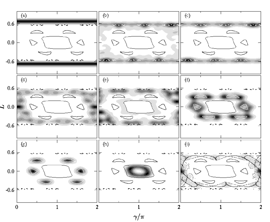
FIG. 10.: Poincaré Husimi Distributions of selected eigenvectors of the annular billiard at $k=100$, $a=0.4$ and $\delta=0.2$. (a) Regular high-angular momentum vector, (b,c) doublet of beach vectors, (d,e) “chaotic” vectors, (f) vector in the sticking region around the satellite islands, (g) regular vector on the period-6 satellite islands, (h) regular vector residing on the main island, and (i) vector scarred by the unstable period-1 fixed point and its homoclinic crossings (dots depict the stable and unstable manifolds).

degenerate one in the tunneling process shown in Fig. 9. Evidently, their shape forms the spread of tunneling probability on the Poincaré cell.

We note that similar figures for much higher wavenumber $k=600$, corresponding to the $\sim 75000$-th excited states, can be found in Ref. [23].

F How Important is Chaoticity?

Let us now discuss a numerical study similar to that performed in the original work by Bohigas et al. [8] in which regular level splittings are calculated as a function of eccentricity $\delta$ at constant $a+\delta$. It is important to note that increasing $\delta$ has two effects: classical motion in the inner layer $|L|<a+\delta$ becomes chaotic, and simultaneously tunneling rates from the regular torus to the chaotic layer are enhanced. A priori, it is not clear which one of these effects governs the rate at which the splittings change, but a quantitative estimate of either effect has now become possible.

We calculated the splittings of high-angular momentum modes for $\delta=0.03$–$0.2$ and $a+\delta=0.6$ at $k=60$. Fig. 11 displays the eigenphase splitting $|\delta\theta_{n}|$ for $n=39$ ($n/k=0.65$). Exact splittings (full lines) increase over eight orders of magnitude and roughly follow an exponential increase with $\delta$. A description of the data in terms of our block-matrix model that reproduces all the fine details might be a difficult task — even with exact $S$-matrix elements at hand — as the model relies on classical information to select the borders between the different blocks and assumes that, apart from the beach layers, no significant phase space structure is present. Therefore, the block-matrix model would have to be adjusted to the varying classical dynamics as $\delta$ changes, and the effect of remaining structure at lower $\delta$ might have to be taken into account with the introduction of different blocks. However, the now-familiar slow modulations in Fig. 11 point to the effect of beach layer states mediating the tunneling flux — however complicated the internal structure might be. Indeed, we find that over the range $\delta=0.07$–0.16 the tunneling processes are mediated by two beach states peaked around $\ell=29$, with $\ell/k=0.48$ well inside the non-integrable regime. In Fig. 11, we have plotted $|S_{n,\ell}|^{2}$ as a dotted line (with arbitrary offset) to give a rough estimate of the change of regular-to-beach tunneling elements via these particular beach states.

FIG. 11.: Eigenphase splitting $|\,\delta\theta_{n}|$ of doublet $n=39$ as a function of eccentricity $\delta$: exact splittings (full line), increase of torus-to-beach tunneling matrix elements ($\ell=29$ dotted line, with arbitrary overall factor), and effect of regular-to-beach phase denominators (dashed line, with arbitrary overall factor). For $\delta>0.15$: tunneling via $\ell=35$ (dashed-dotted line).

Taking into account also the effect of beach denominators, we have plotted $|S_{n,\ell}/d_{n,\ell}|^{2}$ (dashed line). This estimate is multiplied with an overall factor $2\cdot 10^{-5}$ to make the line coincide with the exact data at small $\delta$. The dashed line already gives a fair reproduction of the data. It misses only the sharp peaks due to resonances with the chaotic states, the depression of $\delta\theta_{n}$ between the $d_{n,\ell}^{-2}$ peaks due to destructive interference, and the change of coupling strength of the beach state to the chaotic center states. We conclude that between $\delta=0.07$ and $\delta=0.2$, the splitting is predominantly determined by the change of beach parameters, and that the change of internal coupling between beach and chaotic sea accounts only for a factor of the order $10$ (difference between the dashed line and the exact data at $\delta=0.15$). For larger $\delta$, different beach doublets take over, but the basic structure is preserved. The dashed-dotted line displays the recer-contributions for $\ell=35$ and $\ell_{\text{COE}}=20$.

At $\delta$-values below $0.07$, numerical precision does not allow us to calculate the splitting directly. We can however get an impression by looking at the splitting of states supported by quasi-integrable structures at small $\delta$. Presumably, these states will mediate the tunneling of high-angular momentum doublets. In Fig. 12, we show the splitting of the doublet predominantly peaked at $\ell=27$ ($\ell/k=0.45$). The splitting shows resonance peaks below $\delta\approx 0.075$ and then flattens out. This behavior can be understood by looking at the HPDs of the states involved. In Fig. 13 we depict one partner of the tunneling doublet and its resonant state at (a–c) $\delta=0.0402$, (d–f) $\delta=0.0687$, and (g–h) $\delta=0.09$. In the corresponding classical Poincaré cells, we have started trajectories from initial conditions $(\pi,L)$ with $L>0$ only to indicate the classical inhibition of transport. We can make two interesting observations: First of all, the resonant tunneling process is mediated by regular states residing on the inner island. Resonant tunneling via the center island remains the dominant mechanism, even when classical transport from positive to negative $L$ becomes allowed (d–f). Here, tunneling between a chaotic doublet is mediated by a regular state. Secondly, the outer doublet supported by the KAM-like tori at small $\delta$ evolves into a doublet of states scarred near the unstable periodic orbit and stretched along its stable and unstable manifolds. By quantum localization effects, the doublet structure persists — despite of the seemingly chaotic classical motion (see also [23]). Tunneling between the scarred doublet is direct, as indications of resonances are absent in the splitting beyond $\delta=0.075$.

         

FIG. 12.: Eigenphase splitting of a doublet peaked around $\ell=27$ at $k=60$ as a function of $\delta$. Here, resonances arise from avoided crossings with states residing on the center island.

We are led to the conclusion that the enhancement of tunneling rates between symmetry-related phase space objects ${\cal A}$ and ${\cal T}{\cal A}$ by resonance with quantum states supported by an intervening phase-space structure ${\cal B}$ is only very loosely related to the chaoticity of ${\cal B}$, but rather depends on the topological character of ${\cal B}$. In ${\cal B}$, it must merely be possible to traverse phase space distance in

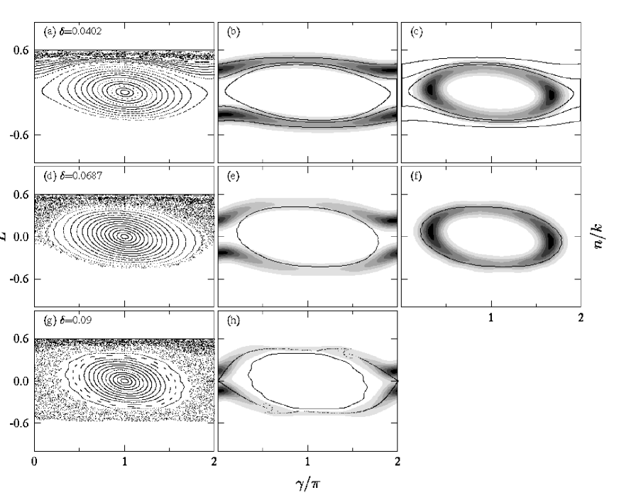
FIG. 13.: Classical phase space and Husimi Poincaré distributions of the tunneling doublet of Fig. 12 and its resonant states at (a–c) $\delta=0.0402$, (d–f) $\delta=0.0687$ and (g–h) $\delta=0.09$. The doublet resides on KAM-like tori for small $\delta$ and dissolves in the chaotic sea for large $\delta$. Note that the tunneling at $\delta=0.0687$ takes place between a chaotic doublet and is mediated by a regular state. At $\delta=0.09$, the dominant tunneling process is direct.

classically allowed steps. It might therefore be more appropriate to refer to “transport-assisted tunneling,” a phenomenon of a more general class than the chaos-assisted tunneling one.

V Statistical Analysis of Eigenphase Splittings

A Asymptotic Behavior of the Splitting Distribution

This Section is devoted to the distribution of level splittings. We determine the asymptotic large-$\delta\theta_{n}$ behavior of the splitting distribution and find “typical” splitting values by calculating the median of the distribution obtained by extrapolation of the asymptotic behavior towards smaller splittings. We assume that recer contributions dominate and that properties of the beach blocks vary slowly. It is straightforward to apply the calculation to the case of rcr contributions as well.

Starting from Eq. (42) we introduce a number of notational simplifications. For a given $n$, we write phases with respect to $\theta_{n}^{\,(0)}$ (that is, set $\theta_{n}^{\,(0)}=0$), define $x_{\gamma}=2\sin(\theta_{\gamma}/2)$ and collect the coupling of $\pm n$ to a chaotic state $\gamma$ via the edge into an effective overlap

$$v_{n,\gamma}=$$ (56)

$$-2\mathop{\Re{\rm e}}\nolimits\Big{\{}\,\sum_{\ell,\ell^{\prime}}\mbox{\rm e}\,^{-i(\theta_{\gamma}+\theta_{\ell}+\theta_{\ell^{\prime}})/2}\>\frac{S_{n,\ell}\,S_{\ell,\gamma}\,S_{\gamma,-\ell^{\prime}}\,S_{-\ell^{\prime},-n}}{2\sin(\theta_{\ell}/2)\,2\sin(\theta_{\ell^{\prime}}/2)}\Big{\}}\ ,$$ (57)

which leads to

$$\delta\theta_{n}^{\,(recer)}\>=\>\sum_{\gamma=1}^{N_{\gamma}}\>\frac{v_{n,\gamma}}{x_{\gamma}}\ .$$

$N_{\gamma}$ denotes the dimension of the center block. In the sequel we drop the subscript $n$.

To devise a statistical treatment for the center block, we make the following assumptions concerning the distribution of the chaotic eigenphases $\mathchoice{{\hbox{\boldmath$\displaystyle\theta$}}}{{\hbox{\boldmath$\textstyle\theta$}}}{{\hbox{\boldmath$\scriptstyle\theta$}}}{{\hbox{\boldmath$\scriptscriptstyle\theta$}}}=\{\theta_{\gamma}\}$, and the effective overlaps $\mathchoice{{\hbox{\boldmath$\displaystyle v$}}}{{\hbox{\boldmath$\textstyle v$}}}{{\hbox{\boldmath$\scriptstyle v$}}}{{\hbox{\boldmath$\scriptscriptstyle v$}}}=\{v_{\gamma}\}$, $\gamma=1,\ldots,N_{\gamma}$. We assume that

(1) there is no correlation between the overlaps and the eigenphases,

(2) eigenphases $\theta_{\gamma}$ are real, ranging from $[-\pi,\pi]$, and the joint distribution function $P(\mathchoice{{\hbox{\boldmath$\displaystyle\theta$}}}{{\hbox{\boldmath$\textstyle\theta$}}}{{\hbox{\boldmath$\scriptstyle\theta$}}}{{\hbox{\boldmath$\scriptscriptstyle\theta$}}})$ of the eigenphases either (a) is Poissonian, i.e. the eigenphases are uncorrelated, or (b) has the property that degeneracies of eigenphases $\theta_{\gamma}$ are suppressed (as is the case in Dyson random matrix ensembles),

(3) the overlaps are mutually independent Gaussian random variables with zero mean and variance $\sigma^{2}$. $\sigma$ will be fixed in terms of $S$-matrix elements in the following.

The joint probability distribution of the $\theta_{\gamma}$ and $v_{\gamma}$ is then given by

$\displaystyle P(\mathchoice{{\hbox{\boldmath$\displaystyle\theta$}}}{{\hbox{\boldmath$\textstyle\theta$}}}{{\hbox{\boldmath$\scriptstyle\theta$}}}{{\hbox{\boldmath$\scriptscriptstyle\theta$}}},\mathchoice{{\hbox{\boldmath$\displaystyle v$}}}{{\hbox{\boldmath$\textstyle v$}}}{{\hbox{\boldmath$\scriptstyle v$}}}{{\hbox{\boldmath$\scriptscriptstyle v$}}})=P(\mathchoice{{\hbox{\boldmath$\displaystyle\theta$}}}{{\hbox{\boldmath$\textstyle\theta$}}}{{\hbox{\boldmath$\scriptstyle\theta$}}}{{\hbox{\boldmath$\scriptscriptstyle\theta$}}})\prod_{\gamma=1}^{N_{\gamma}}\frac{1}{\sqrt{\,2\pi\sigma^{2}}}\>\exp\left(-\frac{v_{\gamma}^{2}}{2\sigma^{2}}\right)\ .$

We can write the probability density of $\delta\theta$ in the form

$$P(\delta\theta)\>=\>\int{\rm d}\mathchoice{{\hbox{\boldmath$\displaystyle\theta$}}}{{\hbox{\boldmath$\textstyle\theta$}}}{{\hbox{\boldmath$\scriptstyle\theta$}}}{{\hbox{\boldmath$\scriptscriptstyle\theta$}}}\;P(\mathchoice{{\hbox{\boldmath$\displaystyle\theta$}}}{{\hbox{\boldmath$\textstyle\theta$}}}{{\hbox{\boldmath$\scriptstyle\theta$}}}{{\hbox{\boldmath$\scriptscriptstyle\theta$}}})\,P(\delta\theta|\,\mathchoice{{\hbox{\boldmath$\displaystyle\theta$}}}{{\hbox{\boldmath$\textstyle\theta$}}}{{\hbox{\boldmath$\scriptstyle\theta$}}}{{\hbox{\boldmath$\scriptscriptstyle\theta$}}})\ ,$$ (58)

where $P(\delta\theta|\,\mathchoice{{\hbox{\boldmath$\displaystyle\theta$}}}{{\hbox{\boldmath$\textstyle\theta$}}}{{\hbox{\boldmath$\scriptstyle\theta$}}}{{\hbox{\boldmath$\scriptscriptstyle\theta$}}})$ is the conditional probability of $\delta\theta$ given $\textstyle\theta$, and the integral is performed over $[-\pi,\pi]^{N_{\gamma}}$. For fixed $\textstyle\theta$, the $v_{\gamma}/x_{\gamma}$ are mutually independent Gaussian random variables with variances $(\sigma/\gamma)^{2}$, and thus $P(\delta\theta|\,\mathchoice{{\hbox{\boldmath$\displaystyle\theta$}}}{{\hbox{\boldmath$\textstyle\theta$}}}{{\hbox{\boldmath$\scriptstyle\theta$}}}{{\hbox{\boldmath$\scriptscriptstyle\theta$}}})$ is a Gaussian of variance $\sigma^{2}\eta(\mathchoice{{\hbox{\boldmath$\displaystyle\theta$}}}{{\hbox{\boldmath$\textstyle\theta$}}}{{\hbox{\boldmath$\scriptstyle\theta$}}}{{\hbox{\boldmath$\scriptscriptstyle\theta$}}})$, where $\eta(\mathchoice{{\hbox{\boldmath$\displaystyle\theta$}}}{{\hbox{\boldmath$\textstyle\theta$}}}{{\hbox{\boldmath$\scriptstyle\theta$}}}{{\hbox{\boldmath$\scriptscriptstyle\theta$}}})$ is given by

$\displaystyle\eta(\mathchoice{{\hbox{\boldmath$\displaystyle\theta$}}}{{\hbox{\boldmath$\textstyle\theta$}}}{{\hbox{\boldmath$\scriptstyle\theta$}}}{{\hbox{\boldmath$\scriptscriptstyle\theta$}}})=\sum_{\gamma=1}^{N_{\gamma}}\frac{1}{x_{\gamma}^{2}}\ .$

To perform the integration over $\textstyle\theta$ in Eq. (58), we introduce $\eta(\mathchoice{{\hbox{\boldmath$\displaystyle\theta$}}}{{\hbox{\boldmath$\textstyle\theta$}}}{{\hbox{\boldmath$\scriptstyle\theta$}}}{{\hbox{\boldmath$\scriptscriptstyle\theta$}}})$ as an additional integration variable by re-writing $P(\delta\theta)$ as

$$P(\delta\theta)\>=\>\int_{0}^{\infty}{\rm d}\eta\;P(\eta)\,\frac{1}{\sqrt{\,2\pi\sigma^{2}\eta}}\>\exp\left(-\frac{\delta\theta^{\,2}}{2\sigma^{2}\eta}\right)$$ (59)

with

$$P(\eta)\>=\>\int{\rm d}\mathchoice{{\hbox{\boldmath$\displaystyle\theta$}}}{{\hbox{\boldmath$\textstyle\theta$}}}{{\hbox{\boldmath$\scriptstyle\theta$}}}{{\hbox{\boldmath$\scriptscriptstyle\theta$}}}\>P(\mathchoice{{\hbox{\boldmath$\displaystyle\theta$}}}{{\hbox{\boldmath$\textstyle\theta$}}}{{\hbox{\boldmath$\scriptstyle\theta$}}}{{\hbox{\boldmath$\scriptscriptstyle\theta$}}})\,\delta\left(\eta-\sum_{\gamma}\frac{1}{x^{2}_{\gamma}}\right)\ .$$ (60)

Note that, by virtue of the Central Limit Theorem, almost all overlap distributions will give rise to a Gaussian form of $P(\delta\theta|\,\mathchoice{{\hbox{\boldmath$\displaystyle\theta$}}}{{\hbox{\boldmath$\textstyle\theta$}}}{{\hbox{\boldmath$\scriptstyle\theta$}}}{{\hbox{\boldmath$\scriptscriptstyle\theta$}}})$ in Eq. (59).

We continue by examining the large-$\eta$ asymptotic behavior of $P(\eta)$ for the two cases listed in condition (2).

(a) If the $\theta_{\gamma}$ obey a Poissonian distribution, then $\eta$ is a sum over independent identically distributed variables $\eta_{\gamma}$, each of which is distributed as

$$P(\eta_{\gamma}) = \frac{1}{2\pi}\int_{-\pi}^{\pi}{\rm d}\theta\;\delta\left(\eta_{\gamma}-\frac{1}{x^{2}}\right)$$ (61)

$$= \left\{\begin{array}[]{ll}1\,/[\,2\pi\eta_{\gamma}\sqrt{\eta_{\gamma}-1/4}\,]&\quad{\rm for}\quad\eta_{\gamma}\geq\frac{1}{4}\ ,\\ 0&\quad{\rm for}\quad\eta_{\gamma}<\frac{1}{4}\ .\end{array}\right.$$ (64)

Note that for large $\eta_{\gamma}$ this asymptotically behaves like $P(\eta_{\gamma})\sim 1/2\pi\eta_{\gamma}^{3/2}$. In order to obtain the distribution $P(\eta)$ of the sum, we evaluate the characteristic function

$\displaystyle\hat{P}_{1}(\omega)=\frac{1}{2\pi}\int_{1/4}^{\infty}{\rm d}y\;\frac{\mbox{\rm e}\,^{-i\omega y}}{y\sqrt{y-1/4}}=\text{erfc}\left(\frac{\sqrt{i\omega}}{2}\right)\ ,$

(see [45, Eqs. 3.383.4 and 9.236.1]) where $\text{erfc}(x)$ denotes the complementary error function. We use the fact that the characteristic function of a sum of $N_{\gamma}$ independent random variables is the product of all their characteristic functions, to get

$\displaystyle P(\eta)=\frac{1}{2\pi}\int_{-\infty}^{\infty}{\rm d}\omega\;\text{erfc}^{N_{\gamma}}\left(\frac{\sqrt{i\omega}}{2}\right)\>\mbox{\rm e}\,^{i\omega\eta}\ .$

The structure of the $\eta\rightarrow\infty$ tail is determined by the non-analytic behavior of $\hat{P}_{1}(\omega)$ at the origin. Thus we can approximate $P(\eta)$ in that regime by expanding in a power series in $\omega$,

$\displaystyle\text{erfc}^{N_{\gamma}}\!\left(\frac{\sqrt{i\omega}}{2}\right)=1-N_{\gamma}\sqrt{\frac{i\omega}{\pi}}+{\cal O}\left(\frac{N_{\gamma}^{2}\,\omega}{2\pi}\right)\ .$

The leading (non-analytic) square root term is proportional to $N_{\gamma}$. Thus the frequency dependence scales with $N_{\gamma}^{2}$, and the resulting distribution $P(\eta)$ scales asymptotically as $N_{\gamma}^{-3}\,P(\eta/N_{\gamma}^{2})$. We thereby obtain the asymptotic distribution of $\eta$,

$$P(\eta)\propto\>\frac{N_{\gamma}}{\eta^{3/2}}\qquad{\rm for}\quad\eta\rightarrow\infty\ .$$ (65)

(b) Next we will evaluate $P(\eta)$ for a general eigenphase distribution in which the occurrence of eigenphase degeneracies is suppressed [46]. In order to re-write the distribution function Eq. (60) in terms of products over the eigenvalues, rather than sums over them, we introduce the integration parameter $\alpha=\prod_{\gamma}x_{\gamma}$ by writing

$\displaystyle P(\eta)\>=\>\int_{-1}^{1}\!{\rm d}\alpha\!\int\!{\rm d}\mathchoice{{\hbox{\boldmath$\displaystyle\theta$}}}{{\hbox{\boldmath$\textstyle\theta$}}}{{\hbox{\boldmath$\scriptstyle\theta$}}}{{\hbox{\boldmath$\scriptscriptstyle\theta$}}}P(\mathchoice{{\hbox{\boldmath$\displaystyle\theta$}}}{{\hbox{\boldmath$\textstyle\theta$}}}{{\hbox{\boldmath$\scriptstyle\theta$}}}{{\hbox{\boldmath$\scriptscriptstyle\theta$}}})\;\delta\!\left(\eta-\sum_{\gamma}\frac{1}{x_{\gamma}^{2}}\right)\;\delta\!\left(\alpha\!-\!\prod_{\gamma}x_{\gamma}\right)\ .$

In the first $\delta$-function, we can now substitute

$\displaystyle\sum_{\gamma}\frac{1}{x_{\gamma}^{2}}\;=\;\ \frac{1}{\alpha^{2}}\>\sum_{\gamma}\,\prod_{\gamma^{\prime}\neq\gamma}x^{2}_{\gamma^{\prime}}\;\equiv\;\frac{1}{\alpha^{2}}\,\sum_{\gamma}\,{\cal X}^{2}_{\gamma}\ ,$

where we have introduced the notation ${\cal X}_{\gamma}=\prod_{\gamma^{\prime}\neq\gamma}x_{\gamma^{\prime}}$. By changing the integration variable $\alpha\mapsto\alpha/\sqrt{\eta}$ we can extract the explicit $\eta$-dependence from the first $\delta$-function and arrive at

$$P(\eta)=\frac{1}{\eta^{3/2}}\int{\rm d}\mathchoice{{\hbox{\boldmath$\displaystyle\theta$}}}{{\hbox{\boldmath$\textstyle\theta$}}}{{\hbox{\boldmath$\scriptstyle\theta$}}}{{\hbox{\boldmath$\scriptscriptstyle\theta$}}}P(\mathchoice{{\hbox{\boldmath$\displaystyle\theta$}}}{{\hbox{\boldmath$\textstyle\theta$}}}{{\hbox{\boldmath$\scriptstyle\theta$}}}{{\hbox{\boldmath$\scriptscriptstyle\theta$}}})\int_{-\eta^{1/2}}^{\eta^{1/2}}\!{\rm d}\alpha\>\delta\left(1-\frac{1}{\alpha^{2}}\sum_{\gamma}{\cal X}_{\gamma}^{2}\right)$$ (66)

$$\times\>\delta\left(\frac{\alpha}{\sqrt{\eta}}-\prod_{\gamma}x_{\gamma}\right)\ .$$ (67)

By inspection of the first $\delta$-function, and recalling that $|{\cal X}_{\gamma}|<1$, we see that contributions to the integral can only arise from the range $|\alpha|<N_{\gamma}^{1/2}$. However, for finite $\alpha$, the second $\delta$-function is in the limit $\eta\rightarrow\infty$ given by

$$\delta\left(\frac{\alpha}{\sqrt{\eta}}-\prod_{\gamma}x_{\gamma}\right)\sim\sum_{\gamma}\,\delta(x_{\gamma})\>|{\cal X}_{\gamma}|^{-1}\ ,$$ (68)

provided all the $x_{\gamma}$ are distinct. Hence, the second $\delta$-function is asymptotically independent of $\alpha$, and the $\alpha$-integration can be performed explicitly, using

$$\int_{-\infty}^{\infty}{\rm d}\alpha\;\delta\left(1-\frac{1}{\alpha^{2}}\sum_{\gamma}{\cal X}^{2}_{\gamma}\right)=\left(\sum_{\gamma}{\cal X}^{2}_{\gamma}\right)^{1/2}\ .$$ (69)

Finally, we substitute the form (68) of the second $\delta$-function and the result (69) of the $\alpha$-integration into Eq. (67). Noting that if $x_{\gamma}=0$, then ${\cal X}_{\gamma^{\prime}}=0$ for all $\gamma^{\prime}\neq\gamma$, and that $\delta(\theta_{\gamma})=\delta(x_{\gamma})$, we arrive at the distribution

$$P(\eta)\sim\frac{N_{\gamma}}{2\pi\eta^{3/2}}\qquad{\rm for}\quad\eta\rightarrow\infty\ .$$ (70)

It is remarkable that the distributions $P(\eta)$ in Eqs. (65) and (70) display the same asymptotic power-law dependence.

Finally, we note that, by virtue of the Gaussian form of the integrand in Eq. (59), the integral depends primarily on large $\eta\geq\delta\theta^{\,2}/\sigma^{2}$. To extract the asymptotic behavior of $P(\delta\theta)$, we only need the asymptotic form of $P(\eta)$ for large $\eta$. Inserting (70) into Eq. (59) gives

$$P(\delta\theta)\sim N_{\gamma}\int_{0}^{\infty}{\rm d}\eta\;\frac{\mbox{\rm e}\,^{-\delta\theta^{\,2}/2\eta\sigma^{2}}}{(2\pi)^{3/2}\eta^{2}\sigma}=\frac{\sigma N_{\gamma}}{\pi\sqrt{2\pi}\,\delta\theta^{\,2}}$$ (71)

for large $\delta\theta$. This is the large-$\delta\theta$ tail of a Cauchy distribution, in accordance to the prediction of Leyvraz and Ullmo [10]. We stress that we have derived this result for the case of a Poissonian eigenphase distribution and, in a second derivation, without assuming any explicit form of the joint eigenphase distribution function. In the latter case, we only had to make the assumption that the joint distribution function vanishes whenever two eigenphases approach each other. Our derivation is therefore more general than the one given in [10].

In a broader context, it is also interesting to mention that the calculation (b) can be generalized to the case of a distribution

$$P_{\nu}(\delta\theta)\>=\>\int{\rm d}\mathchoice{{\hbox{\boldmath$\displaystyle\theta$}}}{{\hbox{\boldmath$\textstyle\theta$}}}{{\hbox{\boldmath$\scriptstyle\theta$}}}{{\hbox{\boldmath$\scriptscriptstyle\theta$}}}\;P(\mathchoice{{\hbox{\boldmath$\displaystyle\theta$}}}{{\hbox{\boldmath$\textstyle\theta$}}}{{\hbox{\boldmath$\scriptstyle\theta$}}}{{\hbox{\boldmath$\scriptscriptstyle\theta$}}})\;\delta\left(\eta-\sum_{\gamma}\frac{1}{x_{\gamma}^{2\nu}}\right)$$ (72)

which corresponds to the distribution resulting from a sum over paths that contains a $\nu$-th power of the phase denominator. The procedure is analogous to the case $\nu=1$ just described, but for a substitution $\alpha\rightarrow\alpha/\eta^{1/2\nu}$, and one arrives at $P_{\nu}(\eta)\>=\>(2\pi\nu)^{-1}N_{\gamma}/\,\eta^{-(2\nu+1)/2\nu}$. This leads to a large-$\delta\theta$ splitting distribution

$$P(\delta\theta)\propto\frac{1}{\delta\theta\,^{(\nu+1)/\nu}}\ .$$ (73)

Let us return to Eq. (71). Having integrated out the eigenphase dependence of $P(\delta\theta)$, we are left with the determination of the variance $\sigma^{2}$ of the effective overlaps $v_{n,\gamma}$. It is given by

$$\sigma^{2}\approx$$ (74)

$$\left\langle\left|\,2\,\mathop{\Re{\rm e}}\nolimits\sum_{\ell,\ell^{\prime}}\mbox{\rm e}\,^{-i(\theta_{\gamma}+\theta_{\ell}+\theta_{\ell^{\prime}})/2}\>\frac{S_{n,\ell}\,S_{\ell,\gamma}\,S_{\gamma,-\ell^{\prime}}\,S_{-\ell^{\prime},-n}}{2\sin(\theta_{\ell}/2)\,2\sin(\theta_{\ell^{\prime}}/2)}\,\right|^{2}\right\rangle\ .$$ (75)

We assume the phases of the $S_{\ell,\gamma}$ to be arbitrary and uncorrelated, assume the $\theta_{\ell}$ to be real, and absorb all phases into a random phase factor $\exp(i\phi_{\ell,\ell^{\prime},\gamma})$. Using $|S_{\ell,\gamma}|=|S_{\gamma,\ell}|=|S_{-\ell,\gamma}|=|S_{\gamma,-\ell}|$ we can write

$$\sigma^{2} \approx \left\langle\left|\,\sum_{\ell,\ell^{\prime}}\,\frac{|S_{n,\ell}S_{n,\ell^{\prime}}S_{\ell,\gamma}S_{\ell^{\prime},\gamma}|\,\cos\phi_{\ell,\ell^{\prime},\gamma}}{2\,\sin(\theta_{\ell}/2)\,\sin[(\theta_{\ell^{\prime}}-\theta_{n}^{\,(0)})/2]}\,\right|^{2}\right\rangle$$ (76)

$$= \>\sum_{\ell,\ell^{\prime}}\,\frac{|S_{n,\ell}S_{n,\ell^{\prime}}|^{2}\,\left\langle|S_{\ell,\gamma}S_{\ell^{\prime},\gamma}|^{2}\right\rangle}{8\,\sin^{2}(\theta_{\ell}/2)\,\sin^{2}(\theta_{\ell^{\prime}}/2)}\ ,$$ (77)

using the fact that the $\phi_{\ell,\ell^{\prime},\gamma}$ are uncorrelated and equi-distributed on the interval $[-\pi,\pi]$. Let us now write $|S_{\ell,\gamma}|^{2}=N_{\gamma}^{-1}|S_{\ell,\text{C}}|^{2}\xi_{\ell,\gamma}^{2}$, where $|S_{\ell,\text{C}}|^{2}=\sum_{\gamma}|S_{\ell,\gamma}|^{2}$ is the total coupling of the $\ell$ state to the chaotic block, see also Eq. (34), and where the $\xi_{\ell,\gamma}$ are independent Gaussian variables with unit variance. Using that $\langle\,\xi_{\ell,\gamma}^{2}\xi_{\ell^{\prime},\gamma}^{2}\,\rangle=(2+\delta_{\ell,\ell^{\prime}})$ we find a statistical enhancement of the diagonal ($\ell=\ell^{\prime}$) terms. More importantly, the sum is dominated by the terms with the smallest phase denominators. Consequently, we can neglect the non-diagonal terms and write

$$\sigma^{2}\approx\frac{3}{8N_{\gamma}^{2}}\sum_{\ell}\left|\frac{S_{n,\ell}S_{\ell{\rm C}}}{\sin(\theta_{\ell}/2)}\right|^{4}\ .$$ (78)

B Median Splittings

As we have just shown, the splitting distribution behaves asymptotically like $P(\delta\theta)\sim\delta\theta^{\,-2}$, and it is well known that the mean of a Cauchy distribution does not exist. Therefore, a “typical” value for the level splittings must be obtained otherwise. We propose to consider the median $|\delta\theta|_{M}$ of $|\delta\theta|$ defined by

$\displaystyle 2\,\int_{|\delta\theta|_{M}}^{\infty}{\rm d}(\delta\theta)\;P(\delta\theta)\>=\>\frac{1}{2}\ .$

The factor two on the left hand side arises from the fact that we integrate over positive $\delta\theta$ only. By extrapolation of the asymptotic form of $P(\delta\theta)$ as given by Eq. (71) towards smaller $|\delta\theta|$, we find

$$|\delta\theta|_{M}\sim\frac{4\sigma N_{\gamma}}{\pi\sqrt{2\pi}}\ .$$ (79)

Inserting the variance $\sigma^{2}$ of Eq. (78) into Eq. (79) we finally get for the median splitting

$$|\delta\theta|_{M,n}\>\approx\>\frac{1}{\pi}\left(\sum_{\ell}\left|\frac{S_{n,\ell}S_{\ell,\text{C}}}{\sin[(\theta_{\ell}-\theta_{n}^{\,(0)})/2]}\right|^{4}\>\right)^{1/2}\ ,$$ (80)

where we have inserted the index for the $n$-dependence again, as well as the phase $\theta_{n}^{\,(0)}$. Formula (80) for the median splittings estimates the enhancements of tunneling splittings due to chaos-assisted processes and constitutes one of the central results of this work. Note that all quantities appearing in Eq. (80) are defined in terms if the original $S$-matrix, and the most a direct and quantitative check of the chaos-assisted tunneling picture yet becomes possible.

We note that Eq. (80) can be used to recast Eq. 71) for the splitting distribution in a numerically more convenient form

$$P(\delta\theta_{n})\>=\>\frac{\>\>|\delta\theta|_{M,n}}{4\,\delta\theta_{n}^{2}}\ .$$ (81)

We now turn to the discussion of the approximations made in the derivation of the central results Eqs. (71,80,81) for the splitting distributions and the median splittings. There are four sources of error. (i) The estimate (78,35) for the variance $\sigma^{2}$ is correct only within an order of magnitude due to the ambiguity of $\ell_{\text{COE}}$ (see discussion after Eq. (35)). Up to now, an a priori determination of $\ell_{\text{COE}}$ is not possible. Note, however, that the size $N_{\gamma}$ of the center block does not enter in the expressions. (ii) The effect of imaginary parts of the $\theta_{\gamma}$ is not included in our calculation. By unitarity of the block-transformed matrix, $\mathop{\Im{\rm m}}\nolimits\{\theta_{\gamma}\}\sim\sum_{\ell}|S_{\ell,\gamma}|^{2}$, which in the splitting distribution introduces a cutoff of the Cauchy-like tail at $|\delta\theta|\sim|S_{n,\ell}/\sin(\theta_{\ell}/2)|^{2}$. The resulting relative correction of the median splitting is ${\cal O}(|S_{\ell,\text{C}}|^{2})$. (iii) Extrapolation of the asymptotic tail towards smaller $\delta\theta$ is another source of error of ${\cal O}(1)$. (For example, the median calculated from an exact Cauchy distribution $1/\pi(1+x^{2})$ is $1+\sqrt{2}\approx 2.4$, whereas the median estimated by integrating over its tail $1/\pi x^{2}$ is $4/\pi\approx 1.3$.) (iv) Our five-block model neglects the effect of transport barriers other than the one separating the beach from the center of the chaotic block. Further transport barriers lead to the inhibition of tunneling flux and thereby decrease the splitting.

We conclude that (80) reproduces the exact median splittings only up to a factor of the order one. If the neglect of remnant phase space structure is the dominant source of error, then Eq. (80) gives an over-estimate. However, the error is expected to be independent of $n$, and we can correct for it by introducing an overall factor $c$ that we extract from the numerical data. The formula Eq. (81) for the splitting distribution function has to be corrected correspondingly.

We finally return to the issue of the two different representations Eq. (29) and Eq. (30) for the splitting that differ by taking either imaginary parts of $\exp(-iN\theta_{n}^{\,(0)})[S^{N}]_{n,-n}$ or absolute values of $[S^{N}]_{n,-n}$. In a statistical treatment, these two approaches give slightly different results, because in the average over the random phases $\phi_{\ell,\ell^{\prime}\gamma}$, one obtains $\langle|\mbox{\rm e}\,^{i\phi_{\ell,\ell,\gamma}}|\rangle=1$ after taking absolute values, as opposed to $\langle\cos^{2}(\phi_{\ell,\ell,\gamma})\rangle=1/2$ after taking imaginary parts. The median splittings derived from Eq. (30) would therefore be twice the splittings predicted in Eq. (80). This explains why a formula given by us earlier [11, Eq. (8)] differs by a factor two from the one in Eq. (80).

C Numerical Results

This Section is concluded by a presentation of numerical data for the eigenphase splitting and its distribution for the annular billiard. We choose parameter values $k=100$, $a=0.4$, $\delta=0.2$ and vary the outer radius $R$ over $490$ values between $R=0.985$ and $R=0.1035$. Recall that changing $R$ leaves the $|S_{n,\ell}|$ constant and changes only the eigenphase configuration and the couplings $S_{\ell,\gamma}$.

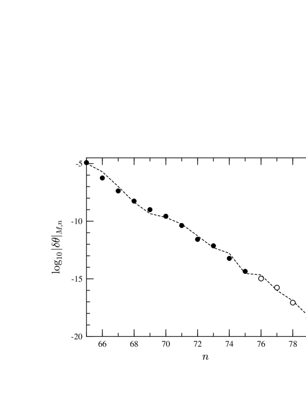
FIG. 14.: Median splittings $|\delta\theta|_{M,n}$ as a function of angular momentum (logarithmic plot). Exact splittings are obtained from numerical diagonalization (full circles), calculation of $|[S^{N}]_{n,-n}|$ for large $N$ (empty circles), and estimates are taken from the median formula (80) and corrected by $c=1/6$ (dashed line).

Fig. 14 depicts the median values of eigenphase splittings of doublets peaked at angular momenta $n=65,\ldots,80$ as a function of $n$. Full circles represent median splittings $|\delta\theta|_{M,n}$ as obtained from numerical diagonalization. Since the diagonalization routine cannot differentiate between eigenvalues which are closer than $\sim 10^{-15}$, splittings beyond $n=75$ could not be resolved directly. Instead, they were extracted by use of Eq. (30), that is, by numerical calculation of $2[S^{N}]_{n,-n}/N$ for large $N\lesssim|\delta\theta_{n}|^{-1}$. Empty circles represent median splittings thus obtained from $30$ configurations with $R$ ranging from $R=1$ to $R=1.3$. We have taken the edge region to extend over angular momenta $\ell=56,\ldots,64$ and have chosen $\ell_{\text{COE}}=50$. To account for the over-estimate of the splitting by Eq. (80), theoretical predictions are multiplied by an overall factor $c\approx 1/6$. The dashed line shows the resulting approximation for the median splittings. Apart from the factor $c$, the formula (80) is in good agreement with the exact median splittings.

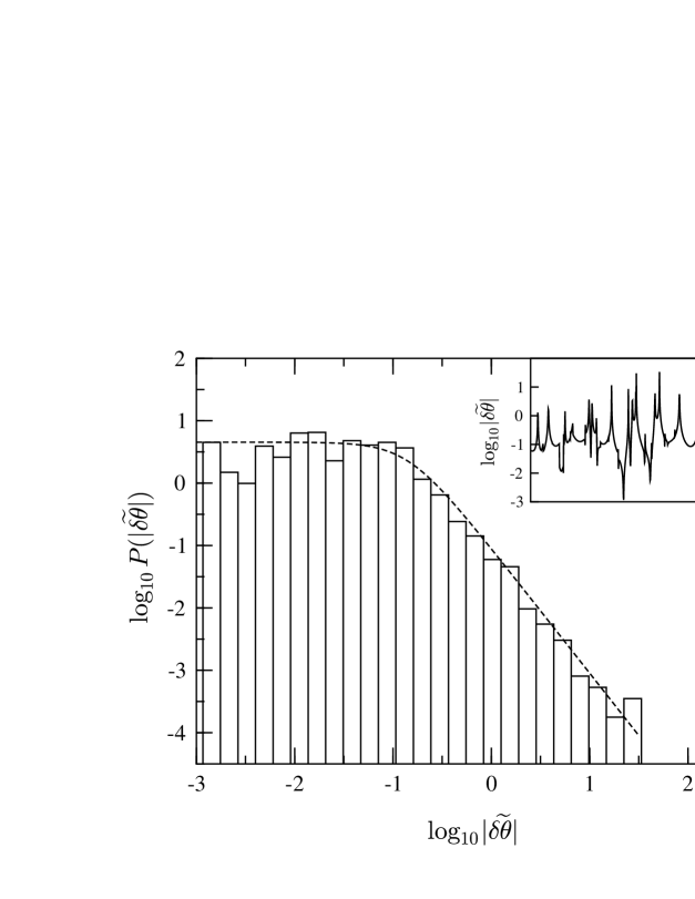
FIG. 15.: Distribution function $P(|\widetilde{\delta\theta}|)$ for the “reduced” splitting $|\widetilde{\delta\theta}|$ (solid line), compared to the predicted Cauchy distribution (dashed line), double logarithmic plot. Inset: “reduced” splittings obtained after unfolding the modulations due to the beach layers.

Let us turn to the splitting statistics. If one is interested in the fluctuations due to changes in the chaotic dynamics, one first has to discard the slow modulation due to the change of beach layer properties. We do so by considering the “reduced” splitting $\widetilde{\delta\theta}_{n}$ of Eq. (53) for those values of $R$ at which one single $\ell$ is dominant in both shift and splitting (for $n=65,\ldots,67$, and here $\ell=n-7$). We find that the median of $\widetilde{\delta\theta}_{n}$ is approximately equal to $c$, independent of $n$ (not shown). Fig. 15 confirms that the distribution $P(|\widetilde{\delta\theta}|)$ falls off like a Cauchy distribution of width $c$. For the figure, 750 exact splittings were transformed to reduced ones (see inset) and collected in a histogram with log-binning (main figure, solid line). This is compared to the Cauchy distribution $2c\pi^{-1}/(c^{2}+\widetilde{\delta\theta}{}^{\,2})$ (main figure, dashed line). The agreement is very good.

Finally, we show in Fig. 16 the distribution function $P(|\delta\theta_{n}|/|\delta\theta|_{M,n}\!)$ of exact splittings divided by the median splittings displayed in Fig. 14. The actual splittings display a power law $P(|\delta\theta|)\sim|\delta\theta|^{-3/2}$ (dashed line). This can be understood by realizing that the variation in $R$ is sufficiently large to average not only over avoided crossings between chaotic and regular eigenphases, but also over avoided crossings between regular and beach eigenphases. These avoided crossings, however, appear in the sum (42) with a squared phase denominator $d_{n,\ell}^{-2}$, and we have argued in Eq. (73) that the distribution generated by such contributions displays a power-law decay with exponent $-3/2$. The exponent $-3/2$ conforms to the findings of Leyvraz and Ullmo [10], who studied chaos-assisted tunneling in the presence of a imperfect transport barrier in the chaotic sea.

FIG. 16.: Distribution of original eigenphase splittings $|\delta\theta_{n}|$, for each $n$ divided by the median $|\delta\theta|_{M,n}$ (solid line), double logarithmic plot. Dashed line: comparison to a $\delta\theta^{-3/2}$ power-law decay, prefactor fitted to the data.

VI Discussion

A Possible Experimental Realizations

Even though the occurrence of chaos-assisted tunneling should be a very general phenomenon, an experimental proof of the effect has not yet been given. The main difficulty might not be to measure the effect, but to recognize it. As long as little is known about tunneling in multi-dimensional mixed systems in general, it will be difficult to separate out the different contributions to the tunneling rates and to identify the effects of classical transport. It is our strong suspicion that, as soon as qualitative theories for experimental systems are developed, chaos-assisted tunneling will turn out to be a frequent effect in the splitting of dynamical tunneling doublets.

1 Superconducting Microwave Cavities

It has been argued in this work that the annular billiard serves as an excellent paradigm for chaos-assisted tunneling. An experimental realization of it is presently investigated by the Darmstadt group of Richter et al. [47]. Performing resonance measurements on a superconducting niobium microwave cavity, the Darmstadt group has extracted high-quality spectra in the frequency range 0–20 GHz, corresponding to $k=0$–50 in our units, but experimental accuracy does not yet allow a resolution of the splittings of high-angular momentum doublets. However, it might be just as interesting to measure the energy splittings of beach doublets, as these splittings are also chaos-assisted, but by orders of magnitudes larger than those of the regular doublets.

2 Atomic Systems

Atomic systems have served as paradigms of many predictions in quantum chaos, and there are some atoms in which an observation of chaos-assisted tunneling might be conceivable. Hydrogen in a weak magnetic field [48] may be such a case. In the weak field limit, the classical system has symmetry-connected regular islands corresponding to low-angular momentum motion along the field axis on either side of the hydrogen core. These islands are separated by a chaotic sea, and dynamical tunneling between the corresponding low-angular momentum quantum states should therefore be enhanced by chaos-assisted processes. It is however not clear, whether these splittings are large enough to be experimentally accessible. Another much-studied system in the field of quantum chaos, the quantum kicked rotor, has recently been experimentally realized by Moore et al. [49] using ultracold sodium atoms in pulsed, near-resonant light. Rotor systems have been considered by several groups in studies of dynamical tunneling in the presence of chaos [22, 50], and a link between theory and experiment might soon become possible. Again, the experiment might still be far from the required degree of accuracy.

3 Open Systems

Finally, chaos-assisted processes can enhance not only tunneling oscillations, but also the decay of regular modes in a mixed, open system in which the dominant coupling to the continuum is mediated by states residing on the chaotic layer. Experimental realizations of such systems were studied by Nöckel et al. and others [51] who considered the $Q$-spoiling of whispering gallery modes in deformed lasing droplets. In a recent work, Hackenbroich and Nöckel [52] also considered mixed systems in which the direct coupling of regular modes to the continuum is suppressed, but where chaotic states have sizable coupling to the continuum. Regular modes may then decay via a multi-step process of type regular-chaotic-continuum. Their results were motivated by a study of a modified version of the annular billiard, in which the outer circle is replaced by a mirror, and the billiard is supposed to have higher optical density that the exterior region outside the mirror. It was found that chaos-assisted decay can lead a dramatic enhancement of level widths.

B Discussion and Conclusions

Having discussed the experimental perspectives, one is immediately led to the question of the general applicability of the method and the block-matrix model proposed in this work.

It is clear that the scattering problem must be solved separately for each system under consideration. In a general system, it might be very difficult to formulate the $S$-matrix and to find a basis in which the $S$-matrix elements $S_{n,n}$ and $S_{-n,-n}$ corresponding to motion on the tunneling tori are sufficiently close to unity. It must however be said in favor of the scattering approach that the difficulty of finding an EBK-quantization scheme in non-separable systems is by no means inherent to the scattering approach, but presently poses one of the most serious problems of semiclassical theory in general [53]. (In fact, it is one of the fortunate aspects of the annular billiard that the angular momentum basis is semiclassically diagonal in the region of regular motion.)

In situations where $S_{\pm n,\pm n}$ are not sufficiently close to unity, Eqs. (21,22) may still work well, provided that sufficient knowledge of eigenvector structure is available (see [36] for an application to the case of rough billiards [54] and other systems). However, calculation of the splitting by summation over long paths from $n$ to $-n$ relies on a sufficient localization of $|\mathchoice{{\hbox{\boldmath$\displaystyle n$}}}{{\hbox{\boldmath$\textstyle n$}}}{{\hbox{\boldmath$\scriptstyle n$}}}{{\hbox{\boldmath$\scriptscriptstyle n$}}}\rangle$ at the $n$-th component.

Clearly, the block matrix model used in the summation over paths must be adopted to the specific transport situation encountered. In case of structure other than the beach layers, additional blocks must be introduced. This does however not lead to problems in the summation Eq. (38) as long as the outermost tunneling element is smaller than any of the internal coupling elements. At present, there is no a priori method to determine the border indices of neighboring blocks inside the chaotic layer. However, use of classical information will warrant correct results to within an order of magnitude.

We note that our treatment is not limited to the case of an $S$-matrix symmetry $S_{n,m}=S_{-n,-m}$ and could easily be extended to non-symmetric systems (for example, an annular billiard with the inner circle replaced by some non-symmetric shape), or even to the case of tunneling at an accidental degeneracy between two eigenphases. In the summation over paths, we merely require that the initial and the final diagonal $S$-matrix elements are equal, $S_{n_{i},n_{i}}=S_{n_{f},n_{f}}$. Note, however, that in the non-symmetric case the contributions $\langle\mathchoice{{\hbox{\boldmath$\displaystyle n$}}}{{\hbox{\boldmath$\textstyle n$}}}{{\hbox{\boldmath$\scriptstyle n$}}}{{\hbox{\boldmath$\scriptscriptstyle n$}}}_{i}|S^{N}|\mathchoice{{\hbox{\boldmath$\displaystyle n$}}}{{\hbox{\boldmath$\textstyle n$}}}{{\hbox{\boldmath$\scriptstyle n$}}}{{\hbox{\boldmath$\scriptscriptstyle n$}}}_{i}\rangle$ and $\langle\mathchoice{{\hbox{\boldmath$\displaystyle n$}}}{{\hbox{\boldmath$\textstyle n$}}}{{\hbox{\boldmath$\scriptstyle n$}}}{{\hbox{\boldmath$\scriptscriptstyle n$}}}_{f}|S^{N}|\mathchoice{{\hbox{\boldmath$\displaystyle n$}}}{{\hbox{\boldmath$\textstyle n$}}}{{\hbox{\boldmath$\scriptstyle n$}}}{{\hbox{\boldmath$\scriptscriptstyle n$}}}_{f}\rangle$ in Eq. (19) will in general not cancel. Their difference is then likely to dominate the splitting.

It is one of our main results to point out the importance of the beach layer to the chaos-assisted tunneling phenomenon. The appearance of classically chaotic, but not too unstable regions around regular islands is generic in mixed systems. Such regions should always support states if the mixing with the rest of phase space is sufficiently slow (or if energy is sufficiently low). However, it must be checked whether some of the importance of the beach layer should actually be attributed to the tunneling ridge that favors tunneling processes into the beach region (see Fig. 5). Such a test is given in our version of the Bohigas numerical experiment, see Section IV F. We have verified that, at small $\delta$, there are no visible tunneling ridges, and the tunneling amplitudes decay monotonically away from the diagonal. Nevertheless the beach region still governs the behavior of the eigenphase splittings (see Fig. 11). It must however be noted that, in this case, the correspondence between slow splitting modulations and the shift breaks down. The shift is then determined by paths $n\rightarrow n-1\rightarrow n$ instead of paths leading to the beach and back to $n$.

It is another interesting point that the statistical results found in Section V are independent of the explicit joint distribution function of eigenphases, but can be derived under rather general assumptions. We merely require that the joint distribution of eigenphases vanishes at eigenphase degeneracies.

This generality is extended even further by the observation that enhancement of tunneling can also appear with help of regular states. Indeed, in Section IV F we have even observed the case of tunneling between a chaotic doublet via a resonant regular state. This should serve as a reminder that only the phase space topology determines the occurrence of tunneling, not its regularity or chaoticity, and that chaos-assisted tunneling is, in fact, a more general phenomenon of transport-assisted tunneling. Additionally, the tunneling rate seems to be rather insensitive to the rate of classical flux connecting the opposite beach regions — as long as there exists a classically allowed path between them. When changing $\delta$ in Section IV F, most of the tunneling enhancement was related to the change of tunneling properties between the torus and the beach region. Progressively rapid classical propagation across the chaotic layer was related to tunneling enhancement of only one order of magnitude — out of five orders of magnitude in total ($\delta=0.07$–0.15).

Our study of chaos-assisted tunneling has led to the most quantitative treatment of the phenomenon to date. At the same time, some challenging problems have been encountered. For example, we have seen that tunneling can occur between doublets localized on “soft” phase space structures such as the beach regions or scarring periodic orbits. For these states, transport from one phase space structure to its symmetry-related partner is classically allowed, but quantum mechanically forbidden. Apart from the intriguing question about the quantum-mechanical localization mechanism giving rise to these states, their doublet structure introduces additional complications. For example, some of the doublets tunnel via resonant processes, while others tunnel directly. A quantitative treatment would certainly be desirable.

C Summary

We studied dynamical tunneling between symmetry-related phase space tori that are separated by a chaotic region. Using scattering theory, we introduced a unitary matrix $S$ that constitutes the quantum analogue of the classical Poincaré map. By expressing eigenphase splittings and shifts in terms of matrix elements of high iterates of $S$, we related these quantities to paths in phase space. While paths contributing to the splitting connect the two tunneling tori, paths that contribute to the shift lead from a tunneling torus back to itself, leaving the torus at least once. We performed the summation over paths within a block-matrix approximation, allocating different blocks to the two regular regions, the chaotic sea, and the two intervening beach layers. Within this approximation, we derived analytic expressions for the contributions to the tunneling properties. Explicit inclusion of the beach blocks enabled us to predict a number of new effects that could be verified for the case of the annular billiard. (I) As a function of an external parameter the splitting varies on two scales: a rapid one attributed to resonance denominators of regular and chaotic states, and a slow one attributed to (squared) resonance denominators between regular states and beach states. This diversity of scales is also observed in statistical quantities, e.g the distribution function $P(\delta\theta)$ of eigenphase splittings $\delta\theta$. When averaging over a sufficiently small range of a system parameter (such that beach properties remain effectively constant), the splittings are distributed with a Cauchy tail $P(\delta\theta)\sim\delta\theta^{-2}$. When averaging over a large parameter range (such that beach resonances occur), the squared resonance denominators lead to a $P(\delta\theta)\sim\delta\theta^{-3/2}$ power-law behavior. (II) Typically, the shift varies on the slow scale only and is much larger than the splitting.

Analytical formulas at hand, we could also asses the relative importance of tunneling amplitudes and classical transport properties within the chaotic sea. As the annular billiard’s eccentricity is increased, most of the enhancement of tunneling rates can be attributed to the tunneling amplitudes and resonances between regular tori and the beach regions. Progressively faster classical transport within the chaotic sea was found to play a minor role in the splitting enhancement.

Finally, we derived the asymptotic form $P(\delta\theta)\sim\delta\theta^{-2}$ of the splitting distribution’s large-$\delta\theta$ tail (average over a small parameter range). In this calculation, no explicit assumption about the form of the joint distribution function of chaotic eigenphases was made; it was merely required that the distribution is either Poissonian or vanishes for degenerate eigenphases. In order to give “typical” splitting values, we calculated the median splitting by averaging over the properties of the chaotic sea. Apart from an over-estimate by an overall factor $\sim 5$, the predicted values for the median splittings closely follow the numerical results over many orders of magnitude.

It is a pleasure to thank H. A. Weidenmüller for many conversations and support. Also, we thank O. Bohigas, F. von Oppen, S. Tomsovic, and D. Ullmo for discussions on several occasions. This work was partially funded by a grant from MINERVA.

A Summation over Paths in the Splitting Formulas

In this Appendix we will derive formula (38) that contains the contributions of the different families of paths to the full sum over paths

$\displaystyle{\cal P}^{N}_{n,-n}={\sum_{\{n\>\rightarrow-n\}}}\prod_{i=1}^{N-1}\>S_{\lambda_{i},\lambda_{i+1}}$

leading from $n$ to $-n$. Recall that ${\cal P}^{N}_{n,-n}$ is related to the splitting of the doublet $\delta\theta_{n}^{\pm}$ by Eq. (32). As $N\sim\kappa/\delta\theta_{n}$ is taken to be large, we need only collect the leading-order contribution in $N$.

Let us consider the general case in which the $S$-matrix and block-diagonalized into any number of blocks $S^{(i,j)}$, $i,j=0,\ldots,K$. For the summation over paths, we merely require that the outermost couplings $S_{\lambda,\lambda^{\prime}}^{(0,j)}$ and $S_{\lambda,\lambda^{\prime}}^{(j,K)}$ be much smaller than entries of the internal coupling matrices. Suppose we want to collect the contributions from paths with $M+1$ steps that start from $n$ and pass through the $M$ intermediate diagonal blocks $S^{(i_{1},i_{1})},S^{(i_{2},i_{2})},\ldots,S^{(i_{M},i_{M})}$ before arriving at $-n$, and let us for the moment neglect repetitions in the block indices. It is equivalent to sum over all such paths in the block-tridiagonal matrix

$$\left(\begin{array}[]{cccccc}D_{0}&C_{0}^{\prime}&&&&\\ C_{0}&D_{1}&C_{1}^{\prime}&&0&\\ &C_{1}&D_{2}&\ddots&&\\ &&\ddots&\ddots&C_{M-1}^{\prime}&\\ &0&&C_{M-1}&D_{M}&C_{M}^{\prime}\\ &&&&C_{M}&D_{0}\end{array}\right)\ ,$$ (A7)

where each of the diagonal blocks $D_{i}=S_{\lambda,\lambda}^{(i,i)}\delta_{\lambda,\lambda^{\prime}}$ is coupled to its neighbor by the coupling block $C_{i}=S_{\lambda,\lambda^{\prime}}^{(i,i+1)}$. $C^{\prime}$ is a short notation for the other coupling block, $C_{i}^{\prime}=S_{\lambda^{\prime},\lambda}^{(i+1,i)}$ (which need however not be the transpose of $C_{i}$, as $S$ is in general not symmetric). $D_{0}=S_{n,n}=S_{-n,-n}$ contains the diagonal $S$-matrix element associated with the tunneling tori.

In addition to summations over the matrix indices of each block, we have to sum over the staying times $N_{0},\ldots,N_{M}$ inside the diagonal blocks $D_{0},\ldots,D_{M}$, respectively. Explicitly, we have to perform the sum

$$\sum_{\{N_{0},\cdots N_{M}\}}\!\!D_{0}^{\,N_{0}}\,C_{0}\,D_{1}^{\,N_{1}}\cdots D_{M}^{N_{M}}\,C_{M}\,D_{0}^{\,N-N_{0}-N_{1}\ldots-N_{M}-M}$$ (A8)

$$=\>D_{0}^{\,(N-M)}\!\!\sum_{\{N_{0},\cdots N_{M}\}}\!\!C_{0}\,(D_{1}/D_{0})^{N_{1}}\cdots(D_{M}/D_{0})^{N_{M}}\,C_{M}\ ,$$ (A9)

where the summations go over $N_{M}=0,\ldots,N-M$, $N_{M-1}=0,\ldots,N-N_{M}-M$, and so on, up to $N_{0}=N-N_{M}-N_{M-1}-\ldots-N_{1}-M$. Summing over $N_{0}$ is trivial and generates a factor $(N-N_{M}-\ldots-N_{1}-M+1)$. The remaining sums are then performed by repeated use of the formula

$$\sum_{\rho=0}^{R}(R-\rho+1)\,z^{\rho}=\frac{R+2}{1-z}+\frac{z^{R+2}-1}{(1-z)^{2}}\ ,$$ (A10)

For $z=D_{i}/D_{0}$ of absolute value $|z|<1$, we need only keep the term $R/(1-z)$, because in further summations the remaining terms generate sub-dominant contributions of ${\cal O}(1)$ or ${\cal O}(|z|^{N})$. Neglecting these terms is justified in our case, because we have assumed that the outermost (tunneling) matrix elements are much smaller than internal transition elements and by unitarity, $|D_{i}|<|D_{0}|$ for all $i\neq 0$. Keeping only the term $R/(1-z)$ of (A10), the structure of the sum always remains the same, and each summation results in a multiplicative factor $(1-D_{i}/D_{0})^{-1}$. We arrive at the result that the sum over paths of length $M$ passing through the blocks $D_{0},\ldots,D_{M}$ is given as

$${\cal P}_{n,-n}^{N\,(i_{1},\ldots,i_{M})}\sim N\>D_{0}^{\,(N-1)}\>C_{0}\>\prod_{i=1}^{M}\>\left[\>\frac{1}{D_{0}-D_{i}}\,C_{i}\>\right]\ .$$ (A11)

Eq. (A11) was formulated without allowing for repetitions in block indices and contains all coupling elements to lowest order. Loops in block index space that stay within the inner blocks can however be included by allowing repeated indices in Eq. (A11). Paths with $k$ repetitions of the index combination $(i,i+1)$, say, then give rise to contributions containing a factor $[(D_{0}-D_{i})^{-1}C_{i}^{\prime}(D_{0}-D_{i+1})^{-1}C_{i}]^{k}$. The number of repetitions can be summed over, which leads to an expression as in Eq. (A11) with the replacement

$$\frac{1}{D_{0}-D_{i}}\>C_{i}\quad\mapsto\quad$$ (A12)

$$\frac{1}{D_{0}-D_{i}}\>C_{i}\;\left[1-\frac{1}{D_{0}-D_{i+1}}\>C_{i}^{\prime}\>\frac{1}{D_{0}-D_{i}}\>C_{i}\right]^{-1}\ .$$ (A13)

All types of loops can be included by the corresponding replacements, giving rise to a continued fraction structure of ${\cal P}_{n,-n}^{N\,(i_{1},\ldots,i_{M})}$.

REFERENCES

- [1] Permanent address: Mathematics-Physics Department, University of Haifa at Oranim, Tivon 36006, Israel.
- [2] O. Bohigas, S. Tomsovic, and D. Ullmo, Phys. Rev. Lett. 65, 5 (1990).
- [3] A. Einstein, Verhandl. deut. physik. Ges. 19, 82 (1917); L. Brillouin, J. phys. radium 7, 353 (1926); J. B. Keller, Ann. Phys. (New York) 4, 180 (1958).
- [4] M. C. Gutzwiller, Chaos in Classical and Quantum Mechanics (Springer–Verlag, New York, 1990).
- [5] W. A. Lin and L. E. Ballentine, Phys. Rev. Lett. 65, 2927 (1990); Phys. Rev. A 45, 3637 (1992); A. Peres, Phys. Rev. Lett. 67, 158 (1991).
- [6] O. Bohigas, S. Tomsovic, and D. Ullmo, Phys. Rep. 223, 43 (1993).
- [7] R. Utermann, T. Dittrich, and P. Hänggi, Phys. Rev. E 49, 273 (1994).
- [8] O. Bohigas, D. Boosé, R. Egydio de Carvallho, and V. Marvulle, Nucl. Phys. A 560, 197 (1993).
- [9] S. Tomsovic and D. Ullmo, Phys. Rev. E 50, 145 (1994).
- [10] F. Leyvraz and D. Ullmo, J. Phys. A 10, 2529 (1996).
- [11] E. Doron and S. D. Frischat, Phys. Rev. Lett. 75, 3661 (1995).
- [12] A. J. Lichtenberg and M. A. Lieberman, Regular and Stochastic Motion (Springer, New York, 1983).
- [13] E. P. Wigner, Phys. Rev. 40, 749 (1932); M. Hillery, R. F. O’Connell, M. O. Scully, and E. P. Wigner, Phys. Rep. 106, 121 (1984).
- [14] K. Husimi, Proc. Phys. Math. Soc. Jpn. 22, 264 (1940); K. Takahashi, Prog. Theo. Phys. Suppl. 98, 109 (1989).
- [15] E. J. Heller, Phys. Rev. Lett. 53, 1515 (1984).
- [16] D. W. Noid and R. A. Marcus, J. Chem. Phys. 67, 559 (1977).
- [17] O. Bohigas, S. Tomsovic, and D. Ullmo, Phys. Rev. Lett. 64, 1479 (1990).
- [18] V. P. Maslov, The Perturbation Series and Asymptotic Methods (Moscow University, Moscow, 1965).
- [19] W. H. Miller and T. F. George, J. Chem. Phys. 56, 5668 (1972); Adv. Chem. Phys. 25, 69 (1974).
- [20] W. H. Miller, Adv. Chem. Phys. 30, 77 (1975).
- [21] M. J. Davis and E. J. Heller, J. Chem. Phys. 75, 246 (1981).
- [22] G. Casati, R. Graham, I. Guarneri, and F. M. Izrailev, Phys. Lett. A 190, 159 (1994).
- [23] S. D. Frischat and E. Doron, J. Phys. A 30, 3613 (1997).
- [24] M. Wilkinson, Physica 21D, 341 (1986); M. Wilkinson, J. Phys. A 20, 635 (1987); S. C. Creagh and N. D. Whelan, Phys. Rev. Lett. 77, 4975 (1996).
- [25] O. Bohigas, in Proceedings of the 1989 Les Houches Summer School on “Chaos and Quantum Physics”, edited by M.-J. Giannoni, A. Voros, and J. Zinn-Justin (Elsevier Science Publishers B.V., Amsterdam, 1991), p. 547.
- [26] A. Richter, Playing Billiard with Microwaves (to appear in Proceedings of the Workshop on “Emerging Applications of Number Theory” University of Minnesota, Minneapolis, 1996).
- [27] E. Doron and U. Smilansky, Nonlinearity 5, 1055 (1992).
- [28] E. B. Bogomolny, Nonlinearity 5, 805 (1992).
- [29] R. Blümel and U. Smilansky, Phys. Rev. Lett. 64, 241 (1990).
- [30] M. Abramowitz and I. A. Stegun, Handbook of Mathematical Functions (Dover Publications, New York, 1964).
- [31] M. V. Berry and K. E. Mount, Rev. Prog. Phys. 35, 315 (1972).
- [32] S. D. Frischat, Ph.D. thesis, Heidelberg University, 1996.
- [33] E. Doron and S. D. Frischat, (unpublished).
- [34] W. Franz, Z. Naturforschg. 9, 705 (1954).
- [35] J. B. Keller, J. Opt. Soc. Am. 52, 116 (1962).
- [36] G. Hackenbroich, E. Narimanov, and A. D. Stone, Quantum Perturbation Theory for the Level Splitting in Billiards, (preprint, May 1997).
- [37] R. S. MacKay, J. D. Meiss, and I. C. Percival, Phys. Rev. Lett. 52, 697 (1984); Physica D 13, 55 (1984).
- [38] R. T. Swimm and J. B. Delos, J. Chem. Phys. 71, 1706 (1979).
- [39] O. Bohigas, M. J. Giannoni, and C. Schmit, Phys. Rev. Lett. 52, 1 (1984).
- [40] R. Blümel and U. Smilansky, Phys. Rev. Lett. 60, 477 (1988).
- [41] F. J. Dyson, J. Math. Phys. 3, 140 (1962).
- [42] P. Gerwinsiki and P. Šeba, Phys. Rev. E 50, 3615 (1994).
- [43] D. Klakow and U. Smilansky, J. Phys. A 29, 3213 (1996).
- [44] H. P. Baltes and E. R. Hilf, Spectra of Finite Systems (BI Wissenschaftsverlag, Mannheim, 1978).
- [45] I. S. Gradshteyn and I. M. Ryzhik, Table of Integrals, Series and Products (Academic Press, San Diego, 1965).
- [46] We thank Felix von Oppen for contributing the main idea for this calculation.
- [47] R. Hofferbert, Untersuchung von wellendynamischem Chaos in supraleitenden Mikrowellen-Billards, master thesis, Technische Hochschule Darmstadt, 1994.
- [48] H. Friedrich and D. Wintgen, Phys. Rep. 183, 37 (1989); D. Delande, in Proceedings of the 1989 Les Houches Summer School on “Chaos and Quantum Physics”, edited by M.-J. Giannoni, A. Voros, and J. Zinn-Justin (Elsevier Science Publishers B.V., Amsterdam, 1991), p. 665.
- [49] F. L. Moore et al., Phys. Rev. Lett. 75, 4598 (1995).
- [50] V. Averbukh, N. Moiseyev, B. Mirbach, and H. J. Korsch, Z. Phys. D 35, 247 (1995).
- [51] J. U. Nöckel, A. D. Stone, and R. K. Chang, Opt. Lett. 19, 1693 (1994); A. Mekis et al., Phys. Rev. Lett. 75, 2682 (1995); J. U. Nöckel and A. D. Stone, Nature 385, 45 (1997).
- [52] G. Hackenbroich and J. U. Nöckel, Chaos-assisted tunneling in open systems, (preprint, June 1996).
- [53] S. Tomsovic, M. Grinberg, and D. Ullmo, Phys. Rev. Lett. 75, 4346 (1995); D. Ullmo, M. Grinberg, and S. Tomosovic, Phys. Rev. E 54, 136 (1996).
- [54] K. M. Frahm and D. L. Shepelyansky, Phys. Rev. Lett. 78, 1440 (1997).