Algebraic approximations to bifurcation curves of limit cycles for the Liénard equation
Hector Giacomini and Sébastien Neukirch
Laboratoire de Mathématiques et Physique Théorique
C.N.R.S. UPRES A6083
Faculté des Sciences et Techniques, Université de Tours
F-37200 Tours FRANCE

Abstract

In this paper, we study the bifurcation of limit cycles in Liénard systems of the form $\frac{dx}{dt}=y-F(x)\quad,\quad\frac{dy}{dt}=-x$ , where $F(x)$ is an odd polynomial that contains, in general, several free parameters. By using a method introduced in a previous paper, we obtain a sequence of algebraic approximations to the bifurcation sets, in the parameter space. Each algebraic approximation represents an exact lower bound to the bifurcation set. This sequence seems to converge to the exact bifurcation set of the system. The method is non perturbative. It is not necessary to have a small or a large parameter in order to obtain these results.

PACS numbers : 05.45.+b , 02.30.Hq , 02.60.Lj , 03.20.+i

Key words : Bifurcation, Liénard equation, limit cycles. The Liénard equation [1] :

$$\frac{d^{2}x}{dt^{2}}+f(x)\frac{dx}{dt}+x=0$$ (1)

appears very often within several branches of science, such as physics, chemistry, electronics, biology, etc (see [2, 3] and references therein).

This equation can be written as a two-dimensional dynamical system which reads as follows :

$$\frac{dx}{dt}=y-F(x)\quad,\quad\frac{dy}{dt}=-x$$ (2)

where $F(x)=\int_{0}^{x}f(\tau)d\tau$.
The most difficult problem connected with the study of equation (2) is the question of the number and location of limit cycles.

In order to make progress with this problem, it is of fundamental importance to control the bifurcations of limit cycles that can take place when one or several parameters of the system are varied. The word bifurcation is used to describe any sudden change that occurs while parameters are being smoothly varied in any dynamical system. Connections with the theory of bifurcations penetrate all natural phenomena. The differential equations describing real physical systems always contain parameters whose exact values are, as a rule, unknown. If an equation modeling a physical system is structurally instable, that is if the behavior of its solutions may change qualitatively through arbitrary small changes in its right-hand side, then it is necessary to understand which bifurcations of its phase portrait may occur through changes of the parameters.

In this respect, the most difficult bifurcation is the so-called saddle-node bifurcation of limit cycles : let us suppose that system (2) depends on a parameter $\lambda$ : $F=F(x,\lambda)$. Let $\Gamma_{0}$ be a non-hyperbolic limit cycle of (2) (see [9] for a definition) , corresponding to the value $\lambda_{0}$ of the parameter $\lambda$. System (2) undergoes a saddle-node bifurcation at $\lambda=\lambda_{0}$ if for $\lambda=\lambda_{0}+\epsilon$ and $\epsilon$ positive and sufficiently small, the limit cycle $\Gamma_{0}$ bifurcates into two hyperbolic limit cycles, one stable and the other instable. Moreover, for $\lambda=\lambda_{0}-\epsilon$, the limit cycle $\Gamma_{0}$ disappears and there is no limit cycle in a small neighborhood of $\Gamma_{0}$. This bifurcation is particularly difficult to detect because for $\lambda=\lambda_{0}-\epsilon$ there is no trace of it. Moreover, the value of $\lambda_{0}$ is not known in principle and it is not possible to employ a perturbative method with respect to $\epsilon$ to study this type of bifurcation.

In a previous paper [3], we have introduced a method for studying the number and location of limit cycles of (2), for the case where $F(x)$ is an odd polynomial of arbitrary degree. The method is as follows : we consider a function $h_{n}(x,y)$ given by :

$$h_{n}(x,y)=y^{n}+g_{n-1,n}(x)y^{n-1}+g_{n-2,n}(x)y^{n-2}+...+g_{1,n}(x)y+g_{0,n}(x)$$ (3)

where $g_{j,n}(x)$, with $j=0,1,...,n-1$, are functions of only $x$ and $n$ is an even integer. Then it is always possible to choose the functions $g_{j,n}(x)$ in such a way that :

$$\dot{h}_{n}(x,y)=(y-F(x))\frac{\partial h_{n}}{\partial x}-x\frac{\partial h_{n}}{\partial y}$$

is a function only of the variable $x$ (see also [4]). Then we have :

$$\dot{h}_{n}(x,y)=R_{n}(x)$$ (4)

The functions $g_{j,n}(x)$ and $R_{n}(x)$ determined in this way are polynomials. As explained in [3], if for a given value of $n$, the polynomial $R_{n}(x)$ has no real roots of odd multiplicity, then the system has no limit cycle.

We want to show in this paper that the method presented in [3] enables us to determine algebraic approximations to the bifurcation sets of limit cycles for the Liénard equation. These bifurcation sets can be determined analytically only when the system has a small parameter or a large one (perturbative regime). In the intermediate case (non-perturbative regime), no method is known for determining, in an analytic way, the bifurcation set. We shall show here that our method gives a sequence of algebraic lower bounds to the bifurcation sets. Moreover, this sequence seems to converge to the exact bifurcation set. The method can be applied to any system (2) where $F(x)$ is an odd polynomial.

As an example, we will consider a Rychkov system :

$$F(x)=a_{2}x^{5}+a_{1}x^{3}+a_{0}x$$ (5)

with $a_{2}\neq 0$.
We can take one of the parameters equal to one without loss of generality. Several authors have studied this system with $F(x)$ written as $F(x)=\epsilon(x^{5}-\mu x^{3}+x)$. Rychkov has shown in [5] that this system can have at most two limit cycles and actually has exactly two limit cycles when $\epsilon>0$ and $\mu>2.5$. Rychkov’s results have been improved by Alsholm [6], who lowered the bound of $\mu$ to $2.3178$ and by Odani [7], who obtained an even smaller value $\sqrt{5}$. By a scaling of the variables $x$ and $y$, system (2), with $F(x)$ given by (5), can be written in a more simple form, as follows :

$$F(x)=x^{5}-\mu x^{3}+\delta x$$ (6)

Since there are two parameters, the bifurcation set is given by a curve in the parameter plane $(\mu,\delta)$. Our aim, here, is to obtain information about the bifurcation diagram of the system in this plane.

• For $\delta<0$, thanks to Liénard theorem (see [2]), we know that the system has exactly one limit cycle for arbitrary values of $\mu$.

• For $\delta>0$ and $\mu<0$, the Bendixon criterium (see [2]) enables us to conclude that the system has no limit cycle (the divergence of the vector field, given by $-F^{\prime}(x)$, has a constant sign for all x).

• For $\delta>0$ and $\mu>0$, the system can have two or zero limit cycles , according to Rychkov’s results. In this region of the parameter space there exists a bifurcation curve $B(\mu,\delta)=0$. In the region $B(\mu,\delta)>0$, the system has exactly two limit cycles and for $B(\mu,\delta)<0$, the system has no limit cycle. On the curve $B(\mu,\delta)=0$ the system undergoes a saddle-node bifurcation : there is a unique non-hyperbolic (double) limit cycle.

Obviously, the function $B(\mu,\delta)$ is not known and no analytical method for obtaining this function for arbitrary $\mu$ and $\delta$ exists. We shall obtain a sequence of algebraic approximations to the function $B(\mu,\delta)$.

For a given even value of $n$, let us consider the corresponding polynomial $R_{n}(x)$. The polynomials $R_{n}(x)$ described above, can have, for system (6), one, two or zero positive simple roots, depending on the values of $\mu$ and $\delta$. At least it is the behavior observed for the values of $n$ we considered.

• For $\delta<0$ and $\forall\mu$ , the polynomials $R_{n}(x)$ have one simple positive root.

• For $\mu>0$ and $\delta>0$ , the first quadrant is divided in two regions by a curve $B_{n}(\mu,\delta)=0$. In the region $B_{n}(\mu,\delta)>0$, the polynomial $R_{n}(x)$ has two positive simple roots while in the region $B_{n}(\mu,\delta)<0$ it has no positive root. On the curve $B_{n}(\mu,\delta)=0$, $R_{n}(x)$ has a double positive root.

• For $\mu<0$ and $\delta>0$, the polynomials $R_{n}(x)$ have no real root other than the even-multiplicity root in $x=0$.

It is clear (see [3]) that for $\mu>0$ and $\delta>0$ lying in the region $B_{n}(\mu,\delta)<0$, the system (2) with $F(x)$ given by (6) has no limit cycle. Hence, it is evident that the curve $B_{n}(\mu,\delta)=0$ represents an exact lower bound to the bifurcation curve $B(\mu,\delta)=0$ : the curves $B_{n}(\mu,\delta)=0$ are contained in the region $B(\mu,\delta)<0$ for all even values of $n$.

The functions $B_{n}(\mu,\delta)$ are algebraic and can be determined from the conditions :

$$R_{n}(x)=0\;\;\;\;\mbox{ and }\;\;\;\;\frac{dR_{n}}{dx}(x)=0$$ (7)

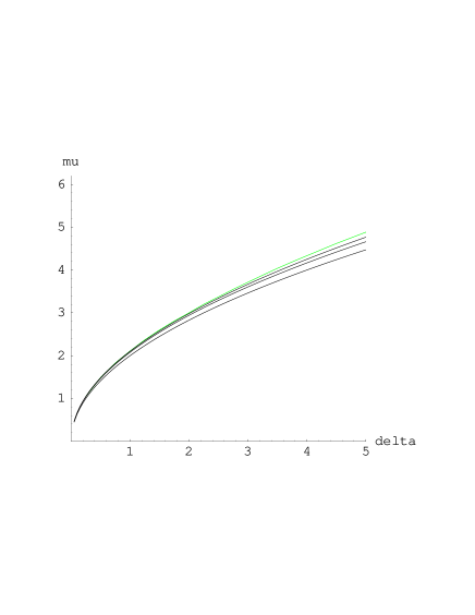
Figure 1: The algebraic curves $B_{n}(\mu,\delta)$ with $n=2,6,14$ (continuous lines) and the bifurcation curve $B(\mu,\delta)$ (dashed line) which is calculated from numerical integrations of system (6).

These two algebraic equations determine the double root of the polynomial $R_{n}(x)$ and give a relation between $\mu$ and $\delta$ which we write $B_{n}(\mu,\delta)=0$. For $n=2$, we find $B_{2}(\mu,\delta)=\delta(\mu^{2}-4\delta)$. For $n=4$, $B_{4}(\mu,\delta)$ is a $12^{th}$ degree polynomial. The degree of $B_{n}(\mu,\delta)$ increases rapidly with $n$. We have calculated the functions $B_{n}(\mu,\delta)$ for even values of $n$ between 2 and 14. The behavior of the curves $B_{n}(\mu,\delta)=0$, as well as the numerical bifurcation curve (calculated from a numerical integration of the system), are shown in fig.(1). We see that each curve $B_{n}(\mu,\delta)=0$ is contained in the region $B_{n-2}(\mu,\delta)>0$. The complete bifurcation diagram is given in fig.(2). There are three regions :

• Region I : There is no limit cycle. All the curves $B_{n}(\mu,\delta)=0$ lie in the part $\mu>0$ of this region.

• Region II : There are two limit cycles. All the polynomials $R_{n}(x,\mu,\delta)$ have two positive simple roots.

• Region III : Liénard theorem shows that there is one limit cycle. All the polynomials $R_{n}(x,\mu,\delta)$ have one positive simple root.

We would like to emphasize that the shape of the bifurcation curve $B(\mu,\delta)=0$ is already given by the curve $B_{2}(\mu,\delta)=\delta(\mu^{2}-4\delta)=0$, which is constructed only with the function $F(x)$ ! The Hopf bifurcation happens when $\delta=0$ and the saddle-node bifurcation occurs near $\mu^{2}=4\delta$.

We shall now make use of this bifurcation curve for the following system :

$$\dot{x} = y-(x^{5}-\frac{\sqrt{5}}{3}(1+\lambda)x^{3}+\lambda x)$$

$$\dot{y} = -x$$ (8)

This example has been studied by Lloyd [8] and Perko [9]. System (8) is a particular case of system (6) with :

$$\mu=\frac{\sqrt{5}}{3}(1+\lambda)\;\;\;\mbox{ and }\;\;\;\delta=\lambda$$

In order to know what are the bifurcations of this system when the $\lambda$ parameter is varied from $-\infty$ to $+\infty$, we must plot the line :

$$\mu=\frac{\sqrt{5}}{3}(1+\delta)$$ (9)

in the bifurcation diagram of system (6), with the exact (but unknown) bifurcation curve $B(\mu,\delta)=0$ replaced by one of the algebraic approximations $B_{n}(\mu,\delta)=0$. As $\lambda$ is varied from $-\infty$ to $+\infty$, the system moves along the line (9) from left to right in fig.(3). It is easy to see that when $\lambda$ is negative (the portion of the line is in region III), there is one limit cycle. Then, when the line crosses the $\mu$ axis (that is when $\lambda$ changes sign) the system undergoes a Hopf bifurcation : a small limit cycle is created around the origin of the phase plane. There are now two limit cycles, the system is in region II. But when $\lambda$ is further increased, the line (9) crosses the bifurcation curve $B(\mu,\delta)=0$ : the two limit cycles collapse in a saddle-node bifurcation and there is no limit cycle , the system is in region I. If we continue to increase $\lambda$, we see the line (9) crossing the curve $B(\mu,\delta)=0$ again : two limit cycles appear in a saddle-node bifurcation, the system enters region II again. We can see that this is the last bifurcation we can create because the line, when $\lambda$ is further increased, does not cross the bifurcation set any more and stays in region II. From the intersections between the line (9) and the curves $B_{n}(\mu,\delta)=0$, we obtain algebraic approximations to the bifurcation values of the parameter $\lambda$.

There is another way to see the different bifurcations of (8). We have claimed in [3] that if $n$ is large enough, the number of positive roots of odd multiplicity of $R_{n}(x)$ gives the number of limit cycles of the system. In the case of system (8), $R_{n}=R_{n}(x,\lambda)$, so when $\lambda$ is varied, the number of roots of $R_{n}$ changes. Hence, for a given value of $\lambda$, the number of limit cycles of (8) can be obtained by counting the number of intersections between the curve $R_{n}(x,\lambda)=0$ and the line $\lambda=\mbox{cte}$ in figure (4).

In [3], we claim that the value of the root of $R_{n}(x)$ gives an approximation to the maximum value of $x$ on the limit cycle (which we call the amplitude). In fig.(4) we have plotted $R_{n}(x,\lambda)=0$ for $n=2\;,n=6$ and $n=10$. So we can see the amplitude of the limit cycles with respect to $\lambda$. We see the Hopf bifurcation when $\lambda$ crosses the x-axis upward and we see the two saddle-node bifurcations when $R_{n}(x,\lambda)$ loses its two positive roots. Once again, as $R_{2}(x,\lambda)=-2xF(x,\lambda)$, an approximation to the bifurcation amplitude-diagram is given by the curve $F(x,\lambda)=0$, which can be written as :

$$\lambda=x^{2}\;\frac{3x^{2}-\sqrt{5}}{\sqrt{5}x^{2}-3}$$

Let’s consider another example :

$$\dot{x} = y-\left(x(x^{2}-a^{2})(x^{2}-2^{2})(x^{2}-5^{2})\right)$$

$$\dot{y} = -x$$ (10)

We want to study the bifurcations of (10), when $a$ is varied from $0\to\infty$. As we already twice noticed, the qualitative bifurcation amplitude-diagram seems to be given by $F(x)=0$. Here, the plot of $F(x,a)=0$ seems to announce the presence of a transcritical bifurcation (see [2] for a definition) near the values $a=2$ and $a=5$ and a Hopf bifurcation for $a=0$ (see fig.(5)). If we plot $R_{4}(x,a)=0$, we still see the Hopf bifurcation, but the supposed-transcritical bifurcations are indeed saddle-node ones (see fig.(6)) : we see that the system can have one or three limit cycles. When $a$ is far from the values $a=2$ or $a=5$, there are three limit cycles, but when $a$ is near the values $a=2$ or $a=5$, there is only one limit cycle. So, in this example, the equation $F(x,a)=0$ does not give the right qualitative amplitude-bifurcation diagram. We must plot the curve $R_{4}(x,a)=0$ in order to obtain the good qualitative shape of it.

In summary, we have introduced a method that gives a sequence of algebraic approximations to the bifurcation sets of limit cycles for the Liénard equation (2). These algebraic approximations are exact lower bounds to the exact bifurcation sets of the system and seem to converge to it in a monotonous way. The fundamental aspect of this method is that it is not perturbative in nature. It is not necessary to have a small or a large parameter in order to apply it.

Acknowledgment : We thanks A. Gassul for bringing reference [4] to our attention after we presented him the results given in [3].

Figure 2: The complete bifurcation diagram of system (2) with $F(x)$ given by (6). On the line $\delta=0$ the system undergoes a Hopf bifurcation. On the curve $B(\mu,\delta)=0$ we have a saddle-node bifurcation of limit cycles. The system has no limit cycle in region I, two limit cycles in region II and one limit cycle in region III.

Figure 3: The line $\mu=\frac{\sqrt{5}}{3}(1+\delta)$ and the bifurcation curve $B(\mu,\delta)=0$ of system (6). The intersections between the two curves give the bifurcation values of $\lambda$ for system (8).

Figure 4: The algebraic approximations to the amplitude-bifurcation diagram for system (8) for the cases $n=2$ (bold), $n=6$ (dash) and $n=10$ (continuous). We see the number and the amplitudes of the limit cycles by considering the intersections between one of these curves and a line $\lambda=\mbox{cte}$. The results are improved with increasing values of $n$.

Figure 5: The curve $F(x,a)=0$ for system (10). We see the number and the amplitude of the limit cycles by considering the intersections between this curve and a line $a=\mbox{cte}$. There seems to be transcritical bifurcations for $a=2$ and $a=5$ at this order.

Figure 6: The curve $R_{4}(x,a)=0$ for system (10). This curve is an approximation to the amplitude-bifurcation diagram. We see the number of limit cycles by counting the number of intersections between this curve and a line $a=\mbox{cte}$. The system only presents saddle-node bifurcations. The qualitative behaviour of the curves $R_{n}(x,a)=0$, with $n>4$, is the same. No further qualitative changes occur for greater values of $n$.

References

- [1] A. Liénard, “Etude des oscillations entretenues”, Rev. Gen. d’électricité, XXIII, 901 (1928).
- [2] S. H. Strogatz, Nonlinear Dynamics and Chaos (Addison Wesley, 1994).
- [3] H. Giacomini and S. Neukirch, “On the number of limit cycles of the Liénard equation”, Physical Review E 56, in press (1997).
- [4] L. A. Cherkas, “Estimation of the number of limit cycles of autonomous systems”, Differential Equations 13, 529 (1977).
- [5] G.S. Rychkov, “The maximal number of limit cycles of the system is equal to two”, Differential Equations 11, 301 (1975).
- [6] P. Alsholm, “Existence of limit cycles for generalized Liénard equations”, J. Math. Anal. Appl. 171, 242 (1992).
- [7] K. Odani, “Existence of exactly N periodic solutions for Liénard systems”, Funkcialaj Ekvacioj 39, 217 (1996) (Japana Matematika Societo).
- [8] N. G. Lloyd, “Liénard systems with several limit cycles”, Math. Proc. Camb. Phil. Soc. 102, 565 (1987).
- [9] L. M. Perko, “Bifurcation of limit cycles : Geometric theory”, Proc. AMS 114, 225 (1992).
- [10] A. Lins, W. de Melo and C. Pugh, On Liénard’s equation, Lecture Notes in Mathematics 597, 335 (1977) (Springer Verlag).