Abstract

The thermodynamic formalism of Ruelle, Sinai, and Bowen, in which chaotic properties of dynamical systems are expressed in terms of a free energy-type function $\psi(\beta)$, is applied to a Lorentz Lattice Gas, as typical for diffusive systems with static disorder. In the limit of large system sizes, the mechanism and effects of localization on large clusters of scatterers in the calculation of $\psi(\beta)$ are elucidated and supported by strong numerical evidence. Moreover it clarifies and illustrates a previous theoretical analysis [1] of this localization phenomenon.

Key words : Lorentz lattice gases, chaos, thermodynamic formalism, Lyapunov exponents, Kolmogorov-Sinai entropy, random walks.

1 Introduction

Many nonlinear physical problems involve a complicated discrete distribution function $\{p_{i}\}$. As it may vary in a very irregular way with $i$, it would be attractive to replace the $p_{i}$’s by a smooth function containing the same information about the structure of the distribution. One way to do it is to associate with the distribution a whole set of so–called “escort distributions” [2] defined as $P_{i}=(p_{i})^{\beta}/Z(\beta)$, where $Z(\beta)$ is a partition function $Z(\beta)\equiv\sum_{i}(p_{i})^{\beta}$. The parameter $\beta$ allows one to scan the structure of the initial distribution. Large $\beta$ values enhance the most probable trajectories whereas negative $\beta$’s focus on the least probable trajectories (we impose that $(p_{i})^{\beta}=0$ if $p_{i}=0$ so that our definitions still hold for negative $\beta$’s). By analogy with thermodynamics where $\beta$ would be an inverse temperature, a free energy—like function $\psi(\beta)$ is introduced, which is related to the logarithm of the dynamic partition function $Z(\beta)$.

This formalism introduced by Ruelle, Sinai and Bowen [3] is called thermodynamic formalism. It has been successfully applied for instance to multifractals [4].

The present paper deals with another frame of application of this formalism, i.e. the chaotic properties of dynamical systems. For a given map (we will assume hyperbolicity in order to ensure good ergodicity properties), the phase space is partitioned into cells. Each sequence of cells explored by a trajectory $(r_{o},\cdots,r_{t})$ in $t$ time steps is one point $\Omega_{t}$ of the dynamical phase space. We shall refer to it as a trajectory over $t$ time steps.

The thermodynamic formalism will be applied to the distribution $P(\Omega_{t})$, where $\Omega_{t}$ replaces the previous subscript $i$. The partition function reads now $Z(\beta,t)=\sum_{\Omega_{t}}P^{\beta}(\Omega_{t})$. Note that each $\Omega_{t}$ is counted with equal weight, i.e. the calculation does not require the a priori knowledge of the invariant measure. The free energy is now defined as $\psi(\beta)=\lim_{t\rightarrow\infty}\frac{1}{t}\ln Z(\beta)$. In this context, it is called Ruelle pressure or topological pressure. It contains information about the dynamics of the system, which can be extracted again by varying the control parameter $\beta$. For example, for an open system, the escape rate $\gamma$ is such that $\psi(1)=-\gamma$, and $\psi(\beta)$ vanishes when $\beta$ is equal to the fractal dimension of the repeller (set of trajectories which never escape).

It has already been found in a more general frame that some non analyticity of the Ruelle pressure may occur at certain $\beta$ values [2, 5, 4]. They are called phase transitions in analogy with thermodynamics.

In this paper, we study the influence of disorder on the structure of the Ruelle pressure. We have applied the thermodynamic formalism to systems with static disorder and have found very peculiar features [6]. In the limit of infinite systems, and for almost all $\beta$ values, the Ruelle pressure becomes completely determined by trajectories localized on rare fluctuations of the disorder. The global structure of the disorder —in particular the density of impurities— becomes irrelevant. Depending on $\beta$, the relevant trajectories are not always localized onto the same type of fluctuations. The crossovers between the different localization regimes are characterized by non-analytical points in the Ruelle pressure.

For finite but large systems, the Ruelle pressure is again analytic. However for most $\beta$’s it is still dominated by localized trajectories. Delocalized trajectories become relevant only in some limited $\beta$ regions which shrink to points as the system size tends to infinity.

To be more precise, we have developed these ideas by studying a particular model, the Lorentz Lattice Gas (LLG). A Lorentz gas consists of a moving light particle scattered among fixed heavy particles. It may be considered as a simple model for diffusion, electric conductivity or flow inside a porous medium. In the past decades, it has been successfully used to study the connection between the irreversible behavior of fluids and their chaotic properties at a microscopic level. For example, P. Gaspard and G. Nicolis [7] have shown that for an open system, the diffusion coefficient can be expressed in terms of the Kolmogorov-Sinai entropy and the sum of the positive Lyapunov exponents for non escaping trajectories. The name Lorentz lattice gas is used when the light particle is, for reasons of simplicity, constrained to move on a (cubic) lattice, with scatterers located at the nodes –or sites.

The localization processes occurring when the thermodynamic formalism is applied to such a system, have already been discussed in an extensive theoretical analysis [1]. The present paper contains the numerical counterpart and demonstrates the validity of our analytical results. It clarifies the mechanism of localization in large systems by explicitly calculating the topological pressure for specific non-random configurations in section 3. In section 4 an exact expression for the Hausdorff dimension of the repeller is obtained for an open LLG. Moreover, numerical studies allow us to find a good estimate for the Ruelle pressure for large but finite systems. As an intermediate result, the distribution for the largest cluster of scatterers in random configurations (section 7) is estimated theoretically, and measured through numerical simulations.

2 Thermodynamic formalism

First we give a more precise definition of our model. A number of $N$ fixed scatterers are randomly placed with a probability $\rho$ on the $L$ sites of a finite one-dimensional lattice ${\mathcal{D}}$, having either periodic or absorbing boundaries. The presence of a scatterer at site $\hbox{\rm\bf r}=\{1,2,\cdots,L\}$ is indicated by the boolean variable $\hat{\rho}(\hbox{\rm\bf r})$, equal to 1 (0) if the site r is occupied (empty), with $\langle\hat{\rho}\rangle=\rho=N/L$.

A light particle, moving on the lattice, is specified at time $t$ ($t=0,1,2,\cdots$) by a state $x_{t}=\{\hbox{\rm\bf r}_{t},\hbox{\rm\bf c}_{it}\}$, where its position r is a site on the lattice and its velocity, $\hbox{\rm\bf c}_{i}=\pm 1$, connects site $\hbox{\rm\bf r}_{t}$ to one of its nearest neighbors. Let $\phi(x,t)=\phi_{i}(\hbox{\rm\bf r},t)$ be the probability to find the moving particle in state $x=\{\hbox{\rm\bf r},\hbox{\rm\bf c}_{i}\}$.

The time evolution of the particle from time $t$ to $t+1$ consists of a possible collision followed by propagation. The collision is defined by the following rules : if there is no scatterer at $\hbox{\rm\bf r}_{t}$, then the particle moves ballistically, i.e. $\hbox{\rm\bf r}_{t+1}=\hbox{\rm\bf r}_{t}+\hbox{\rm\bf c}_{i}$. This is expressed in terms of $\phi_{i}$ as :

$$\phi_{i}(\hbox{\rm\bf r}+\hbox{\rm\bf c}_{i},t+1)=\phi_{i}(\hbox{\rm\bf r},t).$$ (1)

If there is a scatterer at $\hbox{\rm\bf r}_{t}$, i.e. if $\hat{\rho}(\hbox{\rm\bf r}_{t})=1$, then the velocity of the particle is reversed with probability $q$ ($\hbox{\rm\bf c}^{\prime}_{it}=-\hbox{\rm\bf c}_{it}$) or left unchanged with probability $p$ ($\hbox{\rm\bf c}^{\prime}_{it}=\hbox{\rm\bf c}_{it}$), with $p+q=1$. In the propagation step the particle moves over one lattice distance in the direction of its post-collision velocity, i.e. $\hbox{\rm\bf r}_{t+1}=\hbox{\rm\bf r}_{t}+\hbox{\rm\bf c}^{\prime}_{it}$. Then, it hops from one site to the next one in the direction of its velocity $\hbox{\rm\bf c}_{i}$. Again, the corresponding evolution of $\phi_{i}$ is given by :

$$\phi_{i}(\hbox{\rm\bf r}+\hbox{\rm\bf c}_{i},t+1)=a\phi_{i}(\hbox{\rm\bf r},t)+b\phi_{-i}(\hbox{\rm\bf r},t)$$ (2)

with $a=p$ and $b=q=1-p$ (the reason for this notation will become clear later). More generally, we define site dependent transition probabilities

$$\hat{a}(\hbox{\rm\bf r}) = a\hat{\rho}(\hbox{\rm\bf r})+1-\hat{\rho}(\hbox{\rm\bf r})$$

$$\hat{b}(\hbox{\rm\bf r}) = b\hat{\rho}(\hbox{\rm\bf r}).$$ (3)

They depend on the precise configuration of scatterers under consideration.

The probability $\phi(x,t)$ evolves with time according to a Chapman–Kolmogorov (CK) equation with site dependent transition probabilities, obtained by combining equations (1) and (2) :

$$\phi_{i}(\hbox{\rm\bf r}+\hbox{\rm\bf c}_{i},t+1)=\hat{a}(\hbox{\rm\bf r})\phi_{i}(\hbox{\rm\bf r},t)+\hat{b}(\hbox{\rm\bf r})\phi_{-i}(\hbox{\rm\bf r},t),$$ (4)

and more formally

$$\phi(x,t+1)=\sum_{y}w(x|y)\phi(y,t).$$ (5)

The transition matrix $w(x|y)$ represents the probability to go from state $y=\{\hbox{\rm\bf r}^{\prime},\hbox{\rm\bf c}_{j}\}$ to state $x=\{\hbox{\rm\bf r},\hbox{\rm\bf c}_{i}\}$, and is given by

$$w(x|y)=\delta(\hbox{\rm\bf r}-\hbox{\rm\bf c}_{i},\hbox{\rm\bf r}^{\prime})\left[\delta_{ij}\hat{a}(\hbox{\rm\bf r}^{\prime})+\delta_{i,j+1}\hat{b}(\hbox{\rm\bf r}^{\prime})\right].$$ (6)

In the case of absorbing boundaries (open system), boundary states $y=\{\hbox{\rm\bf r}^{\prime},\hbox{\rm\bf c}_{j}\}=\{1,+\}$ and $\{L,-\}$ referring to a particle entering the domain ${\mathcal{D}}$ are excluded from the $y$–summation. This is equivalent to imposing the absorbing boundary conditions (ABC)

$$\phi_{+}(1,t)=\phi_{-}(L,t)=0.$$ (7)

In the case of periodic boundaries (closed system), we impose the periodic boundary conditions (PBC)

$$\phi_{i}(\hbox{\rm\bf r}+L,t)=\phi_{i}(\hbox{\rm\bf r},t).$$ (8)

The transition matrix satisfies the normalization relations

$$\sum_{x}w(x|y)\left\{\begin{array}[]{cc}=1&\mbox{(closed)}\\ \leq 1&\mbox{(open)}.\end{array}\right.$$ (9)

The inequality sign in Eq.(9) for open systems refers to the case where $y=\{\hbox{\rm\bf r},\hbox{\rm\bf c}_{i}\}$ denotes a state at a boundary site r with non–entering velocity (boundary states with entering velocity do not occur). Indeed, the sum over $x$ excludes states where the particle has escaped from the domain ${\mathcal{D}}$. Hence the probability for remaining inside the domain decreases when the particle finds itself on a boundary site.

The special case $\rho=1$ is called a Persistent Random Walk (PRW) where $\hat{a}(\hbox{\rm\bf r})=p$ and $\hat{b}(\hbox{\rm\bf r})=q$ for all r. Then the moving particle simply undergoes a random walk with correlated jumps.

For later analysis it is convenient to also have a different representation of the CK–equation. It can be obtained by eliminating the probabilities $\phi_{i}(\hbox{\rm\bf r},t)$ at non–scattering sites with the help of Eq. (1). Let $r_{k}$ ($k=1,2,\cdots,N$) be the position of the $k$-th scatterer and $R_{k}=r_{k+1}-r_{k}$ the free interval between scatterers. For ABC we define in addition $R_{o}=r_{1}-1$ and $R_{N}=L-r_{N}$. Then it is straightforward to show that the scattering amplitudes $U_{i}(k,t)=\phi_{i}(r_{k},t)$ (probability at scattering site $r_{k}$) satisfy the closed set of equations

$$U_{+}(k+1,t+R_{k}) = aU_{+}(k,t)+bU_{-}(k,t)$$

$$U_{-}(k-1,t+R_{k-1}) = bU_{+}(k,t)+aU_{-}(k,t)$$ (10)

with the boundary conditions

$$U_{i}(N+k,t)=U_{i}(k,t)$$ (PBC) (11)

$$U_{+}(1,t)=U_{-}(N,t)=0 \mbox{(ABC)}.$$

Note that Eq.(10) only depends on the set of random intervals $\{R_{k}\;|\;k=0,1,2,\cdots,N\}$ (the coefficients $a=p$ and $b=q$ are sure variables), whereas the CK-equation (4) depends on the set of random transition rates $\{\hat{a}(\hbox{\rm\bf r}),\hat{b}(\hbox{\rm\bf r})\;|\;\hbox{\rm\bf r}=1,2,\cdots,L\}$. It will appear below that the basic chaos properties can be expressed in terms of the largest eigenvalue $\Lambda$ and the corresponding left and right eigenvectors $v(x)=v_{i}(\hbox{\rm\bf r})$ and $u(x)=u_{i}(\hbox{\rm\bf r})$ of the non-symmetric matrix $w$ appearing in the CK–equation (5) :

$$wu = \Lambda u$$

$$vw = \Lambda v.$$ (12)

Then, any solution $\phi(x,t)$ of the CK–equation approaches $\Lambda^{t}u(x)$ for $t\rightarrow\infty$. For our purpose it is again more convenient to deal with Eq.(10) and determine only the components $U_{i}(k)$ of eigenvectors at the scattering sites, i.e. $U_{i}(k,t)=\Lambda^{t}U_{i}(k)$ and the eigenvalue equation follows from (10), i.e.

$$\Lambda^{R_{k}}U_{+}(k+1) = aU_{+}(k)+bU_{-}(k)$$

$$\Lambda^{R_{k-1}}U_{-}(k-1) = bU_{+}(k)+aU_{-}(k),$$ (13)

where the components $U_{i}(k)$ satisfy the boundary conditions (11).

To describe the thermodynamic formalism we introduce a dynamical phase space consisting of all possible sequences $\Omega_{t}=\{x_{1},x_{2},\cdots,x_{t}\}$, which represent an allowed (i.e. in the ABC case, non–escaping from domain ${\mathcal{D}}$) of the moving particle visiting the state $x_{\tau}=\{\hbox{\rm\bf r}_{\tau},\hbox{\rm\bf c}_{\tau}\}$ at the $\tau$–th time step. The probability $P(\Omega_{t}|x_{o})$ on $\Omega_{t}$, given that the moving particle is in $x_{o}$ at $\tau=0$, is given by the multi–time distribution function

$$P(\Omega_{t}|x_{o})=\Pi_{\tau=0}^{t-1}w(x_{\tau+1}|x_{\tau})$$ (14)

on account of the CK–equation (5).

The dynamic partition function is then introduced as a sum over state $\Omega_{t}$ in this dynamical phase space :

$$Z(\beta,t|x_{o}) = \sum_{\Omega_{t}}[P\left(\Omega_{t}|x_{o}\right)]^{\beta}$$

$$= \sum_{x_{1}\cdots x_{\tau}}\Pi_{\tau=0}^{t-1}w(\beta;x_{\tau+1}|x_{\tau})$$

$$= \sum_{y}w^{t}(\beta;y|x_{o}).$$

In analogy with the methods of equilibrium statistical mechanics, there is an inverse temperature–like variable $\beta$, which allows one to scan the structure of the probability distribution for $\Omega$. On the second line of (2) we have introduced the pseudo–transfer matrix, as

$$w(\beta;x|y)=\left(w(x|y)\right)^{\beta}$$ (16)

and $w^{t}(\beta)$ denotes the $t$–th power of matrix $w(\beta)$. The largest eigenvalue $\Lambda(\beta)$ and corresponding left and right eigenvectors $v(\beta,x)$ and $u(\beta,x)$ of $w(\beta;x|y)$ are defined analogously to (12), where $a$ and $b$ in equations (2)–(13) take the values :

$$a=p^{\beta};\;\;\;b=q^{\beta}.$$ (17)

As the system is ergodic [8], $Z(\beta,t|x_{o})$ does not depend on the initial condition $x_{o}$ in the long time limit, for almost all configurations of scatterers. We already mentioned that $Z(\beta,t|x_{o})$ vanishes for open systems as time tends to infinity. More precisely, for large times, the sum (2) is dominated by the largest eigenvalue $\Lambda(\beta)$ of the pseudo transfer matrix $w(\beta;x|y)$, which is non–degenerate for ergodic systems. More explicitly, we use the spectral decomposition of $w^{t}(\beta)$, i.e.

$$w^{t}(\beta;x|y)=v(\beta,x)\left[\Lambda(\beta)\right]^{t}u(\beta,y)+\sum_{n\neq 0}v_{n}(\beta,x)\left[\Lambda_{n}(\beta)\right]^{t}u_{n}(\beta,y),$$ (18)

where $\Lambda_{n}<\Lambda\;\;$ for all $n\neq 0$. Thus the second term decays exponentially faster than the first one, and we obtain for large $t$ :

$$Z(\beta,t|x_{o})\simeq[\Lambda(\beta)]^{t}\sum_{y}v(\beta,y)u(\beta,x_{o}).$$ (19)

It should be noted that the partition function depends on the configuration of scatterers under consideration.

The Ruelle or topological pressure $\psi(\beta,\rho)$ is defined as the infinite time limit of the logarithm of $Z$ per unit time step, in a way similar to the definition of the free energy per particle in the canonical ensemble in the thermodynamic limit, i.e.

$$\psi\left(\beta,\rho\right)=\lim_{t\rightarrow\infty}\frac{1}{t}\left\langle\ln Z\left(\beta,t|x_{o}\right)\right\rangle_{\rho},$$ (20)

where $\langle\ldots\rangle_{\rho}$ indicates not only an ensemble average over all initial conditions, but also over all realizations of the disorder, i.e. all configurations of scatterers. Again, it can be expressed in terms of the largest eigenvalue of the matrix $w(\beta)$ as

$$\psi(\beta,\rho)=\langle\ln\Lambda(\beta)\rangle_{\rho},$$ (21)

where we have taken the infinite time limit inside the configurational average.

For some specific $\beta$ values, the Ruelle pressure has an explicit physical meaning : the positive Lyapunov exponent is $\lambda=-\psi^{\prime}(1)$; the escape rate for open systems is $\gamma=-\psi(1)$; the Kolmogorov-Sinai entropy $h_{KS}$ follows from the generalization of Pesin’s theorem and yields $h_{KS}=\psi(1)-\psi^{\prime}(1)$; the topological entropy $h_{T}$ satisfies $h_{T}=\psi(0)$; the Hausdorff dimension $d_{H}$ of the repeller (the set of trajectories that never escape) for an open system is the zero–point of the Ruelle pressure, i.e. $\psi(d_{H})=0$. A prime in the above formulas denotes a $\beta$-derivative.

For an open system, the transition matrix $w$ is not stochastic, i.e. its largest eigenvalue is strictly smaller than one. Due to the loss of trajectories at each time step, the eigenvectors for $\beta=1$ decay according to

$$wu = \exp(-\gamma)u$$

$$vw = \exp(-\gamma)v.$$ (22)

In order to obtain the invariant vector $\pi$, the eigenvectors have to be rescaled at each time step, as explained in Ref. [9]. A new transition matrix $\Pi$ is defined as

$$\Pi(x|y)=\exp(\gamma)w(x|y)\frac{v(x)}{v(y)}.$$ (23)

This matrix is stochastic, i.e. its largest eigenvalue is equal to $1$ associated to a left eigenvector $\chi(x)=1$, as can be seen from :

$$\sum_{x}\chi(x)\Pi(x|y)=\sum_{x}\Pi(x|y)=1.$$ (24)

The corresponding right eigenvector is the invariant vector

$$\pi(x)=\frac{v(x)u(x)}{\langle u|v\rangle},$$ (25)

where it can be verified that

$$\sum_{y}\Pi(x|y)\pi(y)=\pi(x).$$ (26)

With definition (25), $\pi$ is normalized. The invariant vector $\pi$ gives the probability of finding the particle on a given site and with a given velocity, provided it has not escaped after infinite time.

3 Chaos properties of special configurations

3.1 Mean–field configurations

In the subsequent subsections we develop a theoretical understanding of some typical properties of configurations of scatterers, which are relevant for describing the dynamic partition function and Ruelle pressure in large systems.

This will be done by a theoretical analysis of the largest eigenvalue of a number of relevant configurations. First we discuss in subsection 3.1 mean field–type configurations, relevant for $\beta$ close to unity, as discussed in reference [10]. Here the fluctuations in the lengths of the interval between scatterers are small. In the next subsections we study configurations with an increasing number of solid clusters of scatterers (regions of density $\rho=1$), separated by regions free of scatterers (voids), as illustrated in figure 1. This is helpful in order to understand the mechanism of localization. Large voids have the tendency to divide the system in independent subsystems with a higher density of scatterers. We will show that only the subsystem containing the largest cluster is relevant for determining the dynamic partition function.

We start by considering periodic arrays of scatterers with a constant free interval $R_{k}=R$ for $k=1,2,\cdots,N$ which corresponds to a PRW on an ordered lattice with lattice distance $R$. The eigenvalue equation (13) can be solved by making the ansatz $U_{i}(k)=A_{i}\exp(\imath qk)$. By setting the resulting secular determinant in (13) equal to zero, one finds for the largest eigenvalue $\Lambda$ :

$$\left[\Lambda(\beta)\right]^{R} = a\cos q+\left[b^{2}-a^{2}\sin^{2}q\right]^{1/2}$$ (27)

$$\simeq (a+b)\left\{1-\frac{a}{2b}q^{2}+\cdots\right\}\;\;\;\;\mbox{(q small)}.$$

The wave number $q$ has to be determined from the boundary conditions (PBC or ABC). In the PBC case the allowed $q$–vectors follow from $U_{i}(k+N)=U_{i}(k)$, so that $q=2\pi n/N$ with $n=0,\pm 1,\pm 2,\cdots$. Consequently, the wavenumber $q=0$ yields the largest eigenvalue, $\left[\Lambda(\beta)\right]^{R}=a+b$.

Figure 1: Three examples of configurations with $N$ scatterers on a lattice of size $L$: (a) mean–field configuration; (b) one solid cluster; (c) two solid clusters of size $M$ and $\overline{M}=N-M$. Above (below) each line of sites, we indicate the labeling of sites (scatterers).

Next consider the open system, with ABC ($\;U_{+}(1)=U_{-}(N)=0\;$). The eigenvector $U_{i}(k)$ is a special linear combination of $\exp(\imath qk)$ and $\exp(-\imath qk)$, i.e.

$$U_{+}(k) = A\sin q(k-1)$$

$$U_{-}(k) = B\sin q(N-k).$$ (28)

To determine the allowed $q$–value we substitute equation (28) into the equations (13), taking $k=1$ for the first one and $k=N$ for the second one. This yields :

$$\Lambda^{R}A\sin q = bB\sin q(N-1)$$

$$\Lambda^{R}B\sin q = bA\sin q(N-1).$$ (29)

The ratio of the two equations yields $A=\pm B$. As the components (28) of the largest eigenvector of the positive matrix $w(\beta)$ need to be positive (they represent probability densities), it follows that $A=B=1$. Substituting expressions (28) in the first equation of (13) with $k=2$, and using equation (29) to eliminate $\Lambda^{R}$ from the left hand side, we obtain a transcendental equation for the wavenumber $q$

$$a\sin q=b\sin(qN)$$ (30)

valid for $N=1,2,\cdots$ with ABC. For large $N$, the smallest root of this equation is close to $q\simeq\pi/N$; so we set $qN=\pi-\delta q$ such that $\sin(qN)=\sin(q\delta)$ and find for small $q$ that $\delta=a/b$. This yields for the ABC case the smallest allowed wavenumber :

$$q=\frac{\pi}{N+\delta}=\frac{\pi}{N+a/b}$$ (31)

and the largest eigenvalue :

$$\left[\Lambda(\beta)\right]^{R}=(a+b)\{1-\frac{a}{2b}\left(\frac{\pi}{N+a/b}\right)^{2}+\hbox{\cal O}(N^{-4})\}$$ (32)

From the summary below equation (21), all chaos quantities for periodic arrays of scatterers can be calculated from (32). The mean field theory for the LLG, discussed in [10], follows from this result by setting $R$ equal to the average free interval length (mean free path) $R=L/N=1/\rho$ and the resulting Ruelle pressure follows from (21) and (32) as

$$\psi^{RW}(\beta,\rho)=\rho\ln(a+b)-\frac{a}{2b\rho}\left(\frac{\pi}{L+a/(b\rho)}\right)^{2}+\hbox{\cal O}(L^{-4})$$ (33)

as obtained in [10].

3.2 PBC—Configurations with a void

An analysis of the eigenvalue $\Lambda(\beta)$ for a configuration with a single void of width $R$ (i.e. $R-1$ empty sites) in the PBC and ABC case (see figure 1b) provides essential insights for dealing with more complex distribution of scatterers. In this subsection, PBC’s are treated, in the next one ABC’s.

We start with a perturbative calculation for large $R$. Recall that the Hausdorff dimension $d_{H}$ of the repeller is defined through $\psi(d_{H})=\ln\Lambda(d_{H})=0$, and consider first $\beta<d_{H}$, so that $\Lambda(\beta)>1$. The position of the left–most scatterer of the cluster is chosen as site number 1. The equations (13) for the scattering amplitudes read in this case

$$\Lambda^{R}U_{+}(1) = aU_{+}(N)+\epsilon b\left[U_{-}(N)/\epsilon\right]$$

$$\Lambda U_{-}(1) = bU_{+}(2)+aU_{-}(2)$$

$$\Lambda U_{+}(2) = \epsilon a\left[U_{+}(1)/\epsilon\right]+bU_{-}(1)$$

$$\Lambda U_{-}(2) = bU_{+}(3)+aU_{-}(3)$$ (34)

$$\cdots$$

$$\Lambda U_{-}(N-1) = bU_{+}(N)+\epsilon a\left[U_{-}(N)/\epsilon\right]$$

$$\Lambda U_{+}(N) = aU_{+}(N-1)+bU_{-}(N-1)$$

$$\Lambda^{R}U_{-}(N) = \epsilon b\left[U_{+}(1)/\epsilon\right]+aU_{-}(1)$$

where the $\epsilon(1/\epsilon)$ factor has been introduced to clearly display the structure of the following perturbative calculation. For a large void of length $R$ the solution of (34) for a configuration in a closed system of length $L=N+R-1$ is expected to look like that for an open system of length $N$ with $N$ scatterers, studied in subsection 3.1. This can be inferred from the first and last equation in (34), where $\epsilon\equiv\Lambda^{1-R}$ is a small quantity for large $R$ : the eigenvector components $U_{+}(1)$ and $U_{-}(N)$, corresponding to “entering” velocities, are expected to be linear in $\epsilon$. In a perturbation expansion in powers of $\epsilon$, the components $U_{+}(1)$ and $U_{-}(N)$ are vanishing to dominant order in $\epsilon$, corresponding to absorbing boundary conditions. The first and last equations in (34) can be considered as new boundary conditions replacing (11), and the remaining $2(N-1)$ equations can be written in matrix form as

$$\Lambda U=W^{o}U+\epsilon\Delta\left(U/\epsilon\right)$$ (35)

where $W^{o}(k,i|k^{\prime},j)$ is the matrix representation of (13) with $R_{k}=R_{k-1}=1$ for the ABC case. Inspection of (34) shows that the perturbation matrix $\Delta$ has the form

$$\Delta(k,i|k^{\prime},j) = a\delta(k,2)\delta(i,+)\delta(k^{\prime},1)\delta(j,+)$$ (36)

$$+a\delta(k,N-1)\delta(i,-)\delta(k^{\prime},N)\delta(j,-),$$

where $\delta(k,l)$ is a Kronecker delta. The eigenvalue equation (35) can be solved by a perturbation expansion around the solutions $\{\Lambda_{o},U^{o}_{k}\}$ of the open system, discussed in subsection 3.1, i.e. $\Lambda=\Lambda_{o}+\epsilon\Lambda_{1}+\cdots$ and $U_{i}=U_{i}^{o}+\epsilon U_{i}^{1}+\cdots$, yielding the equations of $\hbox{\cal O}(1)$ and $\hbox{\cal O}(\epsilon)$ :

$$(\Lambda_{o}-W^{o})U^{o} = 0$$

$$(\Lambda_{o}-W^{o})U^{1}+\Lambda_{1}U^{o} = \Delta\;U^{1},$$ (37)

whereas the new boundary conditions follow from the first and last line of (34) :

$$\Lambda_{0}U^{1}_{+}(1) = aU_{+}^{o}(N)$$

$$\Lambda_{0}U^{1}_{-}(N) = aU_{-}^{o}(1).$$ (38)

Here $\Lambda_{o}$ and $U_{i}^{o}(k)$ are explicitly given in (32) and (28) with $A=B=1$. To solve the $\hbox{\cal O}(\epsilon)$–equations in (37), we need the left eigenvector $V_{i}^{o}(k)$ defined through $V^{o}W^{o}=\Lambda_{o}V^{o}$. Using the symmetries in the explicit form of the $2(N-1)$–dimensional matrix $W^{o}$, it is straightforward to relate the components of the left and right eigenvectors, $V^{o}_{\pm}(k)$ and $U^{o}_{\pm}(k)$ respectively, with the result :

$$V_{+}^{o}(k) = U_{-}^{o}(k-1)=\sin q_{o}(N-k+1)$$

$$V_{-}^{o}(k) = U_{+}^{o}(k+1)=\sin q_{o}k,$$ (39)

where $q_{o}=\pi/(N+a/b)$ as given in (31). The eigenvalue in first order follows from (37) by taking the inner product of (37) with $V^{o}$, yielding

$$\epsilon\Lambda_{1}=\epsilon\frac{\langle V^{o}|\Delta|U^{1}\rangle}{\langle V^{o}|U^{o}\rangle}\simeq\frac{2}{\pi}\left(\frac{a}{b}\right)^{2}(a+b)^{2-R}q_{o}^{3}\;\;\;\;\;\;\;\;(N\longrightarrow\infty)$$ (40)

where inner products are defined by

$$\langle X|Y\rangle=\sum_{k}\sum_{i=\pm 1}X_{i}(k)Y_{i}(k).$$ (41)

Here numerator and denominator have been calculated from (28), (36), (38), and (39) with the result

$$\langle V^{o}|\Delta|U^{1}\rangle = aV^{o}_{+}(2)U^{1}_{+}(1)+aV^{o}_{-}(N-1)U^{1}_{-}(N)$$

$$2a^{2}[\sin q_{o}(N-1)]^{2}/\Lambda_{o}\simeq 2(a^{2}/b^{2})(a+b)q_{o}^{2}$$

$$\langle V^{o}|U^{o}\rangle = \cot q_{o}\sin q_{o}N-N\cos q_{o}N$$ (42)

$$\simeq N+a/b=\pi/q_{o}.$$

We conclude that the largest eigenvalue $\Lambda(\beta)$ and corresponding Ruelle pressure $\psi(\beta)=\ln\Lambda(\beta)$ in a PBC—configuration with $N$ scatterers and a void of length $R$ decays exponentially with a correlation length $\xi=1/\ln(a+b)$ to the eigenvalue of a solid cluster of $N$ scatterers with ABC’s.

In appendix A, we present a detailed calculation, exact for all $R$ ($R=1,2,\cdots$). It yields for the largest eigenvalue

$$\Lambda(q)=(a+b)\{1-(a/2b)q^{2}+\cdots\}$$ (43)

where

$$q=q_{1}=\pi/\left\{N+\frac{a}{b}\left[\frac{1+(a+b)^{1-R}}{1-(a+b)^{1-R}}\right]\right\}.$$ (44)

A plot of $\Lambda(q_{1})$ is shown in Fig. 2. The $\epsilon$–expansion of this result, with $\epsilon=(a+b)^{1-R}$, agrees with the perturbation result (40). For $R=1$ (no empty sites), the resulting wave number reduces to $q_{1}=0$, as it should for a closed system.

Figure 2: Eigenvalue $\Lambda(\beta)$ at $\beta=0$, for a configuration with only one void containing $R-1$ empty sites and PBC, as a function of $R$. The upper (lower) curves correspond to the numerical results for $N=20$ ($N=10$); symbols (circles) give the prediction based on equations (43)–(44); horizontal lines indicate the exact eigenvalue $\Lambda_{o}(\beta=0)$ for a PRW on a lattice of size $L^{\prime}=N$ with ABC. For $\beta=0$, $\xi=1/\ln 2\simeq 1.4$ is the correlation length.

Again, equation (44) shows that $q$ and $\Lambda(q)$ decay within a correlation length $\xi=1/\ln(a+b)$ towards the corresponding values $q_{o}$ and $\Lambda_{o}(q_{o})$ of an open system with a solid cluster of $N$ scatterers.

Equations (43) and (44) allow us to calculate all chaos properties of the configuration in figure (1,b) with the help of equation (21).

3.3 ABC—configurations with a void

We consider an open system with two solid clusters (see figure (1,c)) with respectively $M$ and $\overline{M}=N-M$ scatterers, separated by a void of length $R$ and study the eigenvalue problem for $\beta<d_{H}$ so that $\Lambda(\beta)>1$. We expect that for sufficiently large $R$ the $M$– and $\overline{M}$–blocks become independent, and the components $U_{-}(M)$ and $\overline{U}_{+}(M+1)$ of the eigenvector, corresponding to “entering” velocities, are small and can be treated as new ABC’s in a perturbation calculation. We therefore write the eigenvalue equation (13) as a set of $2(M+\overline{M}-4)$ coupled equations for the scattering amplitudes $\{U_{i}(k)|\overline{U}_{i}(k)\}$ with $(k,i)\in\{1^{-},2^{+},2^{-},\cdots,(M-1)^{-},M^{+}|(M+1)^{-},(M+2)^{+},\cdots(N-1)^{+},(N-1)^{-},N^{+}\}$ of the general form :

$$\Lambda\left(\begin{array}[]{c}U\\ \overline{U}\end{array}\right)=\left(\begin{array}[]{cc}W^{o}&0\\ 0&\overline{W}^{o}\end{array}\right)\left(\begin{array}[]{c}U\\ \overline{U}\end{array}\right)+\epsilon\Delta\left(\begin{array}[]{c}U/\epsilon\\ \overline{U}/\epsilon\end{array}\right)$$ (45)

with “absorbing” boundary conditions for the $M$– and $\overline{M}$–blocks in the form

$$U_{+}(1) = 0$$

$$\Lambda^{R}U_{-}(M) = \epsilon b\left[\overline{U}_{+}(M+1)/\epsilon\right]+a\overline{U}_{-}(M+1)$$

$$\Lambda^{R}\overline{U}_{+}(M+1) = aU_{+}(M)+\epsilon b\left[U_{-}(M)/\epsilon\right]$$

$$\overline{U}_{-}(N) = 0.$$ (46)

The block matrices $W^{o}(M)$ and $\overline{W}^{o}(\overline{M})$ refer respectively to the $M$– and $\overline{M}$–clusters, and have the same form as $W^{o}(N)$ for the $N$–cluster in equation (36). The matrix $\Delta$ connects the block matrices to the “entering” states $U_{-}(M)$ and $\overline{U}_{+}(M+1)$ :

$$\Delta(ki|k^{\prime}j) = a\delta(k,M-1)\delta(i,-)\delta(k^{\prime},M)\delta(j,-)$$

$$+a\delta(k,M+2)\delta(i,+)\delta(k^{\prime},M+1)\delta(j,+).$$

The boundary conditions (46) couple the two blocks. These boundary equations show that $U_{-}(M)$ and $\overline{M}_{+}(M+1)$ for large $R$ can indeed be treated as small quantities of order $\epsilon=\Lambda^{1-R}$, as in subsection 3.2.

The analysis of this problem is similar to that in subsection 3.2. The eigenvalue equation (45) can be solved by an expansion in powers of $\epsilon$.

The eigenvalue problem to zeroth order in $\epsilon$ reduces to two decoupled equations for the two isolated $M$– and $\overline{M}$–clusters with ABC, reading

$$\Lambda_{o}\left(\begin{array}[]{c}U^{o}\\ \overline{U}^{o}\end{array}\right)=\left(\begin{array}[]{cc}W^{o}&0\\ 0&\overline{W}^{o}\end{array}\right)\left(\begin{array}[]{c}U^{o}\\ \overline{U}^{o}\end{array}\right)$$ (48)

For sufficiently large $M$ and $\overline{M}$ the largest eigenvalues of the block matrices are $\Lambda_{o}(q_{o})$ and $\Lambda_{o}(\overline{q}_{o})$ (see equation (43)). These are also eigenvalues for the whole system (48) with right and left eigenvectors :

$$\{U^{o}(q_{o})\;|\;0\}\;\;\mbox{ and }\;\;\{V^{o}(q_{o})\;|\;0\}\;\;\;\; q_{o}=\pi/[M+a/b]$$ with

$$\{0\;|\;\overline{U}^{o}(\overline{q}_{o})\}\;\;\mbox{ and }\;\;\{0\;|\;\overline{V}^{o}(\overline{q}_{o})\}\;\;\;\; \overline{q}_{o}=\pi/[\overline{M}+a/b].$$ with (49)

The right and left eigenvectors in (49) are again given by (28) and (39) with $N$ replaced by $M$ and $\overline{M}$ respectively. If $M>\overline{M}$, then $\Lambda(q_{o})>\Lambda(\overline{q}_{o})$ and $\Lambda_{o}\equiv\Lambda(q_{o})$ is the largest eigenvalue with the corresponding eigenvectors $\{U^{o}(q_{o})\;|\;\overline{U}^{o}(q_{o})\equiv 0\}$ and $\{V^{o}(q_{o})\;|\;\overline{V}^{o}(q_{o})\equiv 0\}$.

To linear order in $\epsilon$, the boundary conditions (46) require for the components $\{U^{1}(q_{o})\;|\;\overline{U}^{1}(q_{o})\}$ :

$$U_{+}^{1}(1) = 0$$

$$U_{-}^{1}(M) = a\overline{U}^{o}_{-}(M+1)/\Lambda_{o}=0$$

$$\overline{U}_{+}^{1}(M+1) = aU_{+}^{o}(M)/\Lambda_{o}$$ (50)

$$\overline{U}_{-}^{1}(N) = 0.$$

The last equality on the second line follows as all components of $\overline{U}^{o}(q_{o})$ are vanishing. First order perturbation theory for the largest eigenvalue yields

$$\epsilon\Lambda_{1}=\epsilon\langle V^{o}|\Delta|U^{1}\rangle=0,$$ (51)

as a consequence of (50).

Second order perturbation theory yields a non–vanishing result, proportional to $\epsilon^{2}\simeq(a+b)^{2-2R}$. Therefore the largest eigenvalue for the configuration of figure (1,c) as a function of the width of the void $R$ has the form

$$\Lambda(R)\simeq\Lambda_{o}+\mbox{Const}\,\times\,e^{-(R-1)/\xi}$$ (52)

with a correlation length $\xi=[2\ln(a+b)]^{-1}$, a factor $2$ smaller than in the previous subsection.

In an ABC—configuration with two clusters containing $M$ and $\overline{M}$ scatterers respectively, and separated by a distance $R$, the largest eigenvalue $\Lambda$ approaches the eigenvalue $\Lambda_{o}\equiv\Lambda(q_{o})$ given by (43)–(44) at an exponential rate. This $\Lambda(q_{o})$ is solely determined by the largest cluster. The plot in Fig. 3 shows the numerical solution of the eigenvalue problem.

Figure 3: Eigenvalue $\Lambda(\beta)$ at $\beta=0$, for a configuration with two clusters of sizes $50$ and $30$, separated by a void of size $R$ and ABC. The horizontal line indicates the exact eigenvalue $\Lambda_{o}(\beta=0)=2$ for a PRW on a lattice of size $L=50$ with ABC; and $\xi(\beta=0)=1/[2\ln 2]\simeq 0.7$ is a theoretical estimate for the correlation length, in good agreement with the numerical results.

The main conclusions of the previous subsections, referring to $\beta<d_{H}$, can be directly generalized to configurations with more clusters :

(i) The largest eigenvalue $\Lambda(\beta)$ in a PBC—configuration (closed system) with at least one void larger than $\xi$ is equal to the largest eigenvalue for the corresponding ABC—configuration (open system).

(ii) In any ABC— or PBC—configuration with clusters separated by distances $R_{k}>\xi$ ($k=0,1,\cdots,N$) the largest eigenvalue is $\Lambda(q_{o})$ given by (43) with $q_{o}=\pi/[M_{max}+a/b]$, where $M_{max}$ is the number of scatterers in the largest solid cluster.

In fact, we will use this last case (ii) to illustrate the localization process mentioned in the introduction. In section 2, we have seen that the largest eigenvalue $\Lambda(\beta)$ of the matrix $w(\beta)$ was dominating the dynamic partition function $Z(\beta,t|x_{o})$ at long times, and thus the Ruelle pressure (equations (19)–(20)). On the other hand, we just found that, for $\beta<d_{H}$, $\Lambda(\beta)$ is determined by the largest cluster of the configuration, as if this cluster was isolated and surrounded by absorbing boundaries. It means that the trajectories which dominate in sum (2) are those which always remain localized inside the largest cluster. The other trajectories traveling throughout the system may as well be omitted. Thus the Ruelle pressure in large systems will not reflect the global structure of the system but only characterize the largest cluster present in the configuration. It is precisely this phenomenon that will be referred to as localization. This can be illustrated by calculating the invariant vector (see figure 4). Only the states corresponding to positive velocities are plotted here. States with negative velocities give the same result, up to a translation :

$$\pi_{-}(r)\langle u|v\rangle=u_{-}(r)v_{-}(r)=v_{+}(r+1)u_{+}(r+1)=\pi_{+}(r)\langle u|v\rangle.$$ (53)

After an infinite time, all the probability of finding the particle is concentrated on the largest eigenvector.

Figure 4: Invariant vector $\pi_{+}(r)=u_{+}(r)v_{+}(r)$. The location of the two clusters has been indicated with dashed lines.

To get some insight in how the Ruelle pressure varies with the configuration of scatterers, we may compare the largest eigenvalues $\Lambda(\beta)$ obtained for each of the three configurations of figure 1, keeping a fixed density $\rho=N/L=(M+\overline{M})/L$. The eigenvalues are respectively

$$\Lambda_{a} = (a+b)^{\rho}\left(1-\frac{a}{2b}q_{N}^{2}\right)^{\rho}$$

$$\Lambda_{b} = (a+b)\left(1-\frac{a}{2b}q_{N}^{2}\right)$$

$$\Lambda_{c} = (a+b)\left(1-\frac{a}{2b}q_{M}^{2}\right)$$

As $\rho<1$ and $\beta<d_{H}$, i.e. $a+b>1$, it is straightforward to show that

$$\Lambda_{a}<\Lambda_{c}<\Lambda_{b}.$$ (55)

The largest eigenvalue is obtained when all scatterers are packed together in one solid cluster, while the smallest corresponds to the mean field configuration, where no cluster is formed and thus localization is not possible. In section 5, it will appear that the largest eigenvalue of any other configuration falls between $\Lambda_{a}$ and $\Lambda_{b}$. We will show that, for large $L$, most configurations contain a largest cluster which will entirely determine the Ruelle pressure. Indeed, as we start to see with configuration (c), localization is not specific to very special configurations, but occurs more generally for most configurations.

Finally, we stress that, in this section, only the case $\beta<d_{H}$ was considered. For $\beta>>1$, a complementary phenomenon occurs, i.e. localization in the largest void instead of largest cluster [1].

4 Hausdorff dimension

The eigenvalue equation in the representation (13) and the result of section 3.1 enables us to carry out an exact calculation of the Hausdorff dimension $d_{H}$ for an open LLG, which is defined as the root of $\psi(\beta=d_{H})=0$, or equivalently as the root of $\Lambda(\beta=d_{H})=1$ on account of (21). For a closed LLG there is no fractal repeller and $d_{H}=1$.

The important observation is that $d_{H}$ is independent of the quenched disorder, and depends only on the total number of scatterers. This can be seen by combining equation (13) with the requirement $\Lambda(\beta)=1$. The random variables $\{R_{k}\}$ disappear from the equation, so that $d_{H}$ is the same as for the PRW in subsection 3.1. It can be calculated by setting the right hand side of (32) equal to unity, and solving for $\beta$. For large $N$ (i.e. small $q$), the root is

$$\beta=d_{H} = 1-\left(\frac{p}{2q\lambda_{o}}\right)\left(\frac{\pi}{N+a/b}\right)^{2}+\hbox{\cal O}(N^{-4})$$ (56)

$$= 1-\frac{D}{\lambda_{closed}}\left(\frac{\pi}{L+a/(b\rho)}\right)^{2}+\hbox{\cal O}(L^{-4})$$

where $D=p/2\rho q$ is the exact diffusion coefficient of the one–dimensional LLG [11], and $\lambda_{closed}=\rho\lambda_{o}=-\rho(p\ln p+q\ln q)$ is the exact Lyapunov exponent for a closed LLG, as obtained in [10, 12].

5 Numerical method

The remaining part of this paper describes the numerical diagnostics, in which numerical and analytical results will be compared. In this section we start with a description of the numerical method, used to calculate the largest eigenvalue of the large random matrix $w(\beta;x|y)$ in equation (6) for a fixed configuration of scatterers characterized by a certain system size $L$ and number of scatterers $N$. Then the Ruelle pressure is obtained as the logarithm of this eigenvalue (equation (21)).

In one dimension, a recurrence formula can be found which allows us to compute numerically the exact value of the determinant of $w(\beta)-\Lambda{\bf 1}$, where ${\bf 1}$ is the identity matrix. Then $\Lambda$ can be determined as the largest root of the equation det$|w(\beta)-\Lambda{\bf 1}|=0$r, using Newton’s method. The recurrence formula is derived in appendix B. This method can be applied provided that $L$ is not too large (less than $400$). Indeed, if the system size is larger, numerical overflow problems occur.

For large system sizes ($L>400$), and for $\beta\neq 1$, the calculation of the determinant involves very large numbers that cannot be handled by workstations. Under such circumstances, $\Lambda$ has been determined by using Arnoldi’s algorithm, which is an iterative method akin to Lanczos algorithm [13]. Let $w$ be an $n\times n$ matrix whose largest eigenvalue has to be determined. The idea is to scan rapidly the eigenvector space, and find a subspace ${\cal U}$ containing the $m$ most significant eigenvectors. Then we compute an $m\times m$ matrix $H$ as a kind of projection of $w$ onto the subspace ${\cal U}$. The largest eigenvalue $\Lambda_{H}$ of $H$ associated with the eigenvector $u_{H}$ yields an approximation for the largest eigenvalue of $w$ and ${\cal U}u_{H}$ for the corresponding eigenvector. If the result is not satisfactory, the whole process is repeated, taking ${\cal U}u_{H}$ as an initial guess. The method is explained with more details in Appendix C. The size $m$ of the basis has to be tuned in order to optimize the efficiency of the method.

6 Random configurations.

In this section, we will illustrate that localization occurs not only in the special configurations considered in section 3, but in the majority of random configurations realized in large systems.

To show this we generate some random configurations of a lattice of $L=100$ sites with a filling fraction $\rho=0.3$, as shown in Figure 5, and calculate the largest eigenvalue $\Lambda(\beta)$ and corresponding Ruelle pressure $\psi(\beta)=\ln\Lambda(\beta)$ numerically. We further determine the size $M$ of the largest cluster in each configuration, and calculate the largest eigenvalue $\Lambda(\beta;q_{M})$ for an isolated $M$–cluster, using equations (43)–(44) with $q_{M}=\pi/[M+a/b]$. The results are displayed in Table 1. For comparison, the mean–field value for the system size $L$ and number of scatterers $N=\rho L$ is calculated from equation (32) and yields for $\beta=0$, $\psi_{MF}(0)=0.2078$ for ABC, and $\psi_{MF}(0)=0.2079$ for PBC (where $q=0$ in equation (27).

The Ruelle pressure $\ln\Lambda(\beta)$ is in fairly good agreement with the estimate $\ln\Lambda(\beta;q_{M})$ for the three first configurations (a)–(c) (see Table 1), i.e. as soon as the largest cluster size $M$ is on the order of $5$ sites. In other words, the dynamic partition function (2) and Ruelle pressure (20) calculated from the subset of trajectories $\Omega_{t}$ that remain on the largest cluster for all time, give already a fair approximation to the actual Ruelle pressure defined by summing in (2) and (20) over all trajectories $\Omega_{t}$ that stay inside the domain ${\mathcal{D}}$ for all time. This means that there is already a large degree of localization in configurations (a)–(c) and, to a lesser extent, in (d) —but not in (e)—, in spite of the small system size $L=100$ and number $N=\rho L=30$ of scatterers.

On the other hand, if there is no large cluster (as in configuration (e), where $M\leq 2$), then $\Lambda(\beta;q_{M})$ is not a good estimate at all. The mean field value is slightly better but still is a poor estimate, as there are large fluctuations in the distances between the scatterers.

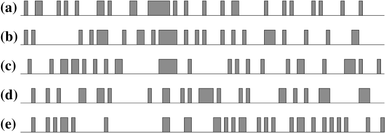
Figure 5: Random configurations obtained for $L=100$ and $\rho=0.3$. The largest cluster is of size a) 6, b) 5, c) 5, d) 4, e) 2. The shaded areas represent the location of the scatterers on the lattice.

configuration	Ruelle pressure	M	estimate
(a)	0.59532	6	0.589
(b)	0.56275	5	0.549
(c)	0.55034	5	0.549
(d)	0.50916	4	0.481
(e)	0.35389	2	0.000

Table 1: For the random configurations of figure 5, with $L=100$ and $\rho=0.3$, we compare the actual Ruelle pressure $\psi(\beta)$ with the estimate $\ln\Lambda(\beta;q_{M})$ based on the largest cluster size $M$, for $\beta=0$. PBC are used for configurations (a), (b), (c), and ABC for (d), (e). The corresponding mean–field values, $\psi_{MF}(0)=0.2079$ (PBC) and $\psi_{MF}(0)=0.2078$ (ABC), do not provide a sensible estimate.

6.1 Bounds on Ruelle pressure.

In [6, 1], it has been shown that the Ruelle pressure is bounded by

$$\ln\Lambda(q_{M})\simeq\ln(a+b)-\frac{a}{2b}\pi^{2}/M^{2}\;\leq\;\psi_{L}(\beta,\rho) \leq\ln(a+b)\qquad (\beta<1)$$

$$\beta(\ln q)\;1/\overline{M}\;\leq\;\psi_{L}(\beta,\rho) \leq\;\;0\qquad (\beta>1),$$

where $M$ is the size of the largest cluster and $\overline{M}$ of the largest void. The upper bound is a direct consequence from the inequalities

$$a+b>1\;\;\;\; \beta<1$$ if (58)

$$a+b<1\;\;\;\; \beta>1,$$ if (59)

and we refer to [6, 1] for more details. For $\beta<1$ (respectively $\beta>1$) the lower bound is the Ruelle pressure obtained by keeping only the largest cluster of the configuration (or respectively the largest void, bordered by 2 scatterers) and using ABC. In subsections 3.2, 3.3, and 6, we have found that for $\beta<1$, this is not only a lower bound but also a good estimate for the Ruelle pressure, as soon as $L$ is large enough. A consequence is that, among all possible configurations, the configuration with all scatterers solidly packed in a single cluster gives the maximum value of the Ruelle pressure. On the other hand, the minimum value is obtained for the mean field configuration with scatterers spaced at regular intervals of length $R=1/\rho$.

As a confirmation, we have verified (see fig. 6) that in a given set of $1000$ configurations, the largest eigenvalue for $\beta<1$ did correspond to a configuration where all scatterers are essentially packed together, whereas the lowest value was obtained for an “almost mean-field” configuration, i.e. the distance between scatterers is more or less constant. This is in agreement with our expectations [1]. To illustrate localization in these configurations, we have plotted the invariant vector $v_{+}(r)u_{+}(r)$ as a function of $r$ (figures 7 and 8). For configuration (a), the eigenvector is entirely localized on the large cluster on the left. Configuration (b), which is more of mean-field type, correspond more or less to an extended state. However, there is still partial localization in regions of higher than average density.

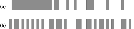
Figure 6: Among $1000$ random configurations generated for $L=50$, $N=25$, we select the configuration corresponding to the largest (a) and smallest (b) $\Lambda$–value, as determined numerically. The shaded areas correspond to the location of scatterers.

Figure 7: Invariant measure $\pi(x)$ of Eq. (25) for configuration (a) of figure 6. A thin line indicates the profile for the location of scatterers.

Figure 8: Invariant vector for configuration (b) of figure 6. A thin line indicates the profile for the location of scatterers.

7 Distribution of largest cluster size

Up till now we have studied single configurations. In the next sections we will present results averaged over the disorder and compare them with the upper and lower bounds in Eq. (LABEL:bounds). To do so, we need to average equation (LABEL:bounds) over all possible configurations of scatterers with a fixed density $\rho$ (or a fixed $N$) and a fixed system size $L$. In order to determine $\langle 1/M^{2}\rangle_{\rho}$ and $\langle 1/\overline{M}\rangle_{\rho}$, we have used three different estimates for the distribution of the largest cluster size. Note that the distribution for the size of the largest void is the same, upon exchanging scattering sites and empty sites. The first estimate, which is the most crude one, is just the distribution for having at least one cluster of size $M$ given by

$$P_{1}(M)=L\frac{\left(\begin{array}[]{c}L-M-2\\ N-M\end{array}\right)}{\left(\begin{array}[]{c}L\\ N\end{array}\right)}$$ (60)

This expression is valid only for large $M$ and for periodic boundary conditions. The numerator in (60) represents the number of ways one can distribute the $N-M$ remaining scatterers among the $L-M-2$ remaining empty sites, once a cluster of size $M$ limited by two empty border sites has been put in one of the $L$ possible locations. The denominator is the total number of possible configurations.

The calculation of the distribution of largest cluster sizes can be improved in the following way: Let $A(M)$ be the fraction of realizations with no cluster larger than $M$. Then

$$A(M-1)=A(M)\times[1-P_{1}(M)].$$ (61)

Note that $1-P_{1}(M)$ is the probability that there is no cluster of size $M$. This recursion relation can be solved by iteration starting at $M=N$, where $A(N)=1$. The result is :

$$A(M)=\Pi^{N}_{m=M+1}\left(1-P_{1}(m)\right).$$ (62)

The probability that the largest cluster size is $M$ is then

$$P_{2}(M)=A(M)-A(M-1)=P_{1}(M)\Pi^{N}_{m=M+1}\left(1-P_{1}(m)\right).$$ (63)

This expression for $P_{2}(M)$ can be calculated numerically for each system size, by using the factorial expression given above for $P_{1}(M)$. This is the second expression which was used for the numerical evaluation of lower bounds.

The third distribution $P_{3}(M)$ for the largest cluster considered here was obtained by simple generating a large number of configurations and finding the largest cluster for each of them.

Figure 9 compares these three estimates for the distribution when $\rho=0.4$, and $L=100$. As $P_{1}(M)$ is not bounded, it is cut off such that the probability is normalized. The distribution $P_{2}(M)$ has also to be cut off, otherwise it oscillates between unphysical positive and negative values at small $M$ (but we stress again that the formulas (60) and (63) are not valid for small $M$–values). The third distribution $P_{3}(M)$ has been averaged over $20000$ configurations.

Figure 9: Probability distribution for the largest cluster size $M$ in a system of size $L=100$, and $\rho=0.4$. The dotted, dashed, and solid lines correspond respectively to $P_{1}(M)$, $P_{2}(M)$, and the direct measurement $P_{3}(M)$ obtained by generating 20 000 random configurations.

We now verify that the largest cluster size grows as $\ln L$ for large $L$. Figure 10 shows $P_{2}(M)$ for increasing system sizes. The system size is varied from $100$ to $10^{8}$ and is multiplied by $10$ between each successive estimation. We check that each time the size $L$ is multiplied by $10$, the maximum of the distribution is shifted to the right by a constant value. Another verification is made by plotting the second moment $\langle 1/M^{2}\rangle_{2}$ calculated with the $P_{2}$–distribution as a function of $(\log_{10}L)^{-2}$ (see figure 11).

Figure 10: Probability distribution $P_{2}(M)$ for the largest cluster size $M$ for $\rho=0.4$, $\beta=0$, PBC, and for system sizes $L$ increasing geometrically from $100$ to $10^{8}$.

Figure 11: Scaling properties of the second moment $\langle 1/M^{2}\rangle_{2}$, calculated from figure 10, as a function of $1/(\log_{10}L)^{2}$ for $L=100$ to $10^{8}$, at $\rho=0.4$ and $\beta=0$.

As already discussed in [1], it is possible in the one–dimensional case for $\beta<1$ and $L$ not too large, that the Ruelle pressure is not determined by the largest cluster but by a “dominant” cluster with average density $\rho+\Delta\rho$ intermediate between $\rho$ and $1$. This is indeed what is observed in numerical simulations. At $\beta=0$ and for $L=100$, we have taken all segments of all lengths, measured the average density on each of them, calculated the corresponding Ruelle pressure using the mean field expression (33), and kept the one which gives the largest value. We call it the dominant cluster. For some configurations it coincides with the largest cluster, but not always. Figure 12 compares the distributions for dominant and largest clusters. They are different, the first one being slightly shifted towards larger values. Note that a cluster, dominant for a given $\beta$, may not be dominant for another $\beta$ value.

Another illustration of partial localization in high density regions instead of solid clusters was given by figure 8.

Figure 12: Probability distribution for the largest (solid line) and dominant (dashed line) cluster size in a system of size $L=100$, for $\rho=0.4$ and $\beta=0$. These distributions were obtained by generating 20 000 random configurations.

8 Average Ruelle pressure.

Now we can use any of the three estimates for the distribution to calculate the average (LABEL:bounds) over all possible configurations and compare the resulting lower and upper bounds with the numerical measurements of the Ruelle pressure. For fixed $L$ and $\rho$, a large number of scatterer configurations has been generated, and for each of them the largest eigenvalue has been calculated. The average of its logarithm yields a numerical value for the Ruelle pressure.

We first consider the case where $\beta<1$. We have collected data for $\beta=0$, for which the Ruelle pressure equals the topological entropy. Figure 13 confirms that numerical data are between the upper and lower bounds. The lower bounds based on any of these three distributions are qualitatively the same.

Figure 13: Ruelle pressure $\psi(\beta=0)$ (solid line) for $L=100$, as a function of the density $\rho$, compared with upper (dotted line) and lower bounds (dashed lines). For comparison, the mean field prediction has also been indicated (dashed–dotted line).

The estimate for the largest cluster distribution, especially the one based on $P_{1}(M)$, may seem rather crude. In fact, most of the system sizes that we are able to explore numerically are too small for the Ruelle pressure to be entirely dominated by the largest cluster, and no improvement of the estimates for $P(M)$ is likely to make the quantitative agreement better.

However, when the system size is increased ($L=10000$), we check –within the precision of our measurements– that the lower bound based on the largest cluster approximation is indeed a good estimate of the Ruelle pressure (figure 14). It should be noted that at $\beta=0$, the Ruelle pressure is independent of $p$ and $q$, and thus these results are valid both for large or small $q$.

Figure 14: Ruelle pressure $\psi(\beta=0)$ (solid line) for $L=10000$, as a function of the density $\rho$, compared with upper (dotted line) and lower bounds (dashed lines). For comparison, the mean field prediction has also been indicated (dashed–dotted line).

One can also verify that for a given system size, the mean field prediction gives a value much lower than the average, whereas the configuration with all scatterers are solidly packed together has a Ruelle pressure almost equal to the upper bound. This is illustrated in figure 15 for $L=400$. Thus for a configuration with $L=400$ and a given density, any value between the two dashed–dotted lines of figure 15 can be realized.

Figure 15: Ruelle pressure $\psi(\beta=0)$ as a function of the density $\rho$ for $L=400$. The solid line is an average over $10000$ configurations. The dashed–dotted lines are the extreme values obtained for specific configurations, namely the ‘mean field’ configuration and the one where all scatterers are packed together in a solid cluster. The upper bound $\psi(0)=\ln 2$ is also indicated.

Now we address the case $\beta>1$. Tables 2 and 3 give some numerical values for the measured or estimated Ruelle pressure, and for the mean field prediction (33), in the case of $L=100$ and $\beta=2$. When $q$ is large (table 2), the lower bound is not only a lower bound but also a good estimate of the Ruelle pressure, and is much lower than the mean-field value. The numerical data are also displayed in figure 16.

Figure 16: Ruelle pressure as a function of the system size in the case of strong backscattering ($p=0.2$) for $\rho=0.2$ ($\circ$) or $\rho=0.8$ ($\Box$). Lower bounds (solid lines) were obtained using a numerical determination of the largest cluster size distribution.

When $q$ is small (table 3, figure 17), the situation is reversed. A good estimate is obtained by using the mean field theory result, while the theoretical lower bound differs significantly from the measured Ruelle pressure. We may roughly estimate under which condition the lower bound will be a better estimate than the mean field theory by comparing the corresponding eigenvalues in (LABEL:bounds) and (32) with $R=1/\rho$ :

$$q^{\beta/\overline{M}}<(a+b)^{\rho}$$ (64)

or with $b=q^{\beta}$

$$\overline{M}>\frac{|\ln b\,|}{\rho|\ln(a+b)\,|}.$$ (65)

If $p>q$, then for $\beta>>1$ we have $a>>b$. Localization will dominate over mean field if

$$\overline{M}>\frac{|\ln b|}{\rho|\ln a|}=\frac{|\ln q|}{\rho|\ln p|},$$ (66)

i.e. the system size $L$ must be typically larger than $\exp(1/\rho\;\ln q/\ln p)$. On the other hand, at fixed $L$, $\beta$ must be larger than

$$\beta>1+\frac{(\ln q)|\ln(1-\rho)|}{(p\ln p+q\ln q)\rho M}$$ (67)

where $M\sim\ln L$. This results from an expansion in powers of $\beta-1$ [1]. It appears that, if $q$ is small, it is necessary to go to very large $L$ and/or $\beta$ values to see the occurrence of localization. In the case of figure 17, $\beta=2.0$ and $L=400$ are not large enough to see this phenomenon. Figure 18 shows that this is also the case for a different density $\rho$.

Figure 17: Ruelle pressure as a function of the system size in the case of weak backscattering ($p=0.8$) at a high density $\rho=0.8$ ($\triangle$). The lower bound (dashed line) was obtained using a numerical determination of the largest cluster size distribution. The mean field prediction (dashed–dotted line) is a much better estimate for the Ruelle pressure.

Figure 18: Ruelle pressure as a function of the system size in the case of weak backscattering probability ($p=0.8$) at a low density $\rho=0.2$ ($\triangle$). Again, the mean field prediction (dashed–dotted line) is a much better estimate for the Ruelle pressure.

$\rho$	0.2	0.5	0.8
Numerical value	0.02809	0.06583	0.12211
Lower bound	0.02851	0.06682	0.12406
Mean field	0.07713	0.19283	0.30853

Table 2: For $p=0.2$ (large backscattering probability), the Ruelle pressure, evaluated numerically by averaging over 10 000 configurations, is compared to the lower bound and the mean field value, for different densities of scatterers and a system size $L=100$.

$\rho$	0.2	0.5	0.8
Numerical value	0.07218	0.17361	0.29033
Lower bound	0.20584	0.48190	0.91901
Mean field	0.07713	0.19283	0.30853

Table 3: For $p=0.8$ (weak backscattering probability), the Ruelle pressure, evaluated numerically by averaging over 10 000 configurations, is compared to the lower bound and the mean field value, for different densities of scatterers and a system size $L=100$.

The picture of what happens when $p>q$ can still be refined. The crossover between trajectories extended over the whole lattice (mean field) and trajectories localized in the largest void (lower bound) is in fact not direct. Some intermediate semi–localization may occur. As mentioned in section 7, this was already evidenced for one–dimensional systems at $\beta<1$ (and for all $p,q$ values) [1]. We will show now that a similar phenomenon occurs for $\beta>1$ when $p>q$. We then have not only $a>>b$, but also $a<<1$ ($\beta>1$). Thus (i) on the one hand the particle has a tendency to escape from the void because back-scattering is weak; (ii) on the other hand, as $a<<1$, the free propagation is till favored over forward propagation through a scatterer. If $a\simeq 1$, the second effect is negligeable and the mean field prediction will be appropriate, as it is the case in figures 17 and 18. If $a<<1$, the competition between the two effects may eventually promote some intermediate configurations. As an illustration, we will consider the configuration of figure 19 : the whole lattice is solidly filled with scatterers except in the low density region of size $R$. In this region, $n$ isolated scatterers are placed at equal distance from each other. We will compare the weights of a trajectory $T_{1}$ undergoing only free propagation and back–scattering, i.e. confined in a void in a strict sense between two isolated scatterers; and a trajectory $T_{2}$ going through the $n$ isolated scatterers and thus exploring the entire low density region of size $R$.

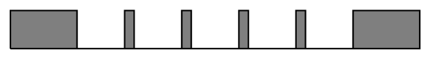
Figure 19: Special configuration, in which a trajectory exploring the whole low density region may have a higher weight if $p>q$ than a trajectory remaining in one of the voids.

During $t$ time steps, $T_{1}$ will undergo $t/[R/(n+1)]$ back–scatterings, while $T_{2}$ will undergo $t/R$ back–scatterings and $tn/R$ forward–scatterings. Thus $T_{2}$ has a higher weight than $T_{1}$ if

$$q^{\beta\frac{t}{R}}p^{\beta\frac{tn}{R}}>q^{\beta\frac{t(n+1)}{R}}$$ (68)

or equivalently $p>q$. This shows that as soon as $p>q$, localization may occur not in the largest void but in a large low density region. However, when $L$ increases, we speculate that it is more and more likely to find a large void that will nevertheless dominate the result.

9 Conclusion

We conclude this paper with a number of remarks:

1) We have shown that the Ruelle pressure of Lorentz lattice gases in the limit of infinite systems is completely determined by rare fluctuations in the configuration of scatterers. Thus it carries no information on the global structure of the disorder. Numerical studies allowed us to show that this also holds for finite but large systems, for all but a small range of $\beta$ values. Then we were able to predict quantitatively the Ruelle pressure for all $\beta$ except for a small region around $\beta=1$.

As already discussed in [6], these results can be immediately generalized to a whole class of diffusive systems with static disorder. The special case of a continuous Lorentz gas has been briefly considered in [1].

Localization phenomena in fact appear very often in physics, as soon as there is some competition between energetically favorable configurations and entropic effects. Some localization effects were already shown in the framework of the thermodynamic formalism for deterministic maps [2] or multifractals [4]. However, it is the first time that such effects are evidenced in hard spheres systems as resulting from the quenched disorder. Localization occurs on the most extreme fluctuation of the disorder. For infinitely large systems, this fluctuation may be arbitrarily large, which allows for a very pronounced effect.

2) The Ruelle pressure is a characteristic of the dynamics of the system not only for the isolated $\beta$ values where a direct interpretation can be given (see section 2), but also as a whole. In the same way, in a power spectrum, only some of the points may receive an individual interpretation, but the whole structure of the spectrum is interesting. An open question is to know if enough information has been kept in the region around $\beta=1$ where delocalization does not occur, in order to be able for example to reconstruct the structure of the disorder from it. To this respect, it would be interesting to rescale the region around $\beta=1$ as the system size increases, in order to prevent it from shrinking to zero in the thermodynamic limit. The scaling of this region with the system size has been estimated in [1].

When localization occurs, the information contained in the Ruelle pressure concerns the properties of individual scatterers. More precisely, the knowledge of the $\beta$ regions in which one given type of scatterers will dominate yields a measure of what could be called the isotropy of the different scatterers.

3) Numerical studies have been performed only in one dimension. Analytical results showed that the localization occurring in the thermodynamic limit and the extension of the delocalized region around $\beta=1$ can be generalized to higher dimensions. Localization occurs also for finite but large systems. The only difference with the one–dimensional case is that now the lower bound may not be a good estimate for the Ruelle pressure at finite size. Indeed, the lower bound chosen here was based on localization in hypercubic domains. In fact, it may happen on domains with much more general shapes.

Acknowledgments: The numerical values for the Ruelle pressure in figure 13 and table 1 were obtained by C. Bokel. We thank J.R. Dorfman and H. van Beijeren for a fruitful collaboration, and H.A. van der Vorst and G.L.G. Sleijpen for useful discussions about iterative methods. C. Appert acknowledges support of the foundation “Fundamenteel Onderzoek der Materie” (FOM), which is financially supported by the Dutch National Science Foundation (NWO), and of the “Centre National de la Recherche Scientifique” (CNRS).

Appendix A

In the case of $N$ scatterers packed in a single cluster in a system of size $L=N+R-1$ with PBC, a perturbative calculation for the largest eigenvalue $\Lambda$ has been presented in section 3.2. Here we calculate the largest eigenvalue directly from the set of equations (34).

First notice that the bulk equations in (34) impose the relation (43) between $\Lambda$ and the wave number $q$, as can be found in a similar way as equation (27). Now the wavenumber $q$ has to be determined from the boundary equations

$$\Lambda^{R}U_{+}(1) = aU_{+}(N)+bU_{-}(N)$$

$$\Lambda U_{-}(1) = bU_{+}(2)+aU_{-}(2)$$

$$\Lambda U_{+}(N) = aU_{+}(N-1)+bU_{-}(N-1)$$

$$\Lambda^{R}U_{-}(N) = bU_{+}(1)+aU_{-}(1)$$ (69)

We search for a solution of the form

$$U_{+}(k)=A\exp[\imath q(k-1)]+c.c.$$

$$U_{-}(k)=B\exp[\imath q(N-k)]+c.c.$$ (70)

By inserting this form into (69), we obtain four equations which determine A and B (complex numbers). Non trivial solutions exist only if the determinant of the system vanishes. This yields a transcendental equation for $q$ which can be solved using the ansatz

$$q=\frac{\pi}{N-1+\delta}.$$ (71)

This ansatz is based on the assumption that the present case is similar to ABC, as soon as $R$ is large enough. This will be correct only for $\beta<1$.

The determinant is expanded in powers of $q$. Replacing $\Lambda$ by its expression (43) in terms of $q$, we find:

Det $$= -4\,q^{2}\,(\delta b-a+b)(\Lambda^{R}+a+b)$$ (72)

$$\times\left[\delta\,b\,(\Lambda^{R}-a-b)\,-\,(a+b)(\Lambda^{R}+a-b)\right].$$

Setting this determinant equal to zero yields two solutions. We select the one that gives the smallest $q$, i.e. the largest eigenvalue, and find expression (44).

Appendix B : Recurrence formula for the determinant of $w$

For a one–dimensional system, the transition matrix has a form such that an exact recursion relation can be found to calculate its determinant. We will first illustrate it for ABC. The transition matrix is of the form

$$w=\left(\begin{array}[]{ccccccccccc}\Lambda&b_{2}&a_{2}&&&&&&&&\\ b_{1}&\Lambda&&&&&&&&&\\ &&\Lambda&b_{3}&a_{3}&&&&&&\\ &a_{2}&b_{2}&\Lambda&&&&&&&\\ &&&&\Lambda&b_{4}&&&&&\\ &&&a_{3}&b_{3}&\Lambda&&&&&\\ &&&&&&\cdots&&&&\\ &&&&&&&\Lambda&b_{L-1}&a_{L-1}&\\ &&&&&&&b_{L-2}&\Lambda&&\\ &&&&&&&&&\Lambda&b_{L}\\ &&&&&&&&a_{L-1}&b_{L-1}&\Lambda\end{array}\right)$$ (73)

If the $k$-th scatterer is located in site $j$, we define $D_{k}$ as the determinant of the $2j-1$ first lines and columns. An auxiliary quantity $E_{k}$ is obtained from $D_{k}$ by removing the last column and the last but one line. Then the following recursion relations hold :

$$D_{k+1} = \Lambda^{2R_{k}}D_{k}-bE_{k+1}$$

$$E_{k+1} = bD_{k}+a^{2}E_{k}.$$ (74)

Using the initial conditions

$$D_{1} = \Lambda^{1+2R_{o}}$$

$$E_{1} = 0,$$ (75)

we can iterate the equations (74) and find the determinant for the whole matrix $w$ as

$$\mbox{Det}(w)=\Lambda^{1+2R_{N}}D_{N}.$$ (76)

The recursive calculation is performed numerically. For $\beta=0$ (i.e. $\Lambda\simeq 2$), it is possible to calculate the determinant for matrices up to size $4(L-1)^{2}$, beyond which the method is spoiled by numerical overflow problems.

In the case of PBC, the recursion relations are slightly more complicated. The matrix $w$ is now of size $4L^{2}$ and reads

$$w=\left(\begin{array}[]{ccccccccccccc}\Lambda&&&&&&&&&&&a_{L}&b_{L}\\ &\Lambda&b_{2}&a_{2}&&&&&&&&&\\ a_{1}&b_{1}&\Lambda&&&&&&&&&&\\ &&&\Lambda&b_{3}&a_{3}&&&&&&&\\ &&a_{2}&b_{2}&\Lambda&&&&&&&&\\ &&&&&\Lambda&b_{4}&&&&&&\\ &&&&a_{3}&b_{3}&\Lambda&&&&&&\\ &&&&&&&\cdots&&&&&\\ &&&&&&&&\Lambda&b_{L-1}&a_{L-1}&&\\ &&&&&&&&b_{L-2}&\Lambda&&&\\ &&&&&&&&&&\Lambda&b_{L}&a_{L}\\ &&&&&&&&&a_{L-1}&b_{L-1}&\Lambda&\\ b_{1}&a_{1}&&&&&&&&&&&\Lambda\end{array}\right)$$ (77)

We choose the origin of the lattice such that there is no scatterer in sites $1$ and $L$. For PBC, this is always possible if there are 2 holes in a row somewhere in the configuration, which will be the case for all configurations if $\rho<0.5$. Then $b_{1}=b_{L}=0$.

It can be shown that the determinant of $w$ is given by

$$\mbox{Det}(w)=\Lambda^{2R_{N}+1}D_{N}-bD^{*}_{N}-a^{2}E^{*}_{N}+2\Lambda(-\Lambda)^{L-1}a^{N},$$ (78)

where $D_{N}$ and $E_{N}$, $D^{*}_{N}$ and $E^{*}_{N}$, are obtained from the recurrence formula (74) with respectively the initial conditions (75) and

$$D^{*}_{1} = \Lambda^{2(R_{o}-1)}b_{2}-bE^{*}_{1}$$

$$E^{*}_{1} = {b_{2}}^{2}-{a_{2}}^{2}.$$ (79)

Appendix C : Arnoldi’s method

Consider an $n\times n$ matrix $A$.

We start from a guess $u_{o}$ for the right eigenvector. In a classical power method, one would apply the matrix $A$ repeatedly to this vector until it is aligned with the eigenvector associated with the largest eigenvalue. With Arnoldi’s method, we built a basis of $m$ vectors that will span the vector–space more rapidly. If $j$ vectors $\{u_{o},u_{1},\cdots,u_{j-1}\}$ of the basis have been obtained already, $u_{j}$ is defined as follows. First matrix $A$ is applied :

$$u^{\prime}_{j}=Au_{j-1}.$$ (80)

Then $u^{\prime}_{j}$ is orthogonalized with respect to the $j$ first vectors :

$$u^{\prime\prime}_{j}=u^{\prime}_{j}-\sum_{k=0}^{j-1}\left[u^{\prime}_{j}.u_{k}\right]u_{k}.$$ (81)

Finally, $u_{j}$ is equal to the normalized $u^{\prime\prime}_{j}$. This process is iterated until $m$ vectors are obtained.

A reduced $m\times m$ matrix $H$ is defined by

$$h_{ij}=u^{i-1}u^{j},$$ (82)

such that

$$A={\cal U}H{\cal U}^{T}+B,$$ (83)

where ${\cal U}=\{u_{o},u_{1},\cdots,u_{m}\}$, and $B$ is expected to be small. Notice that the definition of $H$ implies that $h_{j+1,j}$ is the norm of $u^{\prime\prime}_{j}$, and $h_{ij}=0$ if $i>j+1$. As a consequence it is straightforward to calculate the determinant of $H$, and thus to find its largest eigenvalue $\Lambda$ by Newton’s method (we know that it is smaller than $a+b$) and the associated eigenvector $y_{H}$. The first approximation for the largest eigenvalue of $w$ is taken to be $\Lambda$ associated with ${\cal U}h_{H}$. If it is not satisfactory, the whole process is repeated, taking ${\cal U}h_{H}$as a new initial guess. The size $m$ of the basis has to be tuned in order to optimize the efficiency of the method.

A difficulty that this method shares with other iterative methods occurs when the largest eigenvalue is almost degenerate with the next smaller one. Then we may by mistake converge towards the second one. However, this is not a real problem as long as we are interested in the eigenvalue itself.

It should also be noted that, as usual, convergence theorems exist only for symmetric matrices, whereas the method has been applied here to non–symmetric matrices.

References

- [1] C. Appert, H. van Beijeren, M.H. Ernst, and J.R. Dorfman. Thermodynamic formalism and localization in Lorentz lattice gases. to appear in J. Stat. Phys, vol. 87, 1996.
- [2] C. Beck and F. Schlögl. Thermodynamics of chaotic systems. Cambridge U. Press, 1993.
- [3] David Ruelle. Thermodynamic Formalism. Addison Wesley Publ. Co. (Reading, Mass, 1978)., 1978.
- [4] M.J. Feigenbaum, I. Procaccia, and T. Tél. Scaling properties of multifractals as an eigenvalue problem. Phys. Rev. A, 39:5359, 1989.
- [5] P. Gaspard and F. Baras. Chaotic scattering and diffusion in the Lorentz lattice gas. Phys. Rev. E, 51:5332, 1995.
- [6] C. Appert, H. van Beijeren, M.H. Ernst, and J.R. Dorfman. Thermodynamic formalism in the thermodynamic limit: Diffusive systems with static disorder. PRE, 54:R1013, 1996.
- [7] P. Gaspard and G. Nicolis. Phys. Rev. Lett., 65:1693, 1990.
- [8] M.H. Ernst and J.R. Dorfman. Chaos in Lorentz lattice gases. In J.J. Brey, J. Marro, J. M. Rubi, M. San Miguel editors, editor, 25 Years of Non-Equilibrium Statistical Mechanics, pages 199–210. Springer Verlag, Berlin, 1995.
- [9] P. Gaspard and B. Dorfman. Chaotic scattering theory, thermodynamic formalism, and transport coefficients. Phys. Rev. E, 52:3525, 1995.
- [10] M.H. Ernst, J.R.Dorfman, R. Nix, and D. Jacobs. Mean field theory for Lyapunov exponents and Kolmogorov-Sinai entropy in Lorentz lattice gases. Phys. Rev. Lett., 74:4416, 1995.
- [11] H. van Beijeren and H. Spohn. Transport properties of the one-dimensional stochastic lorentz model - i, velocity autocorrelation function. J. Stat. Phys., 31:231–254, 1983.
- [12] J.R. Dorfman, M.H. Ernst, and D. Jacobs. Dynamical chaos in the Lorentz lattice gas. J. Stat. Phys., 81:497–513, 1995.
- [13] Y. Saad. Numerical methods for large eigenvalue problems. revised version (unpublished), 1995.