On the number of limit cycles of the Liénard equation
H. Giacomini and S. Neukirch
Laboratoire de Mathématiques et Physique Théorique
C.N.R.S. UPRES A6083
Faculté des Sciences et Techniques, Université de Tours
F-37200 Tours FRANCE

Abstract

In this paper, we study a Liénard system of the form $\dot{x}=y-F(x)\;,\;\dot{y}=-x$, where $F(x)$ is an odd polynomial. We introduce a method that gives a sequence of algebraic approximations to the equation of each limit cycle of the system. This sequence seems to converge to the exact equation of each limit cycle.
We obtain also a sequence of polynomials $R_{n}(x)$ whose roots of odd multiplicity are related to the number and location of the limit cycles of the system.

PACS numbers : 05.45.+b , 02.30.Hq , 02.60.Lj , 03.20.+i

Key words : Liénard equation, limit cycles. A two-dimensional autonomous dynamical system is defined by two coupled first order differential equations of the form :

$$\dot{x}=P(x,y)\quad,\quad\dot{y}=Q(x,y)$$ (1)

where $P$ and $Q$ are two functions of the variables $x$ and $y$ and the overdots denote a time derivative.

Such a type of dynamical system appears very often within several branches of science, such as biology, chemistry, astrophysics, mechanics, electronics, fluid mechanics, etc [1, 2, 3, 4, 5, 6].

One of the most difficult problems connected with the study of system (1) is the question of the number of limit cycles. A limit cycle is an isolated closed trajectory. Isolated means that the neighboring trajectories are not closed; they spiral either toward or away from the limit cycle. If all neighboring trajectories aproach the limit cycle, we say that the limit cycle is stable or attracting. Otherwise the limit cycle is unstable or, in exeptional cases, half-stable. Stable limit cycles are very important in science. They model systems that exhibit self-sustained oscillations. In other words, these systems oscillate even in the absence of external periodic forcing. Of the countless examples that could be given, we mention only a few : the beating of a heart, chemical reactions that oscillate spontaneously, self-excited vibrations in bridges and airplane wings, etc. In each case, there is a standard oscillation of some preferred period, waveform and amplitude. If the system is slightly perturbated, it always returns to the standard cycle. Limit cycles are an inherently nonlinear phenomena; they cannot occur in linear systems [7, 8, 9, 10, 11, 12].

The first physical model to appear in the literature which can be transformed to a system of type (1) containing a limit cycle is due to Rayleigh [13]. The following equation :

$$\frac{d^{2}y}{dt^{2}}+\epsilon\left(\frac{1}{3}(\frac{dy}{dt})^{3}-\frac{dy}{dt}\right)+y=0$$ (2)

that originated in connection with a theory of the oscillation of a violin string, was derived by Rayleigh in 1877.

In 1927, the dutch scientist van der Pol [14] described self-excited oscillations in an electrical circuit with a triode tube with resistive properties that change with the current. The equation derived by van der Pol reads :

$$\frac{d^{2}x}{dt^{2}}+\epsilon(x^{2}-1)\frac{dx}{dt}+x=0$$ (3)

Equations (2) and (3) are equivalent, as can be seen by differentiating (2) with respect to $t$ and putting $\frac{dy}{dt}=x$.

In 1928, the french engineer A. Liénard [15] gave a criterion for the uniqueness of periodic solutions for a general class of equations, for which the van der Pol equation is a special case :

$$\frac{d^{2}x}{dt^{2}}+f(x)\frac{dx}{dt}+x=0$$ (4)

Liénard tranformed (4) to a first order system by setting $\frac{dx}{dt}=z$, yielding

$$\frac{dx}{dt}=z\quad,\quad\frac{dz}{dt}=-x-f(x)z$$ (5)

In fact, in his proof, Liénard used a form equivalent to (5), obtaining through the change of variable $z=y-F(x)$, where $F(x)=\int_{0}^{x}f(\tau)d\tau$ :

$$\frac{dx}{dt}=y-F(x)\quad,\quad\frac{dy}{dt}=-x$$ (6)

Equation (4) is referred to as Liénard equation and both system (5) and (6) are called Liénard systems. They are a particular case of (1).

In 1942, Levinson and Smith [16] suggested the following generalization of system (6) :

$$\frac{dx}{dt}=y-F(x)\quad,\quad\frac{dy}{dt}=-g(x)$$ (7)

or equivalently :

$$\frac{dx}{dt}=z\quad,\quad\frac{dz}{dt}=-g(x)-f(x)z$$ (8)

Sytems (7) and (8) are equivalent to :

$$\frac{d^{2}x}{dt^{2}}+f(x)\frac{dx}{dt}+g(x)=0$$ (9)

which is sometimes referred to as the generalized Liénard equation.

In this paper, we will consider the case $g(x)=x$ and $F(x)$ given by an arbitrary odd polynomial of degree $m$. The fundamental problem for this type of system is the determination of the number of limit cycles for a given polynomial $F(x)$ [17, 18, 19, 20, 21, 22, 23, 24] . For $m=3$, i.e. for $F(x)=a_{1}x+a_{3}x^{3}$, it has been shown in [17] that the system has a unique limit cycle if $a_{1}a_{3}<0$ and no limit cycle if $a_{1}a_{3}>0$. For $m=5$ it has been shown in [25] that the maximum number of limit cycles is two. For $m>5$, there are no general results about the number of limit cycles of (6).

In this paper, we present a new method that gives information about the number of limit cycles of (6) and their location in phase space, for a given odd polynomial F(x). This method gives also a sequence of algebraic approximations to the cartesian equation of the limit cycles.

We will explain our method through the analysis of a very well known case, the van der Pol equation. In this case, we have :

$$F(x)=\epsilon(x^{3}/3-x)$$ (10)

We propose a function $h_{2}(x,y)=y^{2}+g_{1,2}(x)y+g_{0,2}(x)$, where $g_{1,2}(x)$ and $g_{0,2}(x)$ are arbitrary functions of $x$. Here, the second subindex makes reference to the degree of the polynomial $h_{2}$ with respect to the $y$ variable. Then we calculate $\dot{h_{2}}=(y-F(x))\frac{\partial h_{2}}{\partial x}-x\frac{\partial h_{2}}{\partial y}$. This quantity is a second degree polynomial in the variable $y$. We will choose $g_{1,2}(x)$ and $g_{0,2}(x)$ in such a way that the coefficients of $y^{2}$ and $y$ in $\dot{h_{2}}$ are zero. From these conditions , we obtain $g_{1,2}(x)=k_{1}$ and $g_{0,2}(x)=x^{2}+k_{0}$, where $k_{0}$ and $k_{1}$ are arbitrary constants. As $F(x)$ is an odd polynomial, if $(x,y)$ is a point of the limit cycle of (6), then the point $(-x,-y)$ also belongs to this limit cycle. The equation of a limit cycle of (6) must be invariant by the transformation $(x,y)\rightarrow(-x,-y)$. We want the function $h_{2}(x,y)$ to have this symmetry too. Thus we take $k_{1}=0$. We then have $\dot{h_{2}}=R_{2}(x)=-2xF(x)=-2\epsilon x^{2}(x^{2}/3-1)$. The polynomial $R_{2}(x)$ is even and it has exactly one positive root of odd multiplicity, i.e. $x=\sqrt{3}$.

If we integrate the function $\dot{h_{2}}$ along the limit cycle, we have : $\int_{0}^{T}\dot{h_{2}}(x(t),y(t))dt=\int_{0}^{T}R_{2}(x(t))dt$ , where T is the period; but $\int_{0}^{T}\dot{h_{2}}(x(t),y(t))dt=h_{2}(x(T),y(T))-h_{2}(x(0),y(0))=0$. Consequently, we find : $\int_{0}^{T}R_{2}(x(t))dt=0$. This last equality tells us that there cannot be any limit cycle in a region of the phase plane where $R_{2}(x)$ is of constant sign. For the van der Pol system, $R_{2}(x)$ has a root of odd multiplicity at $x=\sqrt{3}$ , hence the maximum value of $x$ for the limit cycle must be greater than $\sqrt{3}$. The curves defined by $h_{2}(x,y)=x^{2}+y^{2}+k_{0}=0$ are closed for $k_{0}<0$.

As the next step of our procedure, we propose a fourth degree polynomial in $y$ for the function $h_{4}(x,y)$, i.e. $h_{4}(x,y)=y^{4}+g_{3,4}(x)y^{3}+g_{2,4}(x)y^{2}+g_{1,4}(x)y+g_{0,4}(x)$ (polynomials $h_{n}(x,y)$ with $n$ odd do not give useful information about the limit cycles of the system since the level curves $h_{n}(x,y)$ are open and the polynomials $R_{n}(x)$ have always a single root of odd multiplicity at $x=0$) . By imposing the condition that $\dot{h_{4}}$ must be a function of only $x$, we find $\dot{h_{4}}=R_{4}(x)$, where $R_{4}(x)$ is an even polynomial of tenth degree. The roots of $R_{4}(x)$ depend of $\epsilon$, hence in the following, we will take $\epsilon=1$. For this case, $R_{4}(x)$ has only one positive root of odd multiplicity, given by $x\simeq 1.824$. This root is greater than the root of $R_{2}(x)$. Obviously, the maximum value of $x$ for the limit cycle must be greater than this value.

We have in this way a new lower bound for the maximum value of $x$ on the limit cycle. Moreover the number of positive roots of odd multiplicity is equal to the number of limit cycles of the system. The condition that $\dot{h_{4}}$ must be a function only of $x$ imposes a first order trivial differential equation for each function $g_{j,n}(x)$. These equations can be solved by direct integration and we obtain in this way all the functions $g_{j,n}(x)$. We take all the integration constants, that appear when we solve these equations, equal to zero. In this way, the level curves $h_{4}(x,y)=K$ are all closed for positive values of $K$ and even values of $n$. Moreover, the function $h_{4}(x,y)$ is a polynomial in $x$ and $y$.

We have found the same results for greater values of $n$ even. We have calcultated $h_{n}(x,y)$ and $R_{n}(x)$ up to order 20. In all cases, the polynomials $R_{n}(x)$ have only one positive root of odd multiplicity. Let $r_{n}$ be the number of such roots. For the van der Pol equation, it seems that $r_{n}=1\;\forall n$ even. These roots approach in a monotonous fashion the maximum value of $x$ on the limit cycle. The functions $h_{n}(x,y)$ are polynomials in $x$ and $y$ for all $n$. The level curves $h_{n}(x,y)=K$ are all closed for positive values of K. By imposing the condition that the maximum value of $x$ on the curve $h_{n}(x,y)=K>0$ must be equal to the root of $R_{n}(x)$, we find a particular value of K for each $n$ even. Let us call this value $K_{n}^{\star}$. The level curve $h_{n}(x,y)=K_{n}^{\star}$ represents an algebraic approximation to the limit cycle.

In fig. 1 and 2 we show this curve for the values $n=6$ and $n=18$, respectively. In table 1 we give the values of the roots of $R_{n}(x)$ and the values of $K_{n}^{\star}$ for $2\leq n\leq 20$. The numerical value of the maximum of $x$ on the limit cycle, determined from a numerical integration of (6), with $F(x)$ defined by (10), is $x_{max}\simeq 2.01\;(\epsilon=1)$. It is clear that the roots of $R_{n}(x)$ seem to converge to $x_{max}$ and the curves $f_{n}(x,y)=K_{n}^{\star}$ seem to converge to the limit cycle.

We have also studied the case :

$$F(x)=0.8x-\frac{4}{3}x^{3}+0.32x^{5}$$ (11)

This system has exactly two limit cycles [18]. We have calculated the polynomials $h_{n}(x,y)$ and $R_{n}(x)$ up to $n=16$. The polynomials $R_{n}(x)$ have exactly two positive roots of odd multiplicity. We conjecture that $r_{n}=2\;\forall\,n$ even. For each value of $n$, we determine two values $K_{n1}^{\star}$ and $K_{n2}^{\star}$. The closed curves $h_{n}(x,y)=K_{n1}^{\star}$ and $h_{n}(x,y)=K_{n2}^{\star}$ provide algebraic approximations to each cycle for each value of $n$ even.

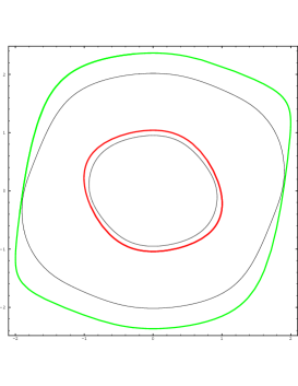
Figure 3: The limit cycles of equation (6) with $F(x)$ given by (11) (rough curves) and their algebraic approximations (smooth curves) : $h_{6}(x,y)=K_{6\,1}^{\star}$ and $h_{6}(x,y)=K_{6\,2}^{\star}$

In fig. 3 and 4 we show these curves for $n=6$ and $n=14$, respectively. We also show the limit cycles obtained by numerical integration. In table 2, we give the values of the roots of $R_{n}(x)$ and the values of $K_{n1}^{\star}$ and $K_{n2}^{\star}$ for $2\leq n\leq 16$. These roots seem to converge to the maximum values of $x$ for each cycle (the numerical values of the maximum of $x$ on each limit cycle are $x_{max,1}\simeq 1.0034$ and $x_{max,2}\simeq 1.9992$ respectively). The curves $h_{n}(x,y)=K_{n1}^{\star}$ and $h_{n}(x,y)=K_{n2}^{\star}$ seem to converge to each one of the limit cycles of the system.

For all the cases that we have studied, we have found that the values of the constants $K_{n}^{\star}$ go to zero or infinity when $n\rightarrow\infty$. In fact, it is easy to see from table 1 and table 2 that the asymptotic behaviour of $K_{n}^{\star}$ with $n$ (for a given limit cycle), is given by

$$K_{n}^{\star}\simeq a(x_{max})^{n}$$ (12)

where a is a constant which depends on the cycle (see fig. 5).

We have also considered system (6) with :

$$F(x)=x^{5}-\mu x^{3}+x$$ (13)

where $\mu$ is an arbitrary parameter. It has been proved in [25] that this system has exactly two limit cycles for $\mu>2.5$. It is clear that this system has no limit cycle for $\mu<2$ because $r_{2}=0$ in that case. Hence, between $\mu=2$ and $\mu=2.5$ there is a bifurcation value $\mu^{\star}$ such that for $\mu<\mu^{\star}$ the system has no limit cycles and for $\mu>\mu^{\star}$ the system has exactly two limit cycles. When $\mu=\mu^{\star}$ the system undergoes a saddle-node bifurcation.

By applying our method, we can obtain lower bounds for the value of $\mu^{\star}$. For each even value of $n$ we calculate the maximum value of $\mu$ for which $r_{n}$ is zero. This value of $\mu$ represents a lower bound for $\mu^{\star}$. The results of these calculations are given in table 3. The values of ${\mu}_{n}^{\star}$ seem to converge very quickly, in a monotonous way, when $n\rightarrow\infty$. Numerical integrations of system (6) with $F(x)$ given by (13) seem to confirm that $\lim_{n\rightarrow\infty}\mu_{n}^{\star}=\mu^{\star}$.

Let us point out that it is the first time, in our knowledge, that a bifurcation value of this type can be estimated in such a way, that is by employing an analytical method instead of a numerical integration of the system.

We have also analysed system (6) with $F(x)$ given by :

$$F(x)=x(x^{2}-1.6^{2})(x^{2}-4)(x^{2}-9)$$ (14)

For this case we have $r_{2}=r_{4}=3$. However, the second positive root of $R_{4}(x)$ is smaller than the second positive root of $R_{2}(x)$. Indeed for $n=6$ we find $r_{6}=1$. An annihilation of two roots has occured and this phenomenon has been annonced by the lowering of the value of one of the roots of $R_{n}(x)$. We conjecture that $r_{n}=1\;\forall\,n$ even, greater than 4. The numerical analysis of this system seems to indicate that it has exactly one limit cycle.

For all the cases that we have studied, we have found that two types of behaviour of $r_{n}$ are possible :

• $r_{n}=r_{n}^{\prime}$ for arbitrary even values of $n$ and $n^{\prime}$. In this case the number of limit cycles of the system is given by this common value of the number of positive roots of odd multiplicity of $R_{n}(x)$.

• the values of $r_{n}$ changes with $n$; in this case the values of $r_{n}$ decreases with $n$; moreover we have $r_{n}-r_{n}^{\prime}=2p$ for $n^{\prime}>n$ and $p\in{\mathbb{N}}$. The roots of $R_{n}(x)$ seem to disappear by pairs, when $n$ increases.

Guided by the particular cases that we have analysed, we establish the following conjecture :
Conjecture : Let be $l$ the number of limit cycles of (6). Let be $r_{n}$ the number of positive roots of $R_{n}(x)$ (with $n$ even) of odd multiplicity. Then we have :

• $l\leq r_{n}\;\forall\,n$ even

• if $n^{\prime}>n$ then $r_{n}-r_{n}^{\prime}=2p$ with $p\in{\mathbb{N}}$.

We have also analysed the roots of the polynomials $g_{j,n}$, with $0\leq j\leq n-1$. For odd values of $j$, the roots of these polynomials are also related to the number and location of the limit cycles of the system. For instance, for the van der Pol equation, the polynomials $g_{j,n}(x)$ with $j$ odd have exactly one positive root of odd multiplicity. These roots are an upper bound to $x_{max}$. For a given odd value of $j$, the sequence of roots of $g_{j,n}(x)$ decreases monotonously with $n$ and seems to converge to the value of $x_{max}$. The best upper bounds are given by the roots of $g_{1,n}(x)$, as can be seen in table 4. The reasons of such a behaviour of the roots of the polynomials $g_{j,n}(x)$ with $j$ odd are not clear to us.

We have shown in this paper that the polynomials $h_{n}(x,y)=y^{n}+g_{n-1,n}(x)y^{n-1}+g_{n-2,n}(x)y^{n-2}+...+g_{1,n}(x)y+g_{0,n}(x)$ give a lot of information about the number and location of the limit cycles of (6), in the case where $F(x)$ is an odd polynomial (for the case where $F(x)$ is not an odd polynomial, the limit cycles are not invariant under the transformation $(x,y)\rightarrow(-x,-y)$ and the results are not conclusive). The curves $h_{n}(x,y)=K_{n}^{\star}$ give algebraic approximations to each limit cycle . These algebraic approximations seem to converge to the limit cycles of the system. The positive roots of odd multiplicity of the polynomials $R_{n}(x)=\dot{h_{n}}(x,y)$ are related to the number of limit cycles of (6) and they give lower bounds for the values of $x_{max}$ of each limit cycle. Moreover, the roots of $g_{j,n}(x)$, with odd values of j, are also related to the number of limit cycles and they give upper bounds to the value of $x_{max}$ for each limit cycle.

All the relevant information about the limit cycles of (6) seems to be contained in the polynomials $h_{n}(x,y)$. These polynomials are very easy to calculate with an algebraic manipulator program.

n	2	4	6	8	10	12	14	16	18	20
root	1.732	1.824	1.869	1.896	1.914	1.927	1.937	1.944	1.950	1.955
$K_{n}^{\star}$	3	12.3	54.5	247.6	1141	5305	24773	116050	544800	$\sim 2\cdot 10^{6}$

Table 1: For each value of $n$ we give the value of the root of $R_{n}(x)$ and the value of $K_{n}^{\star}$ for the van der Pol equation.

n	root one	$K_{n1}^{\star}$	root two	$K_{n2}^{\star}$
2	0.852	0.726	1.854	3.439
4	0.905	0.711	1.885	14.5
6	0.931	0.739	1.905	67.59
8	0.945	0.784	1.920	334
10	0.955	0.840	1.931	1712
12	0.962	0.903	1.938	8973
14	0.967	0.974	1.945	47741
16	0.971	1.052	1.950	254400

Table 2: For each value of $n$, we give the two roots of $R_{n}(x)$ and the values of $K_{n\,1}^{\star}$ and $K_{n\,2}^{\star}$ for equations (6), with $F(x)$ given by (11)

n	2	4	6	8	10	12	14	16	18	20
$\mu_{n}^{\star}$	2	2.057	2.079	2.090	2.096	2.100	2.103	2.105	2.106	2.107

Table 3: We give in this table, for each even value of $n$ between 2 and 20, a lower bound $\mu_{n}^{\star}$ for the value of $\mu^{\star}$. This sequence seems to converge rapidly toward $\mu^{\star}$.

n	Root of $R_{n}$	Root of $g_{1,n}$	Root of $g_{3,n}$
2	1.7321	—	—
4	1.8248	2.2361	—
6	1.8697	2.1924	2.2361
8	1.8965	2.1658	2.2063
10	1.9144	2.1475	2.1854
12	1.9273	2.1341	2.1697
14	1.937	2.1236	2.1574
16	1.9446	2.1152	2.1474
18	1.9507	2.1083	2.1391
20	1.9558	2.1025	2.1321

Table 4: For each even value of $n$, between 2 and 20, we give the roots of the polynomials $R_{n}$, $g_{1,n}$ and $g_{3,n}$ respectively, for the van der Pol equation.

Figure 1: The limit cycle of the van der Pol equation (exterior curve) and the algebraic approximation $h_{6}(x,y)=K_{6}^{\star}$.

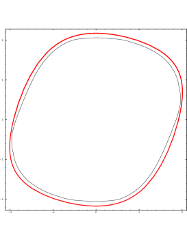
Figure 2: The limit cycle of the van der Pol equation (exterior curve) and the algebraic approximation $h_{18}(x,y)=K_{18}^{\star}$ .

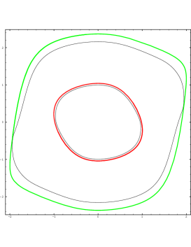
Figure 4: The limit cycles of equation (6) with $F(x)$ given by (11) (rough curves) and their algebraic approximations (smooth curves) : $h_{14}(x,y)=K_{14\,1}^{\star}$ and $h_{14}(x,y)=K_{14\,2}^{\star}$

Figure 5: We show, for the van der Pol equation, the curve $Log(K_{n}^{\star})$ in function of $n$

References

- [1] S. H. Strogatz, Nonlinear Dynamics and Chaos (Addison Wesley, 1994).
- [2] A. Nayfeh and B. Balachandran, Applied Nonlinear Dynamics (J. Wiley, New York, 1995).
- [3] L. Edelstein-Keshet, Mathematical Models in Biology (Random House, New York, 1988).
- [4] L. Salasnich, “Instabilities, Point Attractors and Limit Cycles in a Inflationary Universe”, Mod. Phys. Lett. A10, 3119 (1995).
- [5] D. Poland, “Loci of limit cycles”, Phys. Rev. E 49, 157 (1994).
- [6] L. Salasnich, “On the Limit Cycle of an Inflationary Universe”, Preprint Universita di Padova (1996).
- [7] Ye Yan-Qian et al., Theory of Limit Cycles, translations of mathematical monographs, Vol. 66 (American Mathematical Society, Providence, 1986).
- [8] R. Maier and D. Stein, “Oscillatory behaviour of the rate of escape through an unstable limit cycle”, Phys. Rev. Lett. 77, 4860 (1996).
- [9] M. Farkas, Periodic Motion (Springer, Berlin, 1994).
- [10] H.Giacomini and M.Viano, “Determination of limit cycles for two-dimensional dynamical systems”, Physical Review E 52, 222 (1995).
- [11] H. Giacomini, J. Llibre and M. Viano, “On the nonexistence, existence and uniqueness of limit cycles”, Nonlinearity 9, 501 (1996).
- [12] B. Delamotte, “A non pertubative method for solving differential equations and finding limit cycles”, Phys. Rev. Lett. 70, 3361 (1993).
- [13] J. Rayleigh, The Theory of Sound , New York, Dover (1945).
- [14] B. van der Pol, “Forced oscillations in a circuit with nonlinear resistance”, London, Edinburgh and Dublin Phil. Mag. 3, 65 (1927).
- [15] A. Liénard, “Etude des oscillations entretenues”, Rev. Gen. d’électricité, XXIII, 901 (1928).
- [16] N. Levinson and D. Smith, “A genereal equation for relaxation oscillations”, Duke Math. Journal 9, 382 (1942).
- [17] A. Lins, W. de Melo and C. Pugh, On Liénard’s equation, Lecture Notes in Mathematics 597, 335, Springer-Verlag (1977).
- [18] L. Perko, Differential Equations and Dynamical Systems (Springer-Verlag, second edition, 1996).
- [19] N.G. Lloyd, New Directions in Dynamical Systems, London Math. Soc. Lecture Note Series N.127, edited by T.Bedford and J. Swift (Cambridge University Press, 1988).
- [20] F. Dumortier and C. Rousseau, “Cubic Liénard equations with linear damping”, Nonlinearity 3, 1015 (1990).
- [21] F. Dumortier and C. Li, “On the uniqueness of limit cycles surrounding one or more singularities for Liénard equations”, Nonlinearity 9, 1489 (1996).
- [22] T.Blows and N.Lloyd, “The number of small amplitude limit cycles of Liénard equations”, Math. Proc. Cambridge Phil. Soc. 95 (1984), 751.
- [23] Xun-Cheng Huang, “Uniqueness of limit cycles of generalized Liénard systems and predator-prey systems”, J. Phys. A : Math. Gen. 21, L685 (1988).
- [24] Yang Kuang and H. Freedman, “Uniqueness of limit cycles in Gause-type models of predator-prey systems”, Math. Biosciences 88, 67 (1988).
- [25] G.S. Rychkov, “The maximal number of limit cycles of the system is equal to two”, Differential Equations 11, (1975), 301.