Lyapunov Exponent and the Solid-Fluid Phase Transition

Abstract

We study changes in the chaotic properties of a many-body system undergoing a solid-fluid phase transition. To do this, we compute the temperature dependence of the largest Lyapunov exponents $\lambda_{\mbox{max}}$ for both two- and three-dimensional periodic systems of $N$-particles for various densities. The particles interact through a soft-core potential. The two-dimensional system exhibits an apparent second-order phase transition as indicated by a $\lambda$-shaped peak in the specific heat. The first derivative of $\lambda_{\mbox{max}}$ with respect to the temperature shows a peak at the same temperature. The three-dimensional system shows jumps, in both system energy and $\lambda_{\mbox{max}}$, at the same temperature, suggesting a first-order phase transition. Relaxation phenomena in the phase-transition region are analyzed by using the local time averages.

I Introduction

Molecular dynamics (MD)[1] is a computer simulation methods which relates the macroscopic properties of matter to a microscopic description of the constituent particles’ motion. In MD simulations Newton’s equations of motion are solved. Then, the thermodynmic quantities of the system, such as pressure and temperature, are obtained as time averages of corresponding physical quantities. These time averages are fully equivalent to statistical ensemble averages obtained by using the Monte Carlo (MC) simulations. The dynamic method has been successfully applied to simulating not only the static equilibrium systems, but also those in nonequilibrium.

Since the pioneering work of Hoover et al.[2], many investigations of the chaotic properties of the many- particle systems have been carried out. Our own goal is to understand the relation between the irreversible macroscopic behavior of the atomic systems and the underlying microscopic theory with time-reversal symmetry. The MD simulation provides a plausible clue to solving this long-standing problem. The main point is that the motion of the particles in a many-particle system is Lyapunov unstable; that is, the phase trajectories starting from neighboring initial points separate from one another exponentially in time, while they explore only a restricted portion of phase space, forming a stable strange attractor.

The spectrum of Lyapunov exponents $\{\lambda_{1},\cdots,\lambda_{M}\}$ is a powerful tool for the analysis of the properties of chaotic systems[3]. Lyapunov exponents measure the averaged exponential rates of divergence or convergence of neighboring trajectories in phase space: the sum of the first $n$ Lyapunov exponents is defined by the exponential growth or shrinking rate of an $n$-dimensional phase-space volume. The resulting $\lambda_{i}(i=1,2,\cdots,M)$ are conventionally arranged in decreasing order. For chaotic systems the largest exponent, $\lambda_{1}$ (hereafter we will also denote it as $\lambda_{\mbox{max}}$) is positive, so that neighboring trajectories diverge exponentially. The Lyapunov dimension, following the conjecture of Kaplan and York[4], is a lower bound on the fractal dimension of the above mentioned strange attractor. Furthermore, the sum of all positive Lyapunov exponents defines the Kolmogorov entropy[5, 6].

The most peculiar property of the many-particle systems is that they can be in different phases. A system can undergo a phase transition from one to another phase when temperature or pressure is changed appropriately. Thus, it is interesting to see how the chaotic properties of a system change during these phase transitions. Qualitative differences in the shapes of the Lyapunov spectra for fluids and solids were described in Ref.[7]. Further studies, described in Ref.[8], covered a wide range of densities and temperatures, and led to the conclusion that the spectral shape does not uniquely determine the phase of the system. A more quantitative analysis was carried out in Ref.[9], where Lyapunov exponents for the correlated cell model[10], the Lorenz gas model[11] and the Lennard-Jones fluid were evaluated as a function of the density for various energies. In all the cases studied the $\lambda_{\mbox{max}}$ exhibited a maximum near the phase transition.

In this work we have the same interest. We study $D$-dimensional ($D$=2,3) equilibrium dense fluid models, where $N$-particles in a periodic box interacting with a soft-core repulsive potential. We evaluate $\lambda_{\mbox{max}}$ for these systems, as a function of the temperature, for various densities. In the two-dimensional case, a careful analysis of the specific heat, shows a $\lambda$-shaped peak, suggesting that the system undergoes a solid-fluid phase transition of the second order. Next, it is shown that the first derivative of $\lambda_{\mbox{max}}$ with respect to the temperature has a peak at the same temperature. In the three-dimensional case $D$=3, both the system energy and $\lambda_{\mbox{max}}$ show jumps at the same temperature, implying that the phase transition is first-order. Such a phase transition takes place over a somewhat wide range of temperature, where two phases coexist, so that the time avergages require a much longer time to converge. With the help of the local time averages we can analyze relaxation phenomena in the phase-transition region.

In the following section II, we briefly describe the dense-fluid model and the method for evaluating the Lyapunov exponents. The numerical results for a two-dimenional system with $N$=30 and a three-dimensional system with $N$=32 are then presented and analysed in Sec. III and IV. A conclusion follows.

II Model of Dense Fluids and Solids at Equilibrium

The microscopic dynamics of dense fluids and solids at equilibrium can be modeled by a Newtonian many-body system of $N$-particles in a periodic box. The particles interact with each other through a short-range repulsive pair potential. In this work, to optimize the numerical processes, we adopt the short-range pair potential introduced in Ref.[2],

$$\phi=100(1-r^{2})^{4},\hskip 14.22636ptr<1,$$ (1)

truncated at the cutoff radius, $r=1$, where the first three derivatives vanish. The smooth truncation at short range minimizes the errors associated with numerical integration[2]. The repulsive part of this potential resembles that of the rare-gas system. The fact that the potential is finite at the origin does not cause any problem within the range of the system energy and density considered here. One may elaborate the model by employing a more realistic potential at the expense of additional notational complexity and reduced computing speed.

By choosing the side length $L$ of the periodic box larger than twice the interaction range, the problem becomes relatively simple. Among all the possible pairs of particle $i$ and particle $j$, with its imaginary periodic particles $j^{\prime}$, only the one with the shortest separation distance can be included in evaluating the potential energy.

Let ${\mathchoice{{\hbox{\boldmath$\displaystyle\Gamma$}}}{{\hbox{\boldmath$\textstyle\Gamma$}}}{{\hbox{\boldmath$\scriptstyle\Gamma$}}}{{\hbox{\boldmath$\scriptscriptstyle\Gamma$}}}}(t)$ be the phase space vector of $2DN$ variables describing the motion of the particles

$$\mathchoice{{\hbox{\boldmath$\displaystyle\Gamma$}}}{{\hbox{\boldmath$\textstyle\Gamma$}}}{{\hbox{\boldmath$\scriptstyle\Gamma$}}}{{\hbox{\boldmath$\scriptscriptstyle\Gamma$}}}(t)\equiv(x_{1},x_{2},\cdots,x_{N},y_{1},\cdots,z_{N};p_{x_{1}},\cdots,p_{z_{N}}).$$ (2)

One may reduce the dimension of the phase-space vector by using the fact that the center-of-mass motion of the system is trivial and further by using the energy conservation. However, implementing this idea involves a lot of unnecessary complication.

The Hamiltonian for the particle system is expressed as

$$H=\sum_{i=1}^{N}\textstyle\frac{1}{2}p_{i}^{2}+\displaystyle\sum_{i>j}\phi(r_{ij})$$ (3)

where $r_{ij}$ is the shortest distance between particle $i$ and particle $j$, $j^{\prime}$, $\cdots$ as explained above. Note that the summation for the potential energy is not restricted to the pair potential between particles within the system box, including image particles. The Hamiltonian equations of motion

$$\dot{q}=\frac{\partial H}{\partial p},\hskip 20.00003pt\dot{p}=-\frac{\partial H}{\partial q}$$ (4)

lead to a set of the first-order differential equations expressed in a form of

$$\dot{\mathchoice{{\hbox{\boldmath$\displaystyle\Gamma$}}}{{\hbox{\boldmath$\textstyle\Gamma$}}}{{\hbox{\boldmath$\scriptstyle\Gamma$}}}{{\hbox{\boldmath$\scriptscriptstyle\Gamma$}}}}={\mathchoice{{\hbox{\boldmath$\displaystyle G$}}}{{\hbox{\boldmath$\textstyle G$}}}{{\hbox{\boldmath$\scriptstyle G$}}}{{\hbox{\boldmath$\scriptscriptstyle G$}}}}({\mathchoice{{\hbox{\boldmath$\displaystyle\Gamma$}}}{{\hbox{\boldmath$\textstyle\Gamma$}}}{{\hbox{\boldmath$\scriptstyle\Gamma$}}}{{\hbox{\boldmath$\scriptscriptstyle\Gamma$}}}}).$$ (5)

These equations describe the microscopic dynamics of the system in phase-space. The macroscopic properties of the system can be studied through the thermodynamical quantities defined by time averages. For example, the temperature of the system is defined as

$$\frac{D}{2}NT\equiv\langle\sum_{i=1}^{N}\textstyle\frac{1}{2}p^{2}_{i}\rangle_{t}=\displaystyle\lim_{\tau\rightarrow\infty}\int^{\tau}_{0}\!\!\!dt\sum_{i=1}^{N}\textstyle\frac{1}{2}p_{i}^{2}.$$ (6)

Here, we use reduced units for which the mass of the particle, the interaction range of the potential, and Boltzmann’s constant are unity.

Lyapunov exponents $(\lambda_{1}$, $\lambda_{2}$, $\cdots)$ measure the long-term averaged exponential rates of divergence or convergence of neighboring trajectories in phase space. They are arranged in decreasing order, the first (largest) Lyapunov exponent, $\lambda_{1}$ (equivalently denoted as $\lambda_{\mbox{max}}$ throughout this paper), describes the exponential growth rate of the distance ($\ell_{1}$) between the reference trajectory and the satellite trajectory 1, the sum of the first two, $\lambda_{1}+\lambda_{2}$, describes that of the area $(a_{12})$ spanned by the reference trajectory and the two satellite trajectories 1 and 2, and so on. In this paper, we will consider only the largest exponent $\lambda_{\mbox{max}}$. It can be calculated by monitoring the length of a differential offset vector $\delta\mathchoice{{\hbox{\boldmath$\displaystyle\Gamma$}}}{{\hbox{\boldmath$\textstyle\Gamma$}}}{{\hbox{\boldmath$\scriptstyle\Gamma$}}}{{\hbox{\boldmath$\scriptscriptstyle\Gamma$}}}$ in the tanget space to the reference trajectory. It presents a satelite trajectory infinitesimally separated from the reference one, with equations of motion derived from Eq.(5) in a linearized form:

$$\delta\dot{\mathchoice{{\hbox{\boldmath$\displaystyle\Gamma$}}}{{\hbox{\boldmath$\textstyle\Gamma$}}}{{\hbox{\boldmath$\scriptstyle\Gamma$}}}{{\hbox{\boldmath$\scriptscriptstyle\Gamma$}}}}=\frac{\partial\mathchoice{{\hbox{\boldmath$\displaystyle G$}}}{{\hbox{\boldmath$\textstyle G$}}}{{\hbox{\boldmath$\scriptstyle G$}}}{{\hbox{\boldmath$\scriptscriptstyle G$}}}}{\partial\mathchoice{{\hbox{\boldmath$\displaystyle\Gamma$}}}{{\hbox{\boldmath$\textstyle\Gamma$}}}{{\hbox{\boldmath$\scriptstyle\Gamma$}}}{{\hbox{\boldmath$\scriptscriptstyle\Gamma$}}}}\cdot\delta\mathchoice{{\hbox{\boldmath$\displaystyle\Gamma$}}}{{\hbox{\boldmath$\textstyle\Gamma$}}}{{\hbox{\boldmath$\scriptstyle\Gamma$}}}{{\hbox{\boldmath$\scriptscriptstyle\Gamma$}}}$$ (7)

III Two-Dimensional System

We consider here a system of $N$=30 interacting particles moving in a rectangular periodic box. The size and the shape of the periodic box is chosen to contain $15(=5\times 3)$ primitive cells of the triangular lattice when the particles are arranged into a configuration of the lowest potential energy. (See Fig. 1a.) Finite-size effects are minimized by using the periodic boundary condition. Since the dimension of the primitive cell containing two particles is $d\times\sqrt{3}d$ with the lattice constant $d$, the particle number density $\rho$ is determined as $\rho=2/(\sqrt{3}d^{2})$ and the shape of the periodic box is close to a square (i.e., $L_{x}:L_{y}=5:3\sqrt{3}$). At $t$=0, 30 particles begin to move from a triangular lattice configuration, which is denoted by the solid circles in Fig. 1. For $\rho>2/\sqrt{3}\sim 1.15$, six nearest neighboring particles can be found within the interaction range. It leads to a nonvanishing potential energy of $V_{0}=\phi(d)\times 6\times 30\times\frac{1}{2}$. In the following discussions, for a convenience we will subtract $V_{0}$ from the total energy of the system. The velocities of the particles are chosen randomly with a fixed total kinetic energy which determines the total energy $E$. Then, the equations of motion are solved numerically, using fourth-order Runge-Kutta method with the time step 0.001. This time step 0.001 is sufficiently small for all temperatures and densities studied in this work: the total energy is conserved with an accuracy of at least eight decimal digits.

In Fig. 1, we show two characteristic motions of a single particle in a two-dimensional system of density $\rho=1.2$ at different system energies $E/N=0.01$ and $E/N=1.5$. We present the trajectories of a single particle for the first 100 time units after the particles begin to move. In case of $E/N=0.01$ (Fig.1a), each particle moves in a restricted area around its initial position. Such motion defines a solid phase, where the system maintains an ordered configuration. On the other hand, in the system with $E/N=1.5$(Fig. 1b) a particle can wander over the all the space with no restriction, defining the fluid phase. The system may exhibit other phases such as gas or glass. In any cases, there should be certain temperature(s) the system transfers from one phase to another.

Our interest here is relating the phase transition to the chaoticity of a system changing due to such a phase transition. In Fig. 2, we present numerical results for the time-averaged kinetic energy per particle ($\langle K\rangle/N$ = temperature $T$) versus the total energy per particle and the largest Lyapunov exponent versus the temperature for the systems at two different densities. For each density, we carry out 80 simulations at every $E/N=0.05$ up to $E/N=4.0$. Open circles denote time averages taken over 2000 time units ($\tau=2000$), excluding data up to first 100 time units. To corroborate convergence, we present time averages evaluated for $\tau=1000$ by the filled circles. As for the time-averaged kinetic energies, the convergence is quite good. The filled circles can be hardly seen behind the open circles due to their small differences. We interpret the difference between them as a relative error of the numerical calculation. The temperatures are obtained with 0.1% accuracy. The Lyapunov exponents converge rather slowly. Compared with the averages of $\tau=1000$, those of $\tau=2000$ reveal relative errors up to 1%.

The data do not seem to exhibit any sudden changes indicating a phase transition. In case of $\rho=1.0$, the system energy per particle $E/N$ is almost linear in temperature $T$ and $\lambda_{\mbox{max}}$ can be fitted by a single curve of

$$\lambda_{\mbox{max}}=\alpha T^{\beta},$$ (8)

with $\beta\sim 0.38$. The data for the system of $\rho=1.2$ show similar dependences on temperature. Only a small deviation in $\lambda_{\mbox{max}}$ curve from the power function of Eq.(8) (with $\beta=0.43$) can be noticed over a wide range of $0.2\,\raisebox{-2.15277pt}{$\stackrel{{\scriptstyle\textstyle<}}{{\sim}}$}\,T\,\raisebox{-2.15277pt}{$\stackrel{{\scriptstyle\textstyle<}}{{\sim}}$}\,0.7$.

Such a smooth dependence of $E/N$ on temperature may imply that there is no phase transition at all or, if any, that it is of higher than first order. To investigate further we considered the specific heat defined as

$$C_{V}\equiv\frac{d(E/N)}{dT},$$ (9)

and the first derivative of $\lambda_{\mbox{max}}$ with respect to temperature $d\lambda_{\mbox{max}}/dT$. From the obtained data for $E/N$ versus $T$ and $\lambda_{\mbox{max}}$ versus $T$, the derivatives can be evaluated numerically, for example, by using the Lagrange’s three-point interpolation formula.

In Fig. 3, the resulting derivatives are presented as a function of the temperature for the system of $\rho=1.0$. We have used three data points with $\Delta(E/N)=0.15$ throughout. The error bars in the figures were estimated by comparing the results of $\tau=1000$ and $\tau=2000$ as mentioned above. In Fig. 3(a), for all the temperatures the specific heat has almost a constant value ($\sim 1.45$), which is larger than that of the two-dimensional ideal gas ($C_{V}/N=1$) but smaller than that of the ideal solid ($C_{V}/N=2$). The temperature dependence of $d\lambda_{\mbox{max}}/dT$ is trivial; it decreases monotonically as temperature increases. We conclude that in case of $\rho=1.0$ the system stays in a single phase, for all the temperatrures in the range studied.

Fig. 4(a) and (b), respectively, are the specific heat and $d\lambda_{\mbox{max}}/dT$ for the system of $\rho=1.2$. The specific heat exhibits a $\lambda$-shaped peak around $T\sim.56$. The first derivative, $d\lambda_{\mbox{max}}/dT$, shows also a peak at the same temperature on top of the monotonically decreasing background curve. Although the finite-size effects and the large $\Delta T$ used in the numerical differentiation would have made the shapes of the peaks less sharp, those peaks are sufficiently well-defined to support our conclusion that the system undergoes a solid-fluid phase transition of the second-order at the corresponding temperature.

IV Three-Dimensional System

The three-dimensional system studied here is $N$=32 interacting particles moving in a periodic cubic box. The periodic box contains $8(=2\times 2\times 2)$ primitive cells of the face-centered-cubic(fcc) lattice when the particles are in the configuration of the minimum potential energy. Since the volume of the cubic primitive cell containing four particles is $(\sqrt{2}d)^{3}$ with the lattice constant $d$, the particle number density $\rho$ is determined simply as $\rho=\sqrt{2}/d^{3}$.

In Fig. 5, the same quantities studied in Sec. IV (that is, $E/N$, $\lambda_{\mbox{max}}$ and their derivatives with respect to the temperature) are presented as a function of the temperature for the three-dimensional system with particle density $\rho=1.0$. The temperature is now defined as $T\equiv\frac{3}{2}(\langle K\rangle/N)$. The averages are also taken for $\tau=2000$ after discarding data from the initial time interval of length $t=100$. At this density, the system energy per particle $E/N$ shows a trivial linear dependence on the temperature (Fig. 5a), which leads to almost constant specific heat (Fig. 5c). The temperature dependence of $\lambda_{\mbox{max}}$ can be fitted into a power function of Eq.(8) with $\beta=0.37$. These facts suggest that the system of $\rho=1.2$ remains in a single phase, i.e., the fluid phase.

Fig. 6 are show $E/N$ versus $T$ and $\lambda_{\mbox{max}}$ versus $T$ for the systems of the particle density $\rho=1.3$(a,c) and $\rho=1.4$(b,d). In case of $\rho=1.3$, discrete jumps can be seen both in the $E/N$ versus $T$ graph and in the $\lambda_{\mbox{max}}$ versus $T$ graph at the same temperature $T\sim 0.14$. Note that this already happens below $\rho_{c}=\sqrt{2}$, at which density the particles begin to contact each other in the minimum energy fcc configuration. (The subcript ‘c’ refers to ‘contact’.) A similar discrete jump can be seen also in the system with $\rho=1.4$ at higher temperature. Furthermore, over a wide range of temperature ($0.26\,\raisebox{-2.15277pt}{$\stackrel{{\scriptstyle\textstyle<}}{{\sim}}$}\,T\,\raisebox{-2.15277pt}{$\stackrel{{\scriptstyle\textstyle<}}{{\sim}}$}\,0.32$. the averages taken over $\tau=2000$ show large deviations from those over $\tau=1000$.

Such poor convergence of the averages indicates that the system is unstable near the phase transition. In Fig. 7, we present the average values $T(\equiv\frac{2}{3}\langle K\rangle/N)$ and $\lambda_{\mbox{max}}$ as a function of $\tau$ over which the averages are taken. The dashed-dotted curves are averages for the system of $E/N=0.5$ which show a good convergence to stable constant values. Especially, the convergence of the averaged kinetic energy is remarkably rapid compared to the Lyapunov exponent. Such a standard behavior holds for all the averages that have been discussed up to now. Furthermore, the resulting averages do not depend on the initial conditions. On the other hand, the solid curves are the averages for the system of $E/N=0.7$. The averages seem to reach somewhat stable values up to $\tau\sim 600$, at which point the averages suddenly depart from those trends. They also show a strong dependence on the initial conditions of the simulations. The dashed curves are the corresponding quantities for the system of the same energy $E/N=0.7$ but started from different set of initial velocities. At first, the averages tends to converge to different values from those of the solid curves till the sudden changes occur again. The final values of the solid and dashed curves at $\tau=2000$ seem to converge to the same value but they still show a large difference.

In order to understand such a peculiar behavior in taking the averages, we introduce ‘local’ averages in the vicinity of $t$ defined as

$$\langle A\rangle(t)\equiv\frac{1}{\Delta\tau}\int^{t+\frac{1}{2}\Delta\tau}_{t-\frac{1}{2}\Delta\tau}dt^{\prime}A(t^{\prime}).$$ (10)

In Fig. 8, shown are the local temperature and Lyapunov exponents that lead to the accumulated averages shown in Fig.7 (solid and dash-dotted curves). The local averages for the system of $E/N=0.5$ oscillate about a single value, resulting in a stable cumulative average. In case of $E/N=0.7$, there appear instead to be two centers of oscillation for the local averages, indicating that the system has two ‘quasi-stable’ phases. The system cannot stay in either phase but instead changes between the phases from time to time. Note that the transfer occurs abruptly because the system is relatively small.

How long the system stays in one phase is senstive to initial conditions; that is, a tiny difference in the initial conditions or any small fluctuations coming from roundoff errors in the numerical simulations leads to quite different results. This interpretation explains not only the abrupt changes in the accumulated averages in Fig. 7 but also the strong dependence of them on the initial conditions. Thus, in order to obtain averages with a few-digit accuracy we have to simulate the motion for a large $\tau$ in the phase-transition region. Shown in Fig. 9 are the distributions of local averages obtained with $\Delta\tau=5$ for 20000 time units (ten times longer than what we have used in evaluating the averages discussed so far). In case of $E/N=0.5$ the distribution of the local temperature and the local Lyapunov exponents (black bars) can be fitted into single Gaussian curves (solid lines). On the other hand, those for the system in the phase transition region($E/N=0.7$, white bars) split into two Gaussian distributions. The dashed ones are the separate Gaussian curves and the solid one is their sum, which fits the whole distributions. Those two Gaussian curves correspond to the quasistable fluid and solid phases of the system, respectively.

By noticing that the two Gaussian curves for the distribution of the local temperature is clearly divided into two, we can evaluate the averages of the quasi-stable phases separately. To do this, we sum up the local temperature and local Lyapunov exponents for the time period when $T_{\mbox{local}}<T_{\mbox{sep.}}$ or $T_{\mbox{local}}>T_{\mbox{sep.}}$ with a properly chosen $T_{\mbox{sep.}}$. (See Fig.9 for the definition of $T_{\mbox{sep.}}$.) The genuine overall average of the system lies in between those two values. Shown in Fig.10 are those averages of the system obtained through a similar analysis with the local averages for $\tau=20000$; that is, the overall averages (solid circles) and the averages of the quasistable phases (open circles). The error bars for the solid circles indicate the standard deviations of the local averages. The quasistable phases smoothly match with the averages of the system in a stable single phase. Thus, those quasi-stable phases can be interpreted as the “super-cooled” fluid phase and “super-heated” solid phase in the literature. The $E/N$ versus $T$ data for the quasi-stable phases and the stable single phase can be fit into a straight line, $E/N=2.87T-0.09$ for the solid phase and $E/N=2.90T+0.08$ for the fluid phase around the phase transition region. It enables us to evaluate the latent heat (per particle) associated with the phase transition as $\Delta\ell\sim 0.17(=0.08+0.09)$. Mixing phenomena in the hard sphere system have been investigated by using the maximum Lyapunov exponents in Ref.[14].

Although the data we obtained still show large standard deviations, they are sufficiently precise for us to see what happens in our 3-dimensional system when it undergoes a phase transition. That is, our three-dimensional system undergoes a first-order phase transition. The system energy and the largest Lyapunov exponent discontinuously jump at the temperature of the phase transition.

V Conclusions

In this work, we studied changes in the chaos of a many-body system as that system underwent a phase transition. As models we considered $N$-particles moving in two-dimensional ($N=30$) or three-dimensional ($N=32$) periodic boxes. The particles interacted with each other through a short-ranged repulsive potential with a soft-core. We computed the largest Lyapunov exponents for the motions of the particles as a function of temperature for a few different densities. Relaxation phenomena in the phase transition region were analyzed by using the local time averages. In a conclusion, the Lyapunov exponent can be a good physical quantity for investigating the phase transition. It may tell us when the phase transition occurs and what kind of phase transition is involved.

Here we have considered only a simple soft-core potential only with the repulsive interactions. Furthermore, we have carried out the simulation with a fixed system energy. To see whether or not the difference in transition order is more general, we will have to check it carefully for the other systems with more realistic interactions and/or for the thermostatted systems with a fixed temperature. Work in this direction is under progress and will be reported elsewhere[15].

FIG. 1.: Two characteristic single-particle motions of the system (a) in the solid phase and (b) in the fluid phase.

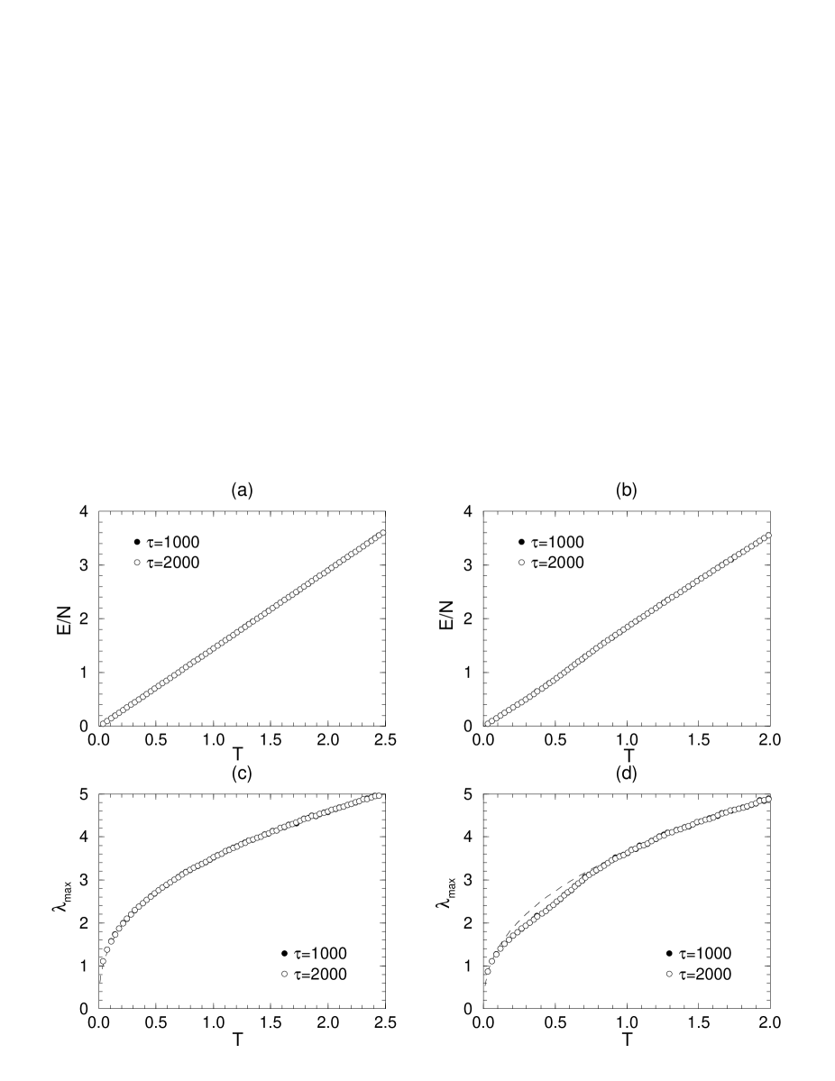
FIG. 2.: $E/N$ versus temperature($T$) and $\lambda_{\mbox{max}}$ versus T for the system with $\rho=1.0$ (a,b) and $\rho=1.2$ (c,d).

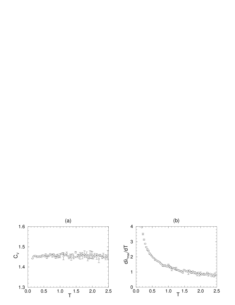
FIG. 3.: The specific $C_{V}$ and $d\lambda_{\mbox{max}}/dT$ versus temperature for the system of $\rho=1.0$.

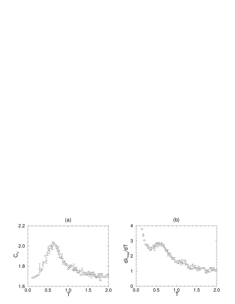
FIG. 4.: Same quantities as Fig. 3 for the system of $\rho=1.2$.

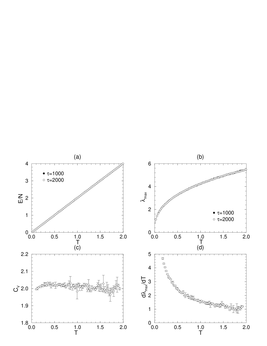
FIG. 5.: (a) $E/N$ versus temperature($T$), (b) $\lambda_{\mbox{max}}$ versus $T$, (c) $C_{V}$ versus $T$, and (d) $d\lambda_{\mbox{max}}/dT$ versus T for a three-dimensional system with the particle density $\rho=1.0$.

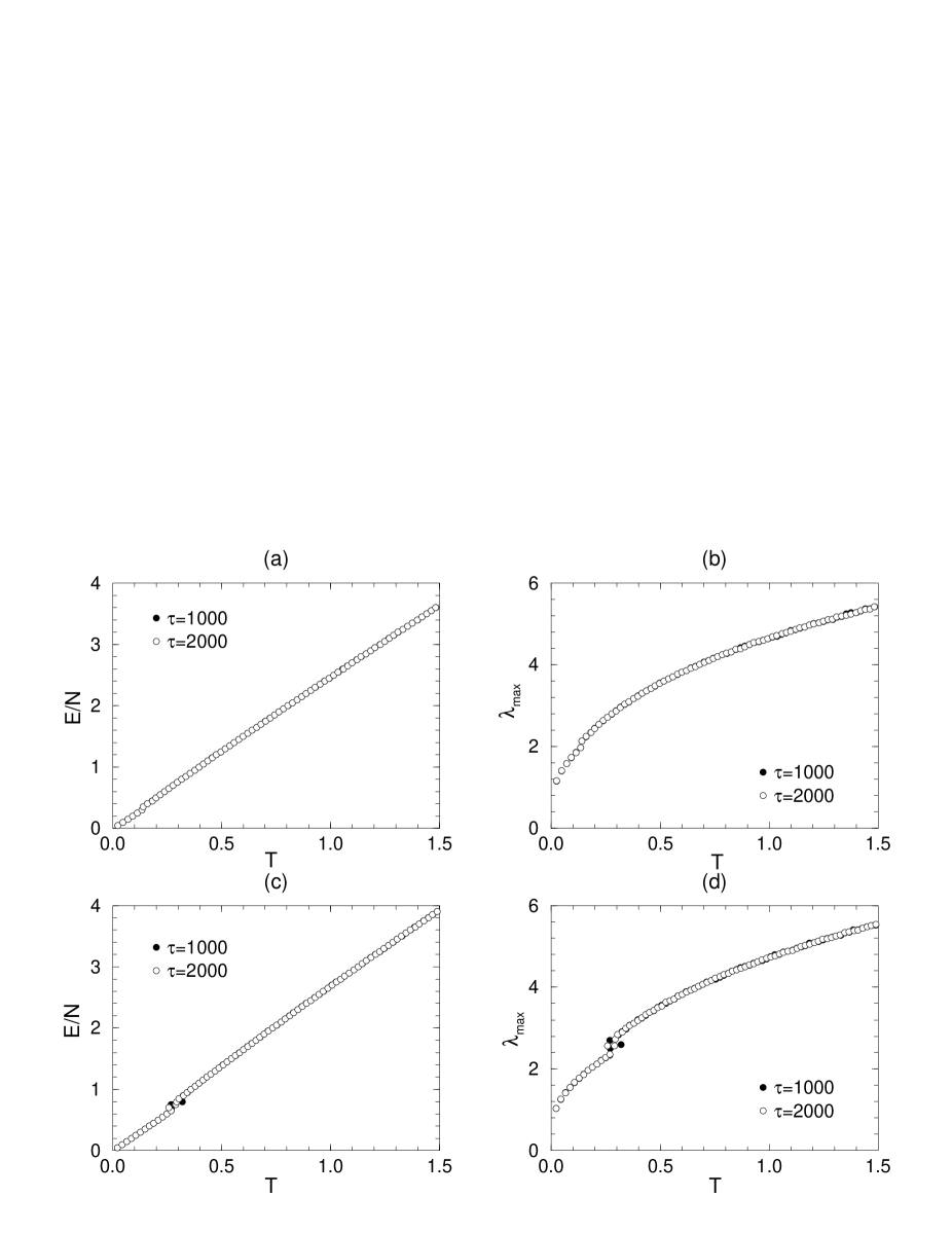
FIG. 6.: (a) $E/N$ versus temperature($T$), (b) $\lambda_{\mbox{max}}$ versus $T$ for the system of particle density $\rho=1.3$, and (c) $E/N$ versus $T$, and (d) $\lambda_{\mbox{max}}$ versus T for the system with $\rho=1.4$.

FIG. 7.: Poor convergence of averages near the phase transition : (a) $T(\equiv\frac{3}{2}\langle K\rangle/N)$ and (b) $\lambda_{\mbox{max}}$ as a function of $\tau$ for the system of $\rho=1.4$ with $E/N=0.7$ (solid lines). The dash-dotted lines are the corresponding averages for the system of the same particle density but with $E/N=0.5$, which converge rapidly to stable values.

FIG. 8.: Local averages with $\Delta\tau=5$ for the system of density $\rho=1.4$ and energy $E/N=0.5$ and 0.7 : (a) $T(\equiv\frac{3}{2}\langle K\rangle/N)$ and (b) $\lambda_{\mbox{max}}$.

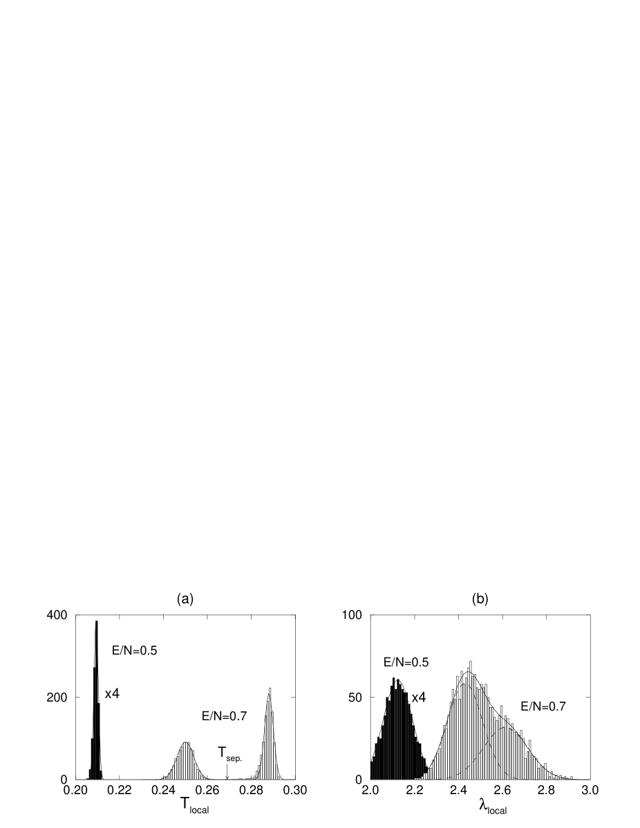
FIG. 9.: Distribution of local averages with $\Delta\tau=5$ for $\tau=20000$ for the system of density $\rho=1.4$ and energy $E/N=0.5$ and 0.7 : (a) $T(\equiv\frac{3}{2}\langle K\rangle/N)$ and (b) $\lambda_{\mbox{max}}$.

FIG. 10.: (a) $E/N$ versus $T$ and (b) $\lambda_{\mbox{max}}$ versus $T$ near the phase transition. The solid circles are the overall accumulated averages of the system for $\tau=20000$ and the open circles are averages of the quasi-stable phases obtained in the way described in the text.

- [1] For an introduction, see W. G. Hoover, Computational Statistical Mechanics (Elsevier, Amsterdam, 1991).
- [2] W. G. Hoover, H. A. Posch, and S. Bestiale, J. Chem. Phys. 87 6665 (1987); H. A. Posch and W. G. Hoover, Phys. Rev. A38, 473 (1988).
- [3] For a review, see A. Wolf, J. B. Swift, H. L. Swinney, and A. Vastano, Physica 16D, 285 (1985); J-P. Eckmann and D. Ruelle, Rev. Mod. Phys. 57, 617 (1985).
- [4] J. Kaplan and J. Yorke, in Fundamental Differential Equations and the Approximation of Fixed Points, Vol. 730 of Lecture Notes in Mathematics, edited by H. O. Peitgen and H. O. Walther (Springer-Verlag, Berlin, 1978).
- [5] G. Benettin, L. Galgani, and J. Strelcyn, Phys. Rev. A14, 2338 (1976).
- [6] I. Shimada and T. Nagashima, Prog. Theor. Phys. 61, 1605 (1979).
- [7] H. A. Posch and W. G. Hoover, Phys. Rev. A39, 2175 (1989).
- [8] I. Borzák, A. Baranyai and H. A. Posch, Physica A229, 93 (1996).
- [9] Ch. Dellago and H. A. Posch, Physica A230, 364 (1996).
- [10] B. J. Alder, W. G. Hoover and T. E. Wainwright, Phys. Rev. Lett. 11, 241 (1963).
- [11] J. Machta and R. Zwanzig, Phys. Rev. Lett. 50, 1959 (1983).
- [12] G. Benettin, L. Galgani, A. Giorgilli, and J. M. Strelcyn, C. R. Acad. Sci.(Paris) 286A, 431 (1978); Mechanica 15, 9 (1978).
- [13] W. G. Hoover and H. A. Posch, Phys. Lett. A113, 82 (1985).
- [14] Ch. Dellago and H. A. Posch, Phys. Rev. E55, R9 (1997).
- [15] K.-H. Kwon and B.-Y. Park, work in progress.