Quantum chaotic attractor in a dissipative system

Abstract

A dissipative quantum system is treated here by coupling it with a heat bath of harmonic oscillators. Through quantum Langevin equations and Ehrenfest’s theorem, we establish explicitly the quantum Duffing equations with a double-well potential chosen. A quantum noise term appears the only driving force in dynamics. Numerical studies show that the chaotic attractor exists in this system while chaos is certainly forbidden in the classical counterpart.

Quantum chaos of Hamiltonian systems has been studied extensively [1, 2, 3, 4]. By contrast, very little work has been done in looking at quantum chaos of dissipative systems. Many quantum mechanical systems (e.g., SQUID with Josephson junction, an atom in a cavity of electromagnetic fields, NMR quantum measurements), however, are neither isolated nor Hamiltonian. These interact with their environment and thus are open in general and noisy and dissipative. Dissipation is relatively difficult to treat in a quantum system since it seems inevitable to deal with stochastic processes via, for instance, the commonly used master equation that is extremely difficult to solve numerically. Recently, Spiller and Ralph [5] studied a damped and driven non-linear oscillator by using the quantum state diffusion model based on the assumed master equation of Lindblad form [6]. They simulated the behavior of one member of the ensemble with a single environment operator and found that the quantum noise “kicks” the motion between the chaotic and the periodic behavior and so smears out any fractal structure. In general, the quantum state diffusion method often demands an approximation of the effects of the complicated environment by simple operators and always has a problem regarding the dimension of the environment [7]. Brun [8] has tried to derive the quantum version of the forced and damped Duffing oscillator through the decoherence approach which involves the path integral. As he noticed, performing calculations in the low-temperature limit is extremely difficult. For the high temperature limit, Brun also suggested that the quantum noise “smears out” the quantum maps based on Wigner distributions and that numerical computation cannot be efficiently done because of the necessity of enumerating all the possible histories and elements of the decoherence functional.

The dissipative quantum system has been studied by means of several different theories, for instance, the influence functional approach of Feynman and Vernon [9] and its application to Brownian motion [10], the quantum Langevin equations [11], the master equations [5, 6, 7, 11], etc. [12]. Among these, the quantum Langevin formalism is more interesting for us since the dynamics of quantum operators for the system can be explicitly given in a fashion quite similar to the classical one. Most of above theories considered a generic model of the system-bath interaction. Recently, Pattanayak and Schieve [3] proposed a derivation of semiclassical dynamics directly from Heisenberg equations of motion via Ehrenfest’s theorem where ostensible (apparent) quantum chaos was found for the conservative (Hamiltonian) system with a double-well potential. In this paper, we will study a dissipative quantum model similar to that of Refs. [9, 10, 11] and write explicitly the quantum Duffing equations for a system of double-well potential by means of Langevin formalism and Ehrenfest’s theorem. Numerical results are now possible to obtain and show that chaotic attractors robustly exist in this model whereas chaos is impossible for the corresponding classical Duffing system due to the absence of an external driving force.

To do this, let us consider a particle of unit mass moving in a one-dimensional time-independent bounded potential $V(\hat{Q})$ with its Hamiltonian, $H_{sys}={1\over 2}\hat{P}^{2}+V(\hat{Q}).$ To introduce dissipation, we may take the system $H_{sys}$ linearly interacting with an external “heat bath” of many degrees of freedom, which here is assumed an assembly of harmonic oscillators [9, 10, 11]. The familiar example of this model is a system of an atom interacting with a bath of equilibrium photons. Then the complete Hamiltonian is [9, 10, 11],

$$H = {\hat{P}^{2}\over 2}+V(\hat{Q})+\sum_{n}\left\{{\hat{p}_{n}^{2}\over 2m}+{1\over 2}m\omega_{n}^{2}(\hat{x}_{n}-{C_{n}\hat{Q}\over m\omega_{n}^{2}})^{2}\right\},$$ (1)

in which we have assumed that all harmonic oscillators possess the same mass $m$ but may have different frequency $\omega_{n}$ and that $C_{n}$ is the coupling constant between the system and the $n$th oscillator. The equal times commutation relations implicit in (1) are ${[\hat{Q},\hat{P}]}=i\hbar,{[\hat{Q},\hat{x}_{n}]}={[\hat{Q},\hat{p}_{n}]}=[\hat{P},\hat{x}_{n}]=[\hat{P},\hat{p}_{n}]=0,{[\hat{x}_{l},\hat{x}_{n}]}=[\hat{p}_{l},\hat{p}_{n}]=0$ and ${[\hat{x}_{l},\hat{p}_{n}]=i\hbar\delta_{ln}}$. Now it is straightforward to write down the Heisenberg equations of motion for the complete system. Then we may apply the standard procedure of Ref. [11] to derive the quantum Langevin equations. Assuming a continuous frequency distribution $g(\omega)$ of harmonic oscillators and using the first Markov approximation

$${g(\omega){C}^{2}(\omega)\over m\omega^{2}}\equiv{2\gamma\over\pi}$$ (2)

where $\gamma$ is assumed constant, we then have

$$\dot{\hat{Q}} = \hat{P},$$ (4)

$$\dot{\hat{P}} = -V^{\prime}(\hat{Q})-\gamma\hat{P}+\hat{\xi}(t),$$ (5)

where $\hat{\xi}(t)$ is the quantum noise operator due to the heat bath and $\gamma$ defined by (2) clearly represents the constant damping coefficient. Suppose that the system and the bath are initially independent (at $t\rightarrow-\infty$) so that the complete density operator can be written into $\rho=\rho_{sys}\otimes\rho_{b}$, and that the bath is initially thermal, $\rho_{b}\sim\exp(-H_{b}/k_{B}T)$. Then, $\hat{\xi}(t)$ has the properties (see, for example, [11])

$$\langle\hat{\xi}(t)\rangle = 0,$$ (7)

$$\langle[\hat{\xi}(t^{\prime}),\hat{\xi}(t)]_{+}\rangle = {2\gamma\hbar\over\pi}\int_{0}^{\infty}d\omega\omega\coth({\hbar\omega\over 2k_{B}T})\cos\omega(t^{\prime}-t),$$ (8)

in which $[\cdots]_{+}$ denotes an anticommutator. The average $\langle\cdots\rangle$ is over all bath variables. The operator nature of $\hat{\xi}(t)$ can be reduced by using the strategy of the adjoint commutative representation [13]. We can define a new operator $\eta(t)$ by $\eta(t)\rho(t^{\prime})\equiv{1\over 2}[\hat{\xi}(t),\rho(t^{\prime})]_{+}$ for all $t$ and $t^{\prime}$, which yields $[\eta(t),\eta(t^{\prime})]=0$. This means that $\eta(t)$ is a $c$-number function of time. Let us replace the operator $\hat{\xi}(t)$ by the $c$-number $\eta(t)$ in (2). Its $1$- and $2$-point correlation functions are given by (Quantum chaotic attractor in a dissipative system). In the following we will restrict ourselves in low temperature limit (not discussed in [8]), $T\rightarrow 0$, in which quantum effects are most important. In this limit the noise $\eta(t)$ is given by

$$\langle\eta(t)\rangle = 0,$$ (10)

$$\langle\eta(t)\eta(t^{\prime})\rangle = {\gamma\hbar\over\pi}\int_{0}^{\infty}d\omega\omega\cos\omega(t^{\prime}-t)$$ (11)

$$= -{\gamma\hbar\over\pi}{1\over(t-t^{\prime})^{2}}.$$ (12)

To obtain this, an exponential cutoff ($e^{-\epsilon\omega}$) was used, letting $\epsilon\rightarrow 0$ after integration [14].

While the dependence of bath operators has been eliminated in it, the quantum Langevin equations (2) are still operator equations and are as difficult as that in the deterministic quantum mechanics. To make further progress, we make an additional assumption that the wave packet of the system can be described by the squeezed coherent state [15]. Then we have the relations [3] $\langle\tilde{Q}^{2m}\rangle=(2m)!(\hbar\mu)^{m}/m!2^{m},\langle\tilde{Q}^{2m+1}\rangle=0,\langle\tilde{P}^{2}\rangle=\hbar(1+\alpha^{2})/4\mu,\langle\tilde{Q}\tilde{P}+\tilde{P}\tilde{Q}\rangle=\hbar\alpha,$ where $\tilde{O}{=}\hat{O}-\langle\hat{O}\rangle$ henceforth and $\langle\cdots\rangle$ denotes the expectation value. It has been shown that these are exactly equivalent to those derived from the generalized Gaussian wave functions [16, 17, 18]. The equations of motion for the centroid of a wave packet representing the particle are given from (2) by

$$\langle\dot{\hat{Q}}\rangle = \langle\hat{P}\rangle,$$ (14)

$$\langle\dot{\hat{P}}\rangle = -\langle V^{\prime}(\hat{Q})\rangle-\gamma\langle\hat{P}\rangle+\eta(t).$$ (15)

We now expand the equations around the centroid by using the identity $F(\hat{Q})=\sum_{n}F^{(n)}\tilde{Q}^{n}/n!$, where $F^{(n)}=\partial^{n}F(\hat{Q})/\partial\hat{Q}^{n}|_{\hat{Q}=\langle\hat{Q}\rangle}$, and for a double-well potential of $V(\hat{Q})=-{1\over 2}a\hat{Q}^{2}+{1\over 4}b\hat{Q}^{4}$ obtain the closed system of the stochastic differential equations

$$\dot{Q} = P,$$ (17)

$$\dot{P} = aQ-bQ^{3}-3bQ\hbar\mu-\gamma P+\eta(t),$$ (18)

$$\dot{\mu} = \alpha,$$ (19)

$$\dot{\alpha} = {1+\alpha^{2}\over 2\mu}+2\mu(a-3bQ^{2})-6b\hbar\mu^{2}-\gamma\alpha.$$ (20)

Here we have written $Q,P$ for $\langle\hat{Q}\rangle,\langle\hat{P}\rangle$. We remind the reader that all physical observables must be obtained by averaging over stochastic noise $\eta(t)$. When damping constant $\gamma$ is set to zero, the system is Hamiltonian with $H_{extended}={P^{2}\over 2}+{\pi^{2}\over 2}-{a\over 2}(Q^{2}+\rho^{2})+{1\over 8\rho^{2}}+{b\over 4}(Q^{4}+3\rho^{4}+6\hbar Q^{2}\rho^{2})$, for which $\mu\rightarrow\rho^{2}$ and $\alpha\rightarrow 2\rho\pi$ in (Quantum chaotic attractor in a dissipative system). The above equations of motion can be reduced to those of Ref. [3], in which Hamiltonian semiquantal chaos was reported.

Also, in the classical limit $\hbar\rightarrow 0$ the first two equations of (Quantum chaotic attractor in a dissipative system) decouple from the fluctuation variables ($\mu,\alpha$) and the noise term vanishes as $T\rightarrow 0$ [19]. The well-known classical Duffing equations without external driving are recovered (for $T\rightarrow 0$)

$$\dot{Q} = P,$$ (22)

$$\dot{P} = aQ-bQ^{3}-\gamma P.$$ (23)

This shows that (Quantum chaotic attractor in a dissipative system) are indeed the quantum analog of Duffing equations with the presence of a quantum noise term, which serves as a Langevin driving force. Now a question perhaps rises upon how effective our equations (Quantum chaotic attractor in a dissipative system) could be to give the description of exact quantum dynamics. The procedure of using Gaussian wavepacket to describe the motion of a particle may be subject to large errors and will even break down after a certain time scale [20]. This has yet to be decided. It has been argued, for example, by Heller [17] who has extensively studied quantum chaos without noise that the generalized Gaussian approximation works extremely well. Also, recently Ashkenazy et al [4] have computed the time development of the wave function in the presence of a potential barrier in a bounded well for a long time. They numerically confirmed the appearance of Hamiltonian chaos due to tunneling first suggested in Ref. [3].

In order to proceed with simulations of the stochastic differential equations (Quantum chaotic attractor in a dissipative system), we write [11] $\eta(t)=\int_{-\infty}^{\infty}d\omega\,\nu(\omega)\sqrt{|\omega|\gamma\hbar\over 2\pi}e^{-i\omega t}$, where $\nu(\omega)$ is a random function with the properties: $\langle\nu(\omega)\rangle=0,\langle\nu(\omega)\nu(\omega^{\prime})\rangle=\delta(\omega-\omega^{\prime})$, $\nu(\omega)=\nu(-\omega)$. One can easily check that $\eta(t)$ generated in this way satisfies (Quantum chaotic attractor in a dissipative system). It follows that (Quantum chaotic attractor in a dissipative system) can be numerically solved for each realization of the random process $\eta(t)$ by the Runge-Kutta method for the ordinary differential equations once the random sequence of $\nu(\omega)$ has been generated. Quantum chaotic attractors are then found for weak damping after some evolution time (typically around $1000$ in our simulations). For one realization of stochastic process $\eta(t)$, Fig. 1(a) shows the structure of the quantum chaotic attractor in the phase space. The fact that the attractor diffuses out due to the quantum noise agrees with the previous results [5, 8]. In particular, one may compare this attractor with that of Ref. [5] for the case of strong noise. Lyapunov exponents $\lambda$s and the fractal dimension $D_{f}$ are calculated for each realization by using the standard method as given by Ref. [21] and, as seen in Fig. 1(b), are saturated after time of the order $t=10000$ with a small residual oscillation less than $1\%$ ($\lambda_{largest}\simeq 0.124500$). For this case, we furthur checked the largest Lyapunov exponent by using an alternative computation algorithm [22] and found that the Lyapunov exponents $\lambda_{largest}\simeq 0.124470$ agreeing with the above number up to an accuracy of $1\%$.

We have computed $1000$ samples (realizations) synchronously and then have obtained the distribution of Lyapunov exponents $\lambda$ and a probability map (see Fig. 2). As seen in Fig. 2(a), the largest Lyapunov exponents for all realizations are conclusively positive. Note that the fractal dimension $D_{f}$ is very close to four due to the weak damping ($\gamma=0.002$) since $D_{f}\rightarrow 4$ as $\gamma\rightarrow 0$ where the system becomes Hamiltonian. Now let ${\cal P}(Q,t)$ denote the probability of the system at position $Q$ at time $t$. We make use of a probability map [23] defined by ${\cal P}(Q,t)\rightarrow{\cal P}(Q,t+\tau)$ for constant $Q$ and $\tau$ to further characterize the behavior of the noisy quantum system. It has been shown [23] that for regular behavior the probability function ${\cal P}(Q,t)$ does not depend on time once the motion of the system is stable and therefore the map ${\cal P}(Q,t)\rightarrow{\cal P}(Q,t+\tau)$ should only consist of a single point. Hence, Fig. 2(b) justifies the chaotic behavior of this noisy quantum system as well [24]. By contrast, it is well known that for the corresponding classical Duffing equations (Quantum chaotic attractor in a dissipative system) only point attractors, describing regular motions, can be allowed due to the absence of the external driving force. While it has been suggested [3, 4] that the tunneling effect induces chaotic behavior in a Hamiltonian quantum system, the dynamical effect of the quantum noise in (Quantum chaotic attractor in a dissipative system) should have played a crucial role to form the stable chaotic attractor in our dissipative quantum system. Otherwise, the system has to be attracted to the bottom of either well with zero momentum. In other words, we report here that it is the quantum noise that leads to the chaotic attractor. Indeed, this is somewhat reminiscent of the classical fact that either multiplicative or additive noise may induce homoclinic crossing and so chaos, as suggested by Schieve, Bulsara and Jacobs [25] in their studies for classical stochastic chaos.

To conclude we note that the quantum Duffing equations in low temperature limit have been explicitly established from the quantum Langevin equations. These equations manifestly display great advantage of numerical computation in comparison with others [5, 8]. Numerical results show that these equations exhibit the stable chaotic attractor for weak damping while as already known the classical counterparts certainly forbid chaos due to the absence of an external driving force. To our knowledge, this is the first study of the dynamical behavior of the dissipative quantum system without external driving showing the quantum chaotic attractor for such a system. More detailed studies shall be presented elsewhere [19].

We should bear in mind that some assumptions have been made. First, all results are based on a simplified theoretical system-plus-environment model for which we assumed that: $i)$ the heat bath consists of an assembly of harmonic oscillators; $ii)$ there is a continuous distribution of oscillator frequencies; $iii)$ the coupling of the system to the bath operators is linear and the coupling constant is a smooth function of oscillator frequency; and $iv)$ the stochastic process is Markovian. All these are quite well-known and usual in the study of a dissipative quantum system (see, for example, Refs. [9, 10, 11]). Second, the squeezed coherent state (or equivalently the generalized Gaussian wave-packet) has been used to approximate the true wave function of the system. The full quantum phase space is thus restricted into a truncated “semiquantal” phase space [3, 20]. It has been shown by Ashkenazy et al. [4] via computer simulation that this approximation does not break down for a long time. Fully understanding its validity is still an open task.

The authors would like to thank Arjendu K. Pattanayak for many stimulating discussion during his recent visit.

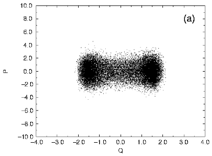
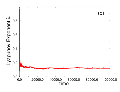
FIG. 1.: Quantum chaotic attractor for one realization with parameters: $\hbar\equiv 1$, $a=10$, $b=4$, $\gamma=0.002$. (a) The Poincaré section $Q$-$P$ taken by $\alpha=0\pm 0.0015$ and $\dot{\alpha}\geq 0$; (b) The time evolution of the largest Lyapunov exponent $\lambda$. For this realization, the sum of all Lyapunov exponents in phase space $\sum_{i}\lambda_{i}\simeq-4.011\times 10^{-3}$ and the fractal dimension $D_{f}\simeq 3.968$.

FIG. 2.: The simulation for $1000$ realizations with the same parameters as in Fig. 1. (a) The distribution $D(\lambda)$ of the largest Lyapunov exponents with $\int d\lambda D(\lambda)=1$. The mean $\lambda_{\rm largest}\simeq 0.127$, $D_{f}\simeq 3.969$ and $\sum_{i}\lambda_{i}\simeq-3.957\times 10^{-3}$. Lyapunov exponents are calculated by means of Wolf et al [21]. (b) The probability map, taking constant $Q=1.581\pm 0.05$ (near the bottom of one potential well) and $\tau=5$. This map starts after a relaxation time of $10000$.

REFERENCES

- [1] Chaos and quantum physics: 1989 Les Houches Summer School, ed. by M. -J. Giannoni, A. Voros, and J. Zinn-Justin, (North-Holland, Amsterdam, 1991).
- [2] L. E. Reichl, The Transition to Chaos in Conservative Systems: Quantum Manifestations (Springer-Verlag, New York, 1992).
- [3] A. K. Pattanayak and W. C. Schieve, Phys. Rev. Lett. 72, 2855 (1994).
- [4] Y. Ashkenazy, L. P. Horwitz, J. Levitan, M. Lewkowicz, and Y. Rothschild, Phys. Rev. Lett. 75, 1070 (1995).
- [5] T. P. Spiller and J. F. Ralph, Phys. Lett. A 194, 235 (1994) and reference therein.
- [6] G. Lindblad, Commun. Math. Phys. 48, 119 (1976).
- [7] R. Schack, T. A. Brun, and I. C. Percival, J. Phys. A: Math. Gen. 28, 5401 (1995).
- [8] T. A. Brun, Phys. lett. A 206, 167 (1995).
- [9] R. P. Feynman and F. L. Vernon Jr., Ann. Phys. (N.Y.) 24, 118 (1963).
- [10] A. O. Caldeira and A. J. Leggett, Physica 121A, 587 (1983).
- [11] C. W. Gardiner, Quantum Noise (Springer, Berlin, 1991), Chap. 3.
- [12] Other procedures to deal with dissipation can be found in, for example, G. Parisi, Statistical Field Theory (Addison-Wesley, Redwood, 1988), Ch. 18, and reference therein, for the stochastic formulation of quantum mechanics.
- [13] This technique with its applications was discussed in Sects. 3.5, 3.7 and 9.3 of Ref. [11].
- [14] This was given in Ref. [11]. Since the high frequency behavior of the spectral function is proportional to and so is very badly behaved in noise theory, we have to impose a high frequency cutoff by introducing . The physical justification for this comes from the form (2), where the factor comes into play. This factor must drop off sufficiently rapidly at high frequencies because for wavelengths shorter than a wave of displacements of atoms becomes meaningless.
- [15] A. M. Perelmov, Generalized Coherent States and their Applications (Springer-Verlag, Berlin, 1986) and reference therein.
- [16] R. Jackiw and A. Kerman, Phys. Lett. A 71, 158 (1979).
- [17] E. J. Heller, in Ref. [1]; see also, E. J. Heller and S. Tomsovic, Phys. Today 46 (7), 38 (1993).
- [18] Y. Tsue, Prog. Theor. Phys. 88, 911 (1992).
- [19] For details, see, W. V. Liu and W. C. Schieve, (in preparation).
- [20] A. K. Pattanayak and W. C. Schieve, Phys. Rev. E 50, 3601 (1994).
- [21] A. Wolf, J. B. Swift, H. L. Swinney, and J. A. Vastano, Physica 16D, 285 (1985).
- [22] H. G. Schuster, Deterministic Chaos (VCH, Weinheim, 1995), sec. 5.2.
- [23] T. Kapitaniak, Chaos in System with Noise (World Scientific, Singapore, 1988).
- [24] Because we have only run realizations (so the accuracy of cannot be better than ), the map seems to contain only finite elements. We argue that for an infinite number of realizations (i.e., in the thermodynamical limit) the map shall consist of infinite number of points.
- [25] W. C. Schieve and A. R. Bulsara, Phys. Rev. A 41, 1172 (1990); A. R. Bulsara, E. W. Jacobs, and W. C. Schieve, Phys. Rev. A 42, 4614 (1990).