Boundary contributions to the semiclassical traces
of the baker’s map

¹Centro Brasileiro de Pesquisas Físicas

Rua Xavier Sigaud 150, CEP 22290-180, RJ, Rio de Janeiro, Brazil

²Service de Physique Théorique,

Commissariat à l’Energie Atomique–Centre d’Etudes Nucléaires de Saclay,

F–91191 Gif–sur–Yvette CEDEX, France

³Centre Emile Borel, Institut Henri Poincaré,

11 Rue Pierre et Marie Curie, 75231 Paris Cedex, France

Abstract

We evaluate the leading asymptotic contributions to the traces of the quantum baker’s map propagator. Besides the usual Gutzwiller periodic orbit contribution, we identify boundary paths giving rise to anomalous $\log\hbar$ terms. Some examples of these anomalous terms are calculated both numerically and analytically.

1 Introduction

The usual derivation of the periodic orbit trace formula for chaotic systems extracts as stationary phases the actions of isolated periodic orbits while the amplitudes are given by the contributions of their hyperbolic neighbourhoods. However, when the orbits lie on discontinuities or at the boundary of classically allowed regions, anomalous contributions are expected.[1] We analize and calculate the origin of these contributions for the simplest piecewise–linear map: the baker’s transformation.

In spite of many generic properties and its inherent simplicity, the baker’s map has shown some ”anomalies”, both in the statistical properties of the quasi–energy spectrum[2] and in the asymptotic behaviour of the lowest traces of the propagator.[3] It is now understood that these anomalies are related to the discontinuous way in which the map transforms phase space and to the singular nature of the fixed point:[4] it lies on the discontinuity and does not have a whole hyperbolic vicinity (in this sense, all the other periodic points are regular). In Ref. [3] it was shown that, when the map is quantized, and its semiclassical traces considered in the context of periodic orbit theory, the contributions coming from singular symbols (related to the fixed point and its repetitions) show anomalous terms with a $\log\hbar$ dependence. Some indications of anomalous behaviour for regular symbols (related to regular periodic orbits) were also communicated.

Our main result is that not only the singular symbols contribute anomalously to the trace but every regular symbol also does. We trace these contributions to classical paths (not periodic orbits) whose action is stationary at the vertices of classically allowed (hypercube–shaped) domains.

The paper is organized as follows. In Section 2 we briefly review the classical and quantum features of the map that will be relevant for further discussions. Section 3 describes the manipulations on the iterated propagator that lead to an exact symbolic decomposition of its traces. The exact contribution to the trace from each symbol sequence results in a path summation formula which, following a procedure suggested in Ref. [5], is converted by Poisson transformation into a multiple infinite number of (continuous variables) path integrals in phase space. This is the starting point for the approximations to be made.

In Section 4 we analize the different stationary paths that contribute to these integrals and their charachteristic $\hbar$ dependence, thus obtaining their asymptotic behaviour. We arrive at the result that, for each symbol, the asymptotic behaviour is ruled by more than one path. The periodic orbit (labeled with that symbol) contributes with the usual Gutzwiller term and a vertex path contributes with a logarithmic term. Some examples of these anomalous terms are calculated, both analytically and numerically. Further constant terms arising from other stationary paths are identified but are very hard to calculate. Section 5 contains the concluding remarks.

2 Review of the classical and quantum baker’s map

In this section we display the well known classical and quantum ingredients of the baker’s that will be needed for further analysis.

The classical baker’s transformation is an area preserving, piecewise–linear map of the unit square (periodic boundary conditions are assumed) defined as

$$p_{1}=\frac{1}{2}(p_{0}+\epsilon_{0})~{},~{}~{}~{}q_{1}=2q_{0}-\epsilon_{0}~{};$$ (1)

where $\epsilon_{0}=[2q_{0}]$, the integer part of $2q_{0}$. This map is known to be uniformly hyperbolic, the stability exponent for orbits of period $L$ being $L\log 2$. Moreover it admits a useful description in terms of a complete symbolic dynamics. A one to one correspondence between phase space coordinates and binary sequences,

$$(p,q)\leftrightarrow\ldots\epsilon_{-2}\epsilon_{-1}\cdot\epsilon_{0}\epsilon_{1}\epsilon_{2}\ldots~{}~{}~{},~{}\epsilon_{i}=0,1~{},$$ (2)

can be constructed in such a way that the action of the map is conjugated to a shift map. The symbols are assigned as follows: $\epsilon_{i}$ is set to zero (one) when the $i$–th iteration of $(p,q)$ falls to the left (right) of the line $q=1/2$, i.e. $[2q_{i}]=\epsilon_{i}$. Reciprocally, given an itinerary $\ldots\epsilon_{-2}\epsilon_{-1}\cdot\epsilon_{0}\epsilon_{1}\epsilon_{2}\ldots$, the related phase point is obtained through the especially simple binary expansions

$$q=\sum_{i=0}^{\infty}\frac{\epsilon_{i}}{2^{i+1}}~{},~{}~{}~{}p=\sum_{i=1}^{\infty}\frac{\epsilon_{-i}}{2^{i}}~{}.$$ (3)

Once the dynamics has been mapped to a shift on binary sequences it is very easy to analize the dynamical features of the map. In particular, periodic points are associated to infinite repetitions of finite sequences of symbols. It will be convenient for later purposes to introduce a vector notation for these sequences so that $\mbox{\boldmath$\epsilon$}=(\epsilon_{0},\epsilon_{1},\ldots,\epsilon_{L-1})^{t}$ (the superscript means transposition). We also denote the positions and momenta of a periodic trajectory of length $L$ as ${\bf q}^{*}$=$(q^{*}_{0},q^{*}_{1},\ldots,q^{*}_{L-1})^{t}$ and ${\bf p}^{*}$=$(p^{*}_{0},p^{*}_{1},\ldots,p^{*}_{L-1})^{t}$. For a given $\epsilon$, the initial point on the trajectory is obtained by considering a periodic itinerary of length $L$ in (3)[6]

$$q_{0}^{*}=\frac{1}{2^{L}-1}\sum_{i=0}^{L-1}{2^{L-1-i}\,\epsilon_{i}}~{},~{}~{}~{}p_{0}^{*}=\frac{1}{2^{L}-1}\sum_{i=0}^{L-1}{2^{i}\,\epsilon_{i}}~{}.$$ (4)

The other points are obtained by shifting cyclically the binaries $\epsilon_{i}$ in the expression above. In a compact form,

$${\bf q}^{*}={\bf A}^{-1}\,\mbox{\boldmath$\epsilon$}~{},~{}~{}~{}{\bf p}^{*}=({\bf A}^{t})^{-1}\,{\bf S}\,\mbox{\boldmath$\epsilon$}~{}.$$ (5)

The matrix ${\bf A}^{-1}$ is directly related to the matrix ${\bf S}$ of a cyclic shift, ${\bf S}\cdot(a_{0},a_{1},\ldots a_{L-1})^{t}=(a_{1},\ldots,a_{L-1},a_{0})^{t}$,

$${\bf A}^{-1}=\frac{1}{2^{L}-1}\sum_{i=0}^{L-1}{2^{L-1-i}\,{\bf S}^{i}}~{},$$ (6)

and embodies all the symmetries of the periodic trajectories.[6] Its inverse will play an important role in the quantum and semiclassical analysis and has the simple form,

$${\bf A}={\bf 2}-{\bf S}~{}.$$ (7)

Due to its piecewise linear nature, the baker’s map admits a (mixed) generating function which is a piecewise bilinear form,

$$W_{\epsilon_{0}}(p_{1},q_{0})=2p_{1}q_{0}-\epsilon_{0}p_{1}-\epsilon_{0}q_{0}~{},~{}~{}~{}\epsilon_{0}=0,1~{}.$$ (8)

It is not defined on the whole space $p_{1}$–$q_{0}$ but on the classically allowed domains

$$R_{0}=[0,1/2]\times[0,1/2]~{}~{}~{}\mbox{and}~{}~{}~{}R_{1}=[1/2,1]\times[1/2,1]~{}.$$ (9)

Once the generating function is defined, actions can be assigned to the periodic orbits.[7] In our notation they read

$$S_{\mbox{\scriptsize\boldmath$\epsilon$}}=\mbox{\boldmath$\epsilon$}^{t}\,{\bf A}^{-1}\,\mbox{\boldmath$\epsilon$}=({\bf S}{\bf p}^{*})^{t}\,{\bf A}\,{\bf q}^{*}~{}.$$ (10)

With respect to the quantum map, we will follow the original quantization of Balazs and Voros[8], as later modified in Ref. [6] to preserve in the quantum map all the symmetries of its classical counterpart. In the mixed representation the baker’s propagator can be written as an $N\times N$ block–matrix ($N$ even):

$$\langle p_{m}|B_{N}|q_{n}\rangle=\left(\begin{array}[]{cc}G_{N/2}&0\\ 0&G_{N/2}\end{array}\right)~{},$$ (11)

where position and momentum eigenvalues run on a discrete mesh with step $1/N=h$ ($h$ = Planck’s constant), so that

$$q_{n}=(n+1/2)/N~{},~{}~{}~{}p_{m}=(m+1/2)/N~{},~{}~{}~{}0\leq n,m\leq N-1~{};$$ (12)

and $G_{N}$ is the antiperiodic Fourier matrix, which transforms from the $q$ to the $p$ basis,

$$G_{N}=\langle p_{m}|q_{n}\rangle=(1/\sqrt{N})e^{-2\pi iNp_{m}q_{n}}~{}.$$ (13)

This propagator[7] has the standard structure of quantized linear symplectic maps,

$$\langle p_{m}|B|q_{n}\rangle=\left\{\begin{array}[]{cl}\sqrt{2/N}\,e^{-i2\pi NW_{0}(p_{m},q_{n})}&\mbox{if}~{}~{}(p_{m},q_{n})\,\in\,R_{0}\\ \sqrt{2/N}\,e^{-i2\pi NW_{1}(p_{m},q_{n})}&\mbox{if}~{}~{}(p_{m},q_{n})\,\in\,R_{1}\\ 0&\mbox{otherwise}~{}.\end{array}\right.$$ (14)

In this quantization, only those transitions are allowed that respect the rule $[2p_{m}]=[2q_{n}]$, a reflection of the classical shift property.

3 Path integral formulation

The iteration of the propagator in the mixed representation is simply the expansion of a finite matrix product, which we write as

$$\langle p_{L}|B^{L}|q_{0}\rangle=\sum\langle p_{L}|B|q_{L-1}\rangle\langle q_{L-1}|p_{L-1}\rangle\cdots\langle p_{2}|B|q_{1}\rangle\langle q_{1}|p_{1}\rangle\langle p_{1}|B|q_{0}\rangle~{},$$ (15)

where the summation is over repeated phase space coordinates. To simplify notation we have dropped the subindices labeling the discrete values of the coordinates in (12) in favor of a subindex labeling the (discrete) time on the trajectory. When (14) is taken into account the trace of the iterated propagator can be written as a sum over paths of length $L$

$$\mbox{Tr}B^{L}=\sum_{\gamma}A_{\gamma}\,e^{iW_{\gamma}/\hbar}~{},$$ (16)

where $A_{\gamma}$ is the amplitude and $W_{\gamma}$ the action of a path $\gamma=(q_{0},p_{1},q_{1},p_{2},\cdots,q_{L-1},p_{L})$ which satisfies the rule $[2q_{i}]=[2p_{i+1}]$. By grouping the paths according to their symbolic itinerary $\mbox{\boldmath$\epsilon$}=(\epsilon_{0},\epsilon_{1},\ldots,\epsilon_{L-1})$, the trace can be further decomposed as $\mbox{Tr}B^{L}=\sum_{\mbox{\scriptsize\boldmath$\epsilon$}}\mbox{Tr}B_{\mbox{\scriptsize\boldmath$\epsilon$}}^{L}$, with

$$\mbox{Tr}B_{\mbox{\scriptsize\boldmath$\epsilon$}}^{L}=\frac{2^{L/2}}{N^{L}}\sum e^{-2\pi iN\,[W_{\epsilon_{0}}(q_{0},p_{1})-q_{1}p_{1}+W_{\epsilon_{1}}(q_{1},p_{2})-\cdots-q_{L-1}p_{L-1}+W_{\epsilon_{L-1}}(q_{L-1},p_{L})-q_{0}p_{L}]}~{}.$$ (17)

This decomposition breaks up the trace of the propagator into partial sums each one labeled by a symbolic code. Contrary to the usual semiclassical procedure, this decomposition is now exact. Each symbol, instead of corresponding semiclassically to a Gutzwiller contribution from a periodic orbit is given by a sum over paths that share a common symbolic code. The asymptotic evaluation of these sums can now be attempted focusing on one symbol at a time. Thus from now on we restrict the analysis to the partial trace $\mbox{Tr}B_{\mbox{\scriptsize\boldmath$\epsilon$}}^{L}$, i.e. we take $\epsilon$ fixed.

As a function of continuous coordinates, the quadratic phase in (17) has the property of being stationary over the only periodic trajectory carrying the label $\epsilon$ (for $N$ big enough, a discrete path arbitrarily close to this trajectory can be found, so the stationary phase picture also holds in the discrete case). A first attempt at the semiclassical evaluation of (17)[7] consisted in replacing the sums by integrals which can then be evaluated in the stationary phase approximation, neglecting boundary contributions. (Special care has to be taken of the anomalous contributions of the fixed point and its repetitions: these trajectories lie on a vertex of the domain of integration, where the approximations stated before are not applicable.) In the case of regular orbits, i.e. $\mbox{\boldmath$\epsilon$}\neq(0,0,\cdots,0)$ and $\mbox{\boldmath$\epsilon$}\neq(1,1,\cdots,1)$, this procedure leads to the usual semiclassical expression

$$\mbox{Tr}B_{\mbox{\scriptsize\boldmath$\epsilon$}}^{L}\approx\frac{2^{L/2}}{2^{L}-1}\,e^{2\pi iNS_{\mbox{\scriptsize\boldmath$\epsilon$}}}~{},$$ (18)

where $S_{\mbox{\scriptsize\boldmath$\epsilon$}}$ is the action of the (stationary phase) periodic orbit given in (10). This result, combined with an ad hoc evaluation of the anomalous fixed points contributions led to a fairly good reconstruction of the smoothed properties of the spectrum.[7] However, a more careful semiclassical analysis of the first traces[3] revealed the existence of anomalous contributions, typically terms of the order $\log\hbar$. The presence of these terms was then interpreted as coming from the singular orbits; nevertheless, certain quantitative differences could not be explained, moreover, anomalous behaviour of a regular orbit was also suggested.[3]

In this paper we explain the reason for the failure of previous attempts to obtain asymptotic expressions for the traces which is intimately linked to the discreteness of the coordinate grid. Another path–not a trajectory–exists that renders the phase stationary. Small discrete displacements about this path produce a (leading order) variation of the phase which is an integer multiple of $2\pi$. This is a path of quasi–stationary phase, related to aliasing; it lies at a vertex of the space of paths, and thus escapes the usual stationary phase treatment. This phenomenon occurs for all symbols and therefore all traces are anomalous in this sense. The correct trace expansion for each symbol should then be written as

$$\mbox{Tr}B_{\mbox{\scriptsize\boldmath$\epsilon$}}^{L}\approx\frac{2^{L/2}}{2^{L}-1}\,e^{2\pi iNS_{\mbox{\scriptsize\boldmath$\epsilon$}}}+a_{\mbox{\scriptsize\boldmath$\epsilon$}}\log N+b_{\mbox{\scriptsize\boldmath$\epsilon$}}+\ldots~{},$$ (19)

where the first term will be absent for $\mbox{\boldmath$\epsilon$}={\bf 0}$ or ${\bf 1}$ ($a_{\mbox{\scriptsize\boldmath$\epsilon$}}$ and $b_{\mbox{\scriptsize\boldmath$\epsilon$}}$ are complex constants).

In order to clearly display the abovementioned features we follow Ref. [5] and transform the path summation into integrations via the Poisson formula. Making use of the identity

$$\sum_{i=0\,(\frac{N}{2})}^{\frac{N}{2}-1\,(N-1)}F(q_{i})=N\sum_{K=-\infty}^{\infty}(-1)^{K}\int_{0\,(\frac{1}{2})}^{\frac{1}{2}\,(1)}\,e^{2\pi iNKq}\,F(q)\,dq~{},$$ (20)

where the parenthesis indicate alternative ranges for the summation (integration), we rewrite (17) as

$$\mbox{Tr}B_{\mbox{\scriptsize\boldmath$\epsilon$}}^{L} = 2^{L/2}N^{L}\sum_{M_{0}}\cdots\sum_{M_{L-1}}\sum_{K_{1}}\cdots\sum_{K_{L}}(-)^{M_{0}+\ldots+M_{L-1}+K_{1}+\ldots+K_{L}}\times$$ (21)

$$\times \int_{R_{\epsilon_{0}}}dq_{0}dp_{1}\int_{R_{\epsilon_{1}}}dq_{1}dp_{2}\cdots\int_{R_{\epsilon_{L-1}}}dq_{L-1}dp_{L}\,e^{-2\pi iN\phi}~{}.$$

$M_{i},K_{i}$ come from Poisson transforming the variables $q_{i},p_{i}$ and take all integer values. The phase $\phi$ is

$$\phi = W_{\epsilon_{0}}(q_{0},p_{1})-p_{1}q_{1}-M_{0}q_{0}-K_{1}p_{1}+W_{\epsilon_{1}}(q_{1},p_{2})-p_{2}q_{2}-M_{1}q_{1}-K_{2}p_{2}+\cdots$$ (22)

$$\cdots+W_{\epsilon_{L-1}}(q_{L-1},p_{L})-p_{L}q_{0}-M_{L-1}q_{L-1}-K_{L}p_{L}~{}.$$

In a more compact form we write

$$\mbox{Tr}B_{\mbox{\scriptsize\boldmath$\epsilon$}}^{L}=\sum_{M,K}(-)^{M_{0}+\ldots+M_{L-1}+K_{1}+\ldots+K_{L}}I_{\epsilon,M,K}~{},$$ (23)

implicitly defining the integrals $I_{\epsilon,M,K}$.

This is the starting point of the semiclassical analysis (cf. (17)). Standard stationary phase is now possible as sums have been replaced by integrals–in an exact way. The difficulty now is that we have to deal with an infinite multiplicity of integrals and therefore it is essential for further progress to identify among them those that contribute significantly to the asymptotic behaviour. At this point our treatment diverges from that in Ref. [5] where a truncation of the Poisson expansion was considered. On one side, the truncation misses constant terms which come from infinite families of integrals (Appendix A). On the other, the truncated set contains integrals which are not relevant in the far asymptotic regime, as only a few specific ones are needed (next section).

4 The semiclassical trace formula

In analizing the traces as given by (23) we follow the criterion that the most important contributions will come from those multiple integrals having stationary phase paths lying in the interior of the domains of integration (or on the boundary). Other cases will be oscillatory over the whole domain and thus contribute vanishingly.

For compactness we will use the matrix notation introduced earlier. The positions and momenta of a path of length $L$ will be respectively denoted ${\bf q}$=$(q_{0},q_{1},\ldots,q_{L-1})^{t}$ and ${\bf p}$=$(p_{1},\ldots,p_{L})^{t}$. Analogously we define the vectors of integers coming from the Poisson transformation: ${\bf M}$=$(M_{0},\ldots,M_{L-1})^{t}$ and ${\bf K}$=$(K_{1},\ldots,K_{L})^{t}$. For convenience of notation notice that here ${\bf p}$ is shifted with respect to that defined in Section 2. All vectors and matrices will be understood to be $L$–dimensional.

The quadratic character of the generating function (8) can be used to express the phase $\phi$ (22) of a path contributing to the partial trace $\mbox{Tr}B_{\mbox{\scriptsize\boldmath$\epsilon$}}^{L}$, and corresponding to Poisson integers ${\bf M}$ and ${\bf K}$, as

$$\phi={\bf p}^{t}\,{\bf A}\,{\bf q}-{\bf p}^{t}\,(\mbox{\boldmath$\epsilon$}+{\bf K})-{\bf q}^{t}\,(\mbox{\boldmath$\epsilon$}+{\bf M})~{};$$ (24)

${\bf A}$ and its inverse were defined in (6, 7). A stationary phase path $(\tilde{\bf q},\tilde{\bf p})$ is then a solution of the equations $\nabla_{\bf q}\,\phi=0$, $\nabla_{\bf p}\,\phi=0$, that is,

$$\tilde{\bf q}={\bf A}^{-1}\,(\mbox{\boldmath$\epsilon$}+{\bf K})~{},~{}~{}~{}\tilde{\bf p}=({\bf A}^{t})^{-1}\,(\mbox{\boldmath$\epsilon$}+{\bf M})~{}.$$ (25)

Equivalently, these stationary points could have been identified in the discrete picture (17) by requiring the quasistationarity of the action $W$, i.e. $\nabla_{\bf q}\,W={\bf M}$, $\nabla_{\bf p}\,W={\bf K}$. The advantage of having introduced the Poisson’s transformation is that it is now clear how to calculate the contribution of each stationary path. For fixed $\epsilon$, (25) gives one solution for each choice of K and M. The quadratic form, shifted to this stationary point becomes

$$\phi=({\bf p}-\tilde{\bf p})^{t}\,{\bf A}\,({\bf q}-\tilde{\bf q})-\tilde{\bf p}^{t}\,{\bf A}\,\tilde{\bf q}~{}.$$ (26)

The point $(\tilde{\bf q},\tilde{\bf p})$ may fall inside, on the vertices or faces, or outside the region of integration $R_{\epsilon_{0}}\times R_{\epsilon_{1}}\times\ldots\times R_{\epsilon_{L-1}}$. There are only three kinds of solutions (25) that do not fall outside the domain of integration:

• Interior paths. These paths coincide with the regular periodic trajectories (5) and are obtained by setting K and M to zero for $\mbox{\boldmath$\epsilon$}\neq\bf{0},\bf{1}$. The corresponding coordinates are $\tilde{\bf q}={\bf q}^{*}$ and $\tilde{\bf p}={\bf S}\,{\bf p}^{*}$. The stationary value of the phase, $\tilde{\phi}\/$, is the classical action of the trajectory, i.e. $\tilde{\phi}=S_{\mbox{\scriptsize\boldmath$\epsilon$}}\/$ (see Section 2).

• Vertex paths. By choosing ${\bf K}=({\bf A}-1)\mbox{\boldmath$\epsilon$}$ and ${\bf M}=({\bf A}^{t}-1)\mbox{\boldmath$\epsilon$}$, we get the solution $\tilde{\bf q}=\mbox{\boldmath$\epsilon$}$, $\tilde{\bf p}=\mbox{\boldmath$\epsilon$}$. The corresponding value for the phase, $\tilde{\phi}=\mbox{\boldmath$\epsilon$}^{t}\,{\bf A}\,\mbox{\boldmath$\epsilon$}$, is an integer, and so has no relevance in the phase in (21).

• There are two face paths. Their coordinates are obtained by mixing regular and vertex solutions, i.e. $(\tilde{\bf p},\tilde{\bf q})$=$(\mbox{\boldmath$\epsilon$},{\bf q}^{*})$ or $({\bf p}^{*},\mbox{\boldmath$\epsilon$})$.

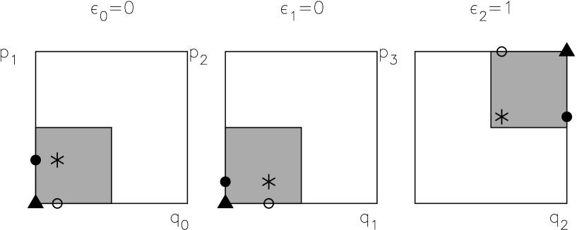
Figure 1: Stationary phase paths associated to the regular symbol $\mbox{\boldmath$\epsilon$}=(0,0,1)$. The space of allowed paths is a hypercube of side 1/2 (gray squares). The interior path ($\ast$) corresponds to a periodic trajectory and gives rise to the usual Gutzwiller term in the trace formula. The vertex path ($\triangle$) and its anomalous vicinity are responsible for the $\log\hbar$ term. ”Face” paths ($\circ$, $\bullet$) contribute with constant terms.

It must be pointed out that in the case of the singular symbols $\mbox{\boldmath$\epsilon$}=\bf{0},\bf{1}$ there is only one solution–the vertex one. In Fig. 1 we show as an example the stationary paths for the case $L=3$ and the regular symbol $\mbox{\boldmath$\epsilon$}=(0,0,1)$.

In the first case (R), the asymptotic evaluation of the integral is straightforward. The stationary path coincides with a regular periodic orbit and it is interior to the integration domain, therefore boundary terms can be neglected. The quadratic form can be brought to principal axes and evaluated in a standard way. The result is simply

$$\mbox{I}_{\mbox{\scriptsize\boldmath$\epsilon$}}^{R} = 2^{L/2}\,e^{2\pi iNS_{\mbox{\scriptsize\boldmath$\epsilon$}}}N^{L}\times\int_{R_{\mbox{\scriptsize\boldmath$\epsilon$}}}\,d{\bf p}\,d{\bf q}\,e^{-2\pi iN\,({\bf p}-\tilde{\bf p})^{t}\,{\bf A}\,({\bf q}-\tilde{\bf q})}=$$ (27)

$$= \frac{2^{L/2}}{2^{L}-1}\,e^{2\pi iNS_{\mbox{\scriptsize\boldmath$\epsilon$}}}+\mbox{terms decreasing with $N$}~{},$$

the usual Gutzwiller contribution (we have used $\det{\bf A}=2^{L}-1$).

For vertex (V) solutions this procedure is not possible because the neighbourhood of the path (which only coincides with a periodic trajectory when $\mbox{\boldmath$\epsilon$}=\bf{0},\bf{1}$) is intersected by the boundaries of the hypercube of integration. The integral to be evaluated can be brought to the form (using the new coordinates ${\bf q}-\mbox{\boldmath$\epsilon$}$ and ${\bf p}-\mbox{\boldmath$\epsilon$}$)

$$\mbox{I}_{\mbox{\scriptsize\boldmath$\epsilon$}}^{V}=2^{L/2}N^{L}\times\int_{[0,\frac{1}{2}]^{2L}}\,d{\bf p}\,d{\bf q}\,e^{-2\pi iN\,{\bf p}^{t}\,{\bf J}_{\mbox{\scriptsize\boldmath$\epsilon$}}\,{\bf A}\,{\bf J}_{\mbox{\scriptsize\boldmath$\epsilon$}}\,{\bf q}}~{}.$$ (28)

${\bf J}_{\mbox{\scriptsize\boldmath$\epsilon$}}$ is a diagonal matrix with elements $\pm 1$, $J_{ii}=1-2\epsilon_{i-1}~{},~{}1\leq i\leq L~{},$ and contains the dependence on the symbol $\epsilon$.

(A comment about the invariant properties of (28) is in order. The original path sum (17) is cyclically invariant with respect to shifts on the symbol $\epsilon$ and also respects all the symmetries of the map.[3] Once the stationary paths have been identified and their contributions evaluated it is important to verify that these symmetries are maintained. In that case, only one representative integral for each symbol and symmetry class needs calculation. From the expression (28) it is possible to check that this is indeed the case.)

To our knowledge, for $L>2$, the leading asymptotic expression for the integral (28) cannot be evaluated analytically. Appendix B presents the case $\mbox{I}_{(0,1)}^{V}$ as an example of the difficulties involved in such calculations. The analytical and numerical results for the shortest symbols indicate that $\mbox{I}_{\mbox{\scriptsize\boldmath$\epsilon$}}^{V}$ displays the following asymptotic behavior ($N\!\rightarrow\!\infty$),

$$I_{\mbox{\scriptsize\boldmath$\epsilon$}}^{V}=a_{\mbox{\scriptsize\boldmath$\epsilon$}}\ln N+b_{\mbox{\scriptsize\boldmath$\epsilon$}}+\mbox{decreasing terms}~{},$$ (29)

where $a_{\mbox{\scriptsize\boldmath$\epsilon$}}$ and $b_{\mbox{\scriptsize\boldmath$\epsilon$}}$ are (complex) constants. For $L=1,2$ this result is obtained analytically, for $L=3$, numerically.

The simplest example of a vertex integral is that associated to the calculation of the first trace, worked out in the Appendix A. In this case the only stationary path is the vertex one, there are no interior nor face paths. It is shown that asymptotically the vertex integrals $I_{\mbox{\scriptsize\boldmath$\epsilon$}=(0)}^{V}$ and $I_{\mbox{\scriptsize\boldmath$\epsilon$}=(1)}^{V}$ give account of the $\log N$ term, but fail in reproducing the constant one which is present in $\mbox{Tr}B_{\mbox{\scriptsize\boldmath$\epsilon$}=(0)}$. It is also proven that to obtain the correct constant an additional infinite family of Poisson integrals must be considered. These integrals, which provide a constant term, contain continuous sets of stationary points of the second kind,[9] i.e. their phases are stationary with respect to displacements along the faces of the hypercube of integration. We expect that in the general case ($L>1$) this behaviour will be maintained: the vertex integral will provide the correct $\log N$ term, but the constant $b_{\mbox{\scriptsize\boldmath$\epsilon$}}$ will only be obtained when an infinite family of Poisson integrals is calculated. So, even though constant terms in the trace expansion are detected, its calculation is very hard and will not be attempted here.

As to face solutions (F), there is numerical evidence that these integrals will contribute with a constant.[10] On the basis of the previous discussion, we subordinate their study to further progress in the identification and handling of the infinite families of integrals of the second kind that are also responsible for the constant term.

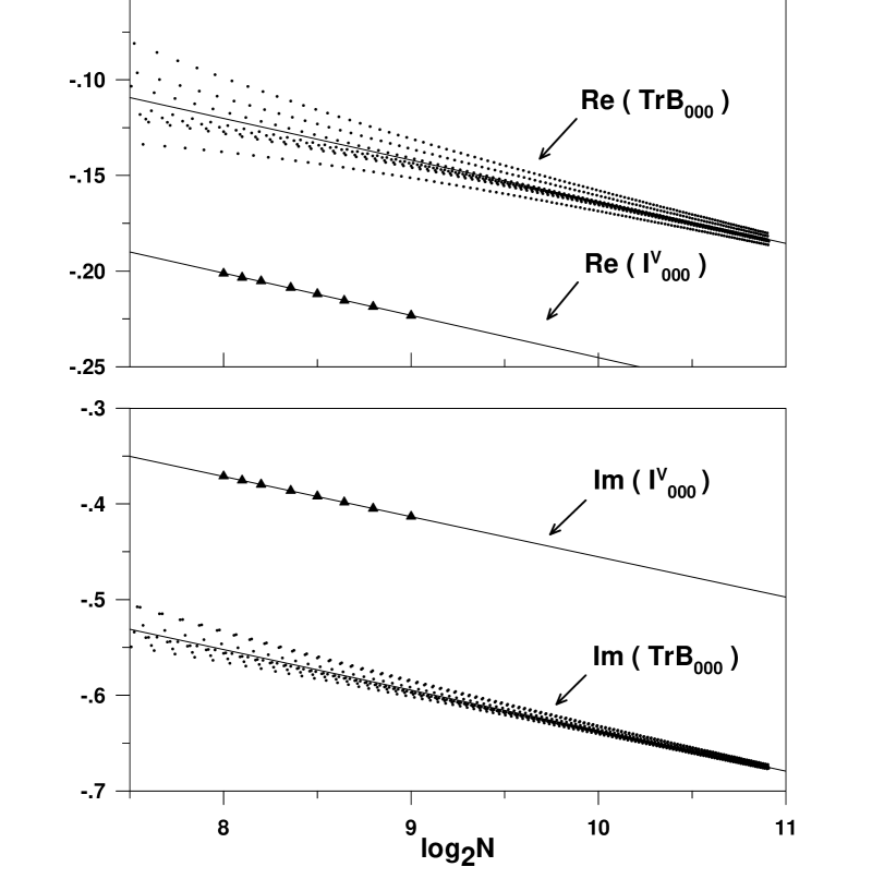
Figure 3: The exact trace $\mbox{Tr}B_{(0,0,0)}$ as a function of $\log_{2}N$ together with the corresponding vertex integral $I_{(0,0,0)}^{V}$.

In Figs. 2 and 3 we show, for the case $L=3$, numerical data concerning the asymptotic behaviour of the exact traces as calculated by matrix multiplication (17) and the prediction of our theory, i.e. the associated vertex integrals (29). The representative traces $\mbox{Tr}B_{(0,0,0)}$ and $\mbox{Tr}B_{(0,0,1)}$ are plotted as a function of even $N$ (in the second case the Gutzwiller term has been substracted) together with some values of the vertex integrals $I_{(0,0,0)}^{V}$ and $I_{(0,0,1)}^{V}$ (much more time demanding than the traces). The straight lines are obtained by means of linear fits to the numerical data (in the case of the traces only a subsequence of points with $N>2^{10}$ has been taken into account). These figures show clearly that the vertex integral captures the correct $\log N$ dependence but that the constant is incorrect. This is exactly the same behaviour that is calculated analytically for the cases $L=1,2$. The high quality of this agreement can be observed in Table 1, where a quantitative comparison between the asymptotics of traces and integrals is displayed. There we exhibit the coefficients $a_{\mbox{\scriptsize\boldmath$\epsilon$}}$ of the $\log N$ terms as extracted either from linear fits or analytically (Appendices A and B, Ref. [3]). A representative member of each symmetry class up to $L=3$ is shown.

Notice that the $\log N$ dependence does not dissappear in the full traces and therefore it is not an artifice of the symbolic decomposition. For instance for $L=3$ we have $\mbox{Tr}B^{3}=2\mbox{Tr}B_{(0,0,0)}+6\mbox{Tr}B_{(0,0,1)}$ and from Table 1 we get $\mbox{Tr}B^{3}\approx(-0.126-i\,0.103)\log N$.

5 Concluding remarks

We have shown that stationary phase paths other than periodic trajectories exist which significantly contribute to the semiclassical trace formula of the quantum baker’s map. The fact that these paths lie on vertices or faces of the allowed phase space makes their contribution anomalous: they give rise to $\log\hbar$ and other terms. A theory is presented that not only explains the origin of those anomalies but is capable of quantitative predictions. In the case of the three shortest traces, these predictions are compared to the exact results showing excellent agreement. These results encourage us to conjecture that all partial traces will display this behaviour. So, the semiclassical trace formula for the baker’s map becomes

$$\mbox{Tr}B^{L}=\sum_{\mbox{\scriptsize\boldmath$\epsilon$}}{(a_{\mbox{\scriptsize\boldmath$\epsilon$}}\log N+b_{\mbox{\scriptsize\boldmath$\epsilon$}})}+\sum_{\mbox{\scriptsize\boldmath$\epsilon$}\neq{\bf 0,1}}{\frac{2^{L/2}}{2^{L}-1}\,e^{2\pi iNS_{\mbox{\scriptsize\boldmath$\epsilon$}}}}+\mbox{decreasing terms}~{}.$$ (30)

Each coefficient $a_{\mbox{\scriptsize\boldmath$\epsilon$}}$ involves the calculation of a multidimensional integral, which, up to now, must be done numerically. These integrals adopt the simple form of a quadratic phase which is stationary on the vertex of an hypercube. This seems to be a complicated task but maybe not unsolvable. The calculation of the constant terms $b_{\mbox{\scriptsize\boldmath$\epsilon$}}$ in the expansion is even a more difficult problem, as it involves the identification and handling of infinite families of integrals (dominated by second kind stationary points).

Even though the results presented here have been obtained for a particular quantization of the baker’s map, we believe that these results are extendible to any quantization (e.g. the optical baker[11]), as they are a consequence of the unusual nature of the fixed point of the classical map, which lies on a discontinuity. However, the particular values of the coefficients in the trace formula may depend of the particular scheme used to quantize the map.

The trace formula –without the $\log N$ terms– was tested numerically both for smoothed spectral properties using the density of states[7] and for individual eigenvalues using zeta-function techniques.[3] In both cases, for computational reasons, $N$ was restricted to take relatively small values (e.g. $N=48$ in [3], $N$ up to 1024 in [7]). The agreement obtained was remarkable and can be explained by the fact that for such low values the $\log N$ terms do not play a significant role. It remains the open question, in view of our present results, if that agreement is truly asymptotic or if it will deteriorate for larger values of $N$.

Appendix A

In this appendix we study the asymptotics of the first trace of the map. The result has been obtained in Ref. [3] with an ad hoc procedure to evaluate the sums. Here we show how to arrive at the same result but using stationary phase considerations in the context of the Poisson expansion. This example illustrates the fact that the $\log\hbar$ term is associated to the vertex integral but, in order to reproduce the constant term an infinite family of Poisson integrals must be summed.

The starting point is the definition of $\mbox{Tr}B_{(0)}$, Eq. (21),

$$\mbox{Tr}B_{(0)}=\sum_{M_{0}=-\infty}^{\infty}\sum_{K_{1}=-\infty}^{\infty}(-1)^{M_{0}+K_{1}}I_{(0),M_{0},K_{1}}~{},$$ (31)

with

$$I_{(0),M_{0},K_{1}} = \sqrt{2}N\int\limits_{0}^{1/2}dp_{1}\int\limits_{0}^{1/2}dq_{0}\,e^{-2\pi iN(p_{1}q_{0}-M_{0}q_{0}-K_{1}p_{1})}$$ (32)

$$= \sqrt{2}N\int\limits_{-M_{0}}^{-M_{0}+1/2}dp_{1}\int\limits_{-K_{1}}^{-K_{1}+1/2}dq_{0}\,e^{-2\pi iNp_{1}q_{0}}~{}.$$

A change of variables has been made to transfer the dependencies on $M_{0}$ and $K_{1}$ to the domain of integration. Now the picture is that of an hyperbolic phase, $e^{-2\pi iNp_{1}q_{0}}$, integrated over a domain that is an infinite union of (disjoint) squares of side $\frac{1}{2}$ (see Fig. 4). We observe that, besides the stationary point in the origin, all those points of the domain which lie on the axis $q_{0}$ or $p_{1}$ are stationary with respect to displacements along those axes. These are non–isolated stationary points of the second kind and their contribution is non negligible. So we restrict the integration to those squares lying along the axes (shaded squares in Fig. 4), i.e.

$$\mbox{Tr}B_{(0)}\approx I_{(0),0,0}+\sum_{M=\pm 1\pm 2\ldots}(-1)^{M}I_{(0),M,0}+\sum_{K=\pm 1\pm 2\ldots}(-1)^{K}I_{(0),0,K}~{},$$ (33)

or, by virtue of the $p$–$q$ symmetry $I_{(0),M,K}=I_{(0),K,M}$,

$$\mbox{Tr}B_{(0)}\approx I_{(0),0,0}+2\times\sum_{K=\pm 1,\pm 2,\ldots}(-1)^{K}I_{(0),0,K}~{}.$$ (34)

This expression can be evaluated explicitly in the regime $N\rightarrow\infty$. We begin by doing a first integration, over $q$, in (32):

$$I_{(0),-M,-K} = \frac{i}{\sqrt{2}\pi}\int_{M}^{M+1/2}\,\frac{dp}{p}\,\{[\cos(2\pi Np(K+1/2))-1]-[\cos(2\pi NpK)-1]$$ (35)

$$-i[\sin(2\pi Np(K+1/2))-\sin(2\pi NpK)]\}~{}.$$

Each one of the integrals above can be solved explicitly in terms of the functions Ci$(z)$ and Si$(z)$, $\int_{0}^{z}dp(\cos p-1)/p=\mbox{Ci}(z)-\gamma-\log z$, $\int_{0}^{z}dp\sin p/p=\mbox{Si}(z)$ ($\gamma$ is Euler’s constant).[12] A careful consideration of the limits $M\rightarrow 0$, $N\rightarrow\infty$ leads to

$$I_{(0),M=0,K=0} \approx -\frac{i\sqrt{2}}{2\pi}\log N+\frac{\sqrt{2}}{4}-\frac{i\sqrt{2}}{2\pi}\left(\log\frac{\pi}{2}-\gamma\right)$$ (36)

$$I_{(0),M=0,-K} \approx \frac{\sqrt{2}}{2\pi}i\log\frac{K}{K-1/2}~{}.$$ (37)

The contributions coming from each square can be added up by making use of the identity $\Pi_{n=1}^{\infty}(1-1/(2n)^{2})=2/\pi$, [13] so that

$$\sum_{K=\pm 1,\pm 2,\ldots}(-1)^{K}\log\frac{K}{K-1/2}=\log\frac{\pi}{4}~{}.$$ (38)

Replacing into (34) we obtain,

$$\mbox{Tr}B_{(0)}\approx-\frac{i\sqrt{2}}{2\pi}\log N+\frac{\sqrt{2}}{4}+\frac{i\sqrt{2}}{2\pi}\left(\log\frac{\pi}{8}+\gamma\right)~{}.$$ (39)

Finally, as $\mbox{Tr}B_{(1)}=\mbox{Tr}B_{(0)}$, we have $\mbox{Tr}B=2\mbox{Tr}B_{(0)}$, the result in [3].

The difficulty in the computation of the constant term in general is clearly demonstrated in this example.

Appendix B

Here we calculate the asymptotic behavior of the integral $\mbox{I}_{\nu=(1,0)}^{V}$ following the method developed in Ref. [3]. We start with the definition of this integral,

$$\mbox{I}_{(1,0)}^{V} = 2N^{2}\int_{[0,\frac{1}{2}]^{4}}dp_{1}\,dp_{2}\,dq_{0}\,dq_{1}\;e^{-2\pi iN[2p_{1}q_{0}+p_{2}q_{0}+2p_{2}q_{1}+p_{1}q_{1}]}$$

$$= 2\int_{[0,\frac{\sqrt{N}}{2}]^{4}}dy_{1}\,dy_{2}\,dx_{0}\,dx_{1}\;e^{-2\pi i[2y_{1}x_{0}+y_{2}x_{0}+2y_{2}x_{1}+y_{1}x_{1}]}~{}.$$

The last equality defines a smooth function of real $N$ whose derivative reduces to a triple integral over the four faces of the hypercube $[0,\sqrt{N}/2]^{4}$. As all four faces contribute equally by symmetry, we have

$$\frac{d\mbox{I}_{(1,0)}^{V}}{dN} = 2\times\frac{1}{4\sqrt{N}}\times 4\int_{[0,\frac{\sqrt{N}}{2}]^{3}}dy_{2}\,dx_{0}\,dx_{1}\;e^{-2\pi i[x_{0}(y_{2}+2\sqrt{N}/2)+x_{1}(2y_{2}+\sqrt{N}/2)]}$$ (40)

$$= 2N\int_{[0,\frac{1}{2}]^{3}}dp_{2}\,dq_{0}\,dq_{1}\;e^{-2\pi iN[q_{0}(p_{2}+1)+q_{1}(2p_{2}+1/2)]}$$

$$= 2N\int_{0}^{1/2}\;dq_{0}e^{-3\pi iNq_{0}/2}\int_{0}^{1/2}\;dq_{1}\frac{\sin\pi N(2q_{1}+q_{0})/2}{\pi N(2q_{1}+q_{0})}e^{-\pi iN(2q_{1}+q_{0})}$$

(we have explicitly performed the $p_{2}$ integral). Making the coordinates change $q^{{}^{\prime}}=q_{1}+q_{0}/2$ in the inner integral and splitting its domain into two pieces we obtain

$$\int_{0}^{1/2+q_{0}/2}\,dq^{{}^{\prime}}\frac{\sin\pi Nq^{{}^{\prime}}}{2\pi Nq^{{}^{\prime}}}e^{-2\pi iNq^{{}^{\prime}}}-\int_{0}^{q_{0}/2}\,dq^{{}^{\prime}}\frac{\sin\pi Nq^{{}^{\prime}}}{2\pi Nq^{{}^{\prime}}}e^{-2\pi iNq^{{}^{\prime}}}$$

$$=\frac{1}{2\pi N}\left[-\int_{0}^{1}\frac{dt}{t}\sin(\pi Ntq_{0}/2)e^{-2\pi iNtq_{0}/2}+\int_{0}^{\pi N(1/2+q_{0}/2)}du\frac{\sin u}{u}e^{-2iu}\right]\;.$$ (41)

In the asymptotic limit ($N\rightarrow\infty$) the last integral gives $\int_{0}^{\infty}e^{-2i\pi u}\sin/u\;du\;+{\cal O}(1/N)=-i\ln(3)/2\;+{\cal O}(1/N)$. Replacing this result in the double integral (40), changing the order of integration and making the $q_{0}$–integration explicitily, we arrive at

$$\frac{d\mbox{I}_{(1,0)}^{V}}{dN}=-\frac{1}{\pi^{2}N}\int_{0}^{1}\left[\frac{e^{-i\pi N(t+3)q_{0}/2}}{t(t+3)}-\frac{e^{-i\pi N3(t+1)q_{0}/2}}{3t(t+1)}-\frac{\log 3}{3}e^{-3\pi iNq_{0}/2}\right]_{q_{0}=0}^{q_{0}=1/2}~{}.$$ (42)

The contribution from the $q_{0}=0$ endpoint to $d\mbox{I}_{(1,0)}^{V}/dN$ is

$$\frac{1}{\pi^{2}N}\int_{0}^{1}dt\left[\frac{1}{t(t+3)}-\frac{1}{3t(t+1)}-\frac{\log 3}{3}\right]=\frac{1}{N}\left(-\frac{\log 2}{3\pi^{2}}\right)~{}.$$ (43)

The contribution from the $q_{0}=1/2$ endpoint is of the same magnitude, but oscillatory in $N$. Upon integration with respect to $N$ yields

$$\mbox{I}_{10}^{V}\approx-\frac{\log 2}{3\pi^{2}}\;\ln N\,+\,\mbox{const.}$$ (44)

As in [3] we have given up the determination of the additive constant.

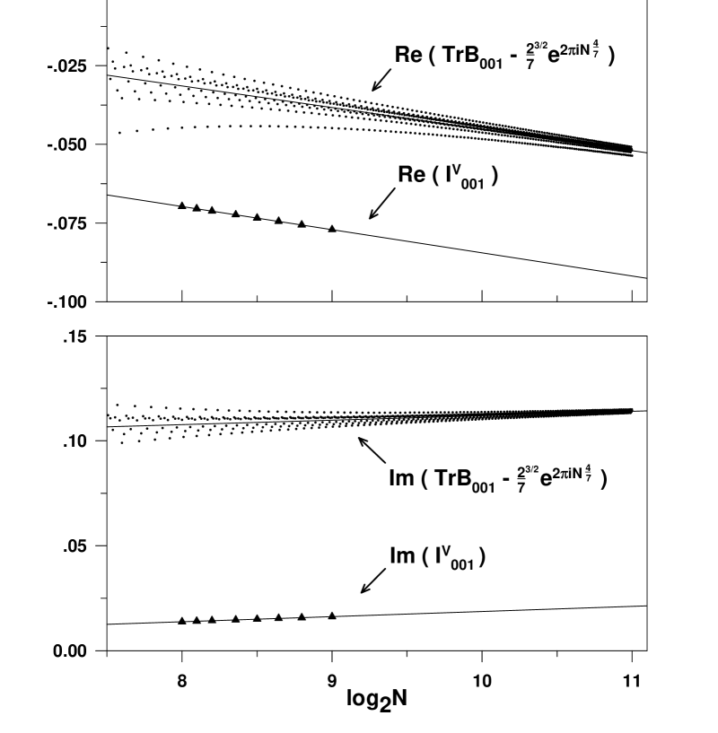
Figure 2: The exact trace $\mbox{Tr}B_{(0,0,1)}$ as a function of $\log_{2}N$ (the Gutzwiller term has been substracted) together with the corresponding vertex integral $I_{(0,0,1)}^{V}$.

Figure 4: Integration domains. Non–decreasing contributions to the first trace of the map arise from integrating the phase $e^{-2\pi iNp_{1}q_{0}}$ over the shaded squares. The square containing the origin (a stationary point of the first kind) provides the $\log N$ term plus a constant one. The correct constant term is obtained when the contributions from all the squares lying along the axes (they contain an infinity of second kind stationary points) are added up. Several lines of constant phase have been drawn for reference.

Table 1: Anomalous contributions to the trace from each family of paths with a common symbol $\epsilon$. Displayed are the complex coefficients $a_{\mbox{\scriptsize\boldmath$\epsilon$}}$ of the $\log N$ terms in the asymptotic expansion of the three shortest traces. Exact results were obtained by explicit numerical calculation of the partial traces. ”Theory” means the result of evaluating the vertex Poisson integral. For times 1–2 the integrals are done analytically, for $L=3$ numerically. In the numerical cases, a linear fit has been done to extract the coefficients (See e.g. Figs. 2, 3). The square brackets contain the estimated maximum error in the least significative figure.

$L$	$\epsilon$	$a_{\mbox{\scriptsize\boldmath$\epsilon$}}$ (exact)	$a_{\mbox{\scriptsize\boldmath$\epsilon$}}$ (theory)
1	$(0)$	$(0,-0.2251[1])$	$-i\frac{\sqrt{2}}{2\pi}\approx(0,-0.22508)$
2	$(0,0)$	$(-0.0234[2],-0.106[1])$	$-\frac{\log 2}{3\pi^{2}}-\frac{i}{3\pi}\approx(-0.02341,-0.1061)$
2	$(1,0)$	$(-0.0232[2],0.0001[2])$	$-\frac{\log 2}{3\pi^{2}}\approx(-0.02341,0)$
3	$(0,0,0)$	$(-0.0313[3],-0.0609[5])$	$(-0.0318[3],-0.0607[2])$
3	$(0,0,1)$	$(-0.01055[10],0.00350[5])$	$(-0.01064[1],0.00352[3])$

References

- [1] H. M. Nussenzveig, Diffraction Effects in Semiclassical Scattering (Cambridge University Press, Cambridge, 1992).
- [2] P. W. O’Connor and S. Tomsovic, Ann. Phys. (NY) 207 (1991) 218-264.
- [3] M. Saraceno and A. Voros, Physica D 79 (1994) 206-268.
- [4] A. Lakshminarayan, Ann. Phys. (NY) 239 (1995) 272-295.
- [5] M. G. E. da Luz and A. M. Ozorio de Almeida, Nonlinearity 8 (1995) 43–64.
- [6] M. Saraceno, Ann. Phys. (NY) 199 (1990) 37–60.
- [7] A. M. Ozorio de Almeida and M. Saraceno, Ann. Phys. (NY) 210 (1991) 1-15.
- [8] N. L. Balazs and A. Voros, Ann. Phys. (NY) 190 (1989) 1-31.
- [9] L. Mandel and E. Wolf, Optical coherence and quantum optics (Cambridge, New York, 1995); N. G. Van Kampen, Physica 14 (1949), 575.
- [10] F. Toscano, The traces of the baker’s map–Trabajos de Seminario (Universidad de Buenos Aires, Buenos Aires, 1995) (unpublished, in spanish).
- [11] J. H. Hannay, J. P. Keating and A. M. Ozorio de Almeida, Nonlinearity 7 (1994) 1327-1342 .
- [12] M. Abramowicz and I. A. Stegun, Handbook of Mathematical Functions (Dover, New York, 1972).
- [13] I. S. Gradshteyn and I. M. Ryzhik, Tables of Integrals, Series and Products (Academic, New York, 1980).