Characteristic Spatial Scales in Earthquake Data

Abstract

We present a new technique in order to quantify the dynamics of spatially extended systems. Using a test on the existence of unstable periodic orbits, we identify intermediate spatial scales, wherein the dynamics is characterized by maximum nontrivial determinism. This method is applied to earthquake catalogues containing time, coordinates and magnitude. As a result we extract a set of areas with significant deterministic and low–dimensional dynamics from the data. Finally, a simple model is used to show that these scales can be interpreted as local spatial coupling strengths.

PACS number(s): 05.45.+b,64.60.Lx,91.30.Dk

]

I Introduction

In recent years a lot of techniques to analyse single complex time series have been developed (cf. [1]). But a special challenge is the analysis of spatiotemporal dynamics, especially of natural systems. Although such systems become more and more important, e.g. in environmental research [2] or brain imaging techniques [3], little is known about how to analyse the corresponding data. Mostly the spatial extension is not taken into account and the more–dimensional data are simplified to one–dimensional time series [4]. This may be senseful for systems, which behave approximately homogeneously in space, but in general this assumption is not fulfilled for natural systems. As a consequence much information is lost after the modification of the data, e.g. by describing a complex spatial pattern by a single number like a mean value or a variance or a more complicated parameter like a fractal dimension. More dynamical approaches are based on a decomposition of spatiotemporal patterns into special basis functions, e.g. wavelet transformation [5] or the Karhunen–Loève method [6]. But these techniques are not appropriate in the case of rather irregular and noisy data.

The purpose of this contribution is to search for characteristic spatial scales, on which the interesting dynamical properties of the system can be observed. This idea allows to take the spatial extension of a system into account and is applicable to a large variety of data. Analysing the dynamics on these scales will give a maximum of nonlinear and low–dimensional determinism [7]. As a result the underlying dynamics can be represented locally by a vector in a low–dimensional space. This idea was suggested by Rand and Wilson [8] for systems, where the global dynamics is in a steady state and, therefore, trivial in the thermodynamic limit. Most natural systems, however, are far from thermodynamic equilibrium [9] and their system size is far from infinite size. As a consequence, we observe complex dynamical behavior even on the largest observable scales. Therefore, the concept of Rand and Wilson has to be modified for the analysis of this class of systems.

On small scales the dynamics is dominated by intrinsic stochasticity and on large scales spatial averaging over dynamically desynchronized parts of the system suppresses determinism as well as stochastic fluctuations. Therefore, the averaging procedure itself may be exploited for the analysis of spatiotemporal time series. We search for intermediate scales, where, on the one hand a deterministic signal is observed and on the other hand the loss of dynamical information arising from spatial averaging is as small as possible. To identify such a nontrivial determinism, we use a formalism of Pei and Moss [7] based on the existence of unstable periodic orbits.

As a dynamically rich and interesting subject, we apply this approach to natural seismicity which provides a lot of chaotic and fractal features, because the underlying processes like stress accumulation and ruptures are strongly nonlinear (cf.  [10, 11]). Here we mention the famous Gutenberg–Richter law [13]

$$logN=am+b,$$ (1)

where $N$ is the number of earthquakes with magnitude greater than or equal to $m$. The magnitude $m$ is related to the seismic energy $E$ by

$$logE=cm+d$$ (2)

with constants $a$, $b$, $c$ and $d$. Inserting Eq. (2) into Eq. (1) a power–law for the density function $D(E)$ is obtained

$$D(E)=\frac{dN}{dE}=\frac{a}{c}\ 10^{\ b-\frac{ad}{c}}\ E^{\ \frac{a}{c}-1}=C\ E^{\tau}.$$ (3)

In general power–laws with noninteger exponent $\tau$ indicate fractal distributions [11].

Due to technical difficulties, the analysis of earthquake data is not straightforward. These data are point–like and not equidistant in time and space, of course. Furthermore most catalogues are not complete in the sense that they contain all micro–quakes. In the next section we describe a pre–processing of the catalogue in order to generate regular data. In Sec. III we give the algorithm for the extraction of the scales. This algorithm is applied in Sec. IV to the real data and in Sec. V to the model data. Finally, we summarize the main ideas and results of our work.

II Data and Pre–processing

The data, which are investigated here incorporate 10.779 earthquakes recorded in Armenia between 1974 and 1994 [12]. Each earthquake is described by a four–dimensional vector consisting of time, longitude, latitude and magnitude. The events are distributed very complex, i.e. not equidistant, in time and space. For the data analysis it is helpful to handle with data, which are at least equidistant in time. Therefore, we subdivide the time into intervals $T_{i}=i\cdot\Delta t$ and the space into cells $A_{j}$ where the local dynamics is considered; the shape of the spatial cells will be determined in the next section. Corresponding to Eq. (2) we introduce the total energy $E_{ij}$ in this cell by

$$E_{ij}=\sum\limits_{t\in T_{i},\vec{x}\in A_{j}}10^{m(\vec{x},t)}.$$ (4)

For simplicity we have defined $c=1$ and $d=0$ for the constants in Eq. (2). Now we can define an effective magnitude $M_{ij}$ as a continuous function of time and space by

$$M_{ij}=logE_{ij}.$$ (5)

The subdivision into cells has to be chosen fine enough so that the loss of dynamical information is as small as possible.

For a fixed spatial area $A$ around a point $\vec{x}_{f}=$ (latitude,longitude) we compute the function

$$\sigma_{A,\vec{x}_{f}}(t)=\int\limits_{0}^{t}\ \left(M_{A,\vec{x}_{f}}(t^{\prime})-{\overline{M}_{A,\vec{x}_{f}}}\right)\ dt^{\prime},$$ (6)

where ${\overline{M}_{A,\vec{x}_{f}}}$ is a sliding temporal mean of $M_{A,\vec{x}_{f}}(t)$. We have found that $500$ time intervals (corresponding to an interval length of 15 days) and a window length of $100$ for the sliding mean are appropriate values for our calculations. In Fig. 1 we show the spatial distribution of seismic activity $\Sigma_{j}$ integrated over the whole time $[0,t_{max}]$

$$\Sigma_{j}=\log\int\limits_{0}^{t_{max}}\ \sum\limits_{\vec{x}\in A_{j}}10^{m(\vec{x},t)}\ dt.$$ (7)

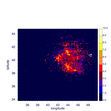
FIG. 1.: Spatial distribution of seismic activity (colour coded).

III Characteristic Spatial Scales

The challenge here is to include the spatial extension of the system in the analysis of the earthquake data. For this aim we want to extract spatial regions from the data, wherein the dynamics is highly deterministic. In contrast to global descriptions, where the spatial extension is simplified to a number, much less dynamical information is lost then.

The main idea is to search for deterministic dynamics in time series $\sigma_{A_{j},\vec{x}}(t)$ corresponding to a fixed point $\vec{x}$ and different areas $A_{j}$.

We call a scale characteristic, if the dynamics in one area is deterministic with higher significance than in the other ones. The time series $\sigma_{A,\vec{x}}(t)$ corresponding to this scale is then the appropriate choice for further investigations of the local dynamics. In our calculations we use circles with increasing radius for these areas.

We describe now the procedure for the extraction of characteristic scales in four steps:

1. Scatter plot of the time series $\{\sigma_{n}\}$:
   For the scatter plot we choose an embedding of $\{\sigma_{n}\}$:

   $$f(\sigma_{n})=\sigma_{n+k}.$$ (8)

   The lag $k$ is determined by the condition that the auto–correlation of the time series is sufficiently small. This is fulfilled for $k=4$.

2. Detecting candidates for unstable periodic orbits (UPOs):
   The identification of unstable periodic orbits [7, 14] rests on the occurrence of a special sequence of points in the time series. If the system’s trajectory enters such a sequence, an UPO is visited by following a predictable pattern of values of the time series. An UPO is an intersection point of a stable and an unstable manifold [7]. In the vicinity of an UPO, we can approximate these manifolds locally linear. We define the following criteria for an UPO candidate (see Fig. 2): (1) the UPO itself is close to the line of identity: the perpendicular distance to the line of identity is smaller than the mean of the perpendicular distances of the five points and (2) a straight line approaches the line of identity (stable manifold) and a straight line diverges from the line of identity (unstable manifold). We want to point out that these conditions are only capable to detect candidates for UPOs in time series, because they are necessary but not sufficient ones. We refer to [15] for a method which is more appropriate to detect UPOs itself.

   

   FIG. 2.: Visual definition of an UPO candidate in a time series $x(n)$: the dots are the data points, the squares denote the characteristic sequence of points (1,2,3: stable direction; 3,4,5: unstable direction), point 3 is the UPO candidate which is close to the line of identity (dotted line).

3. Definition of the statistical significance:
   The statistical significance for the number of UPOs can be defined by comparing the original data with a large number of surrogate data files. Therefore, we count the number of UPOs in the original data, $N,$ and in the surrogate data, $N_{s},$ and compute the statistical significance [7]:

   $$K=\frac{N-\langle N_{s}\rangle}{\sigma_{s}},$$ (9)

   where $\sigma_{s}$ is the standard deviation of $N_{s}$ and $\langle N_{s}\rangle$ the mean value of $N_{s}$ over all surrogate data files. For Gaussian distributions $K\geq 3$ is equivalent to a confidence level of $99\%$ to reject the null hypothesis that the original data are linear in the sense that they do not contain a significant number of UPO candidates. Our surrogate data are generated by phase randomization and amplitude adjustment of the original data [16]. This guarantees that the auto–correlation function as well as the distribution of the data are conserved.

4. Extraction of characteristic scales:
   The procedure to extract the characteristic scales from the data works as follows: One point in space is surrounded by circles with increasing radius: $r=\Delta r,\ 2\Delta r,\ \dots\$. The step width is chosen to $\Delta r=5$ km. For each circle a time series $\sigma_{n}$ is generated from the data as described in Sec. II. In these time series we detect the UPO candidates and compute the significance $K(r)$ in comparison with $100$ surrogate data files. A characteristic scale around a point $\vec{x}$ with radius $r_{max}$ and significance $K_{max}$ is given, if (1) $K(r_{max})\geq 3$ and (2) $K(r_{max})=K_{max}=\max\limits_{r}K(r)$. This procedure is applied to each point of a $20\times 20$ lattice. To avoid finite size effects we exclude boundary points in space. Note also that the number of events in the boundary regions is too small to provide reliable results.

We have checked that the results do not depend sensitively on the parameters.

IV Results of data analysis

Applying our algorithm to the earthquake data exhibits indeed in some regions such characteristic scales. Two examples are shown in Fig. 3, where we have plotted the significance $K$ from Eq. (9) as a function of the spatial scale represented by an index for two fixed points in space. In Fig. 3(a) we observe values for $K$ up to six and a clear maximum for the scale index 15. Here it is possible to assign a characteristic scale to the point $\vec{x}$. In contrast to this we cannot find such a significant scale in Fig. 3(b). The level of $K=3$ is not reached here. Note that the significances in Fig. 3(a) and  3(b) are quite different, although the points $\vec{x}$ are very close in space. This result underlines that an averaging over the whole space or large parts of the space is indeed questionable.

However, the rule for the extraction of the characteristic scale is rather simple. Not for all points a clear maximum of the significance can be observed. In some cases there are two or more maxima, or the shape of the curve $K(r)$ is approximately constant. For the investigation of the local dynamics the function $K$ should be studied in detail. But as a global approach, the rules for the selection of the scales seem to be reasonable.

FIG. 3.: Significance $K$ as a function of the spatial scale for two points in space: (a) $\vec{x}=(40.3,41.8),$ (b) $\vec{x}=(41.4,43.7).$ A unit of the scale index is 5 km.

The distribution of the scales in space is given in Fig. 4. The scale sizes are related to the general seismic activity (see Fig. 1); the dynamics in very active regions is mostly determined on small scales, whereas in regions with less activity larger scales dominate. It is important to check, if this relationship is linear. In this case the distribution of the scales would simply reflect the seismic activity given in Fig. 1 and the results were completely trivial. This is, in fact, not the case, because the linear correlation coefficient between these quantities is almost zero.

Our technique uses unstable periodic orbits to quantify nonlinear determinism. Next we check, whether a simpler discriminating statistic can be used for this aim. Therefore, we perform the same algorithm to obtain the time series (Eq. (6)), and compute then the skewness [16] of these series instead of numbers of UPO candidates. The skewness is a rather simple quantity, which indicates nonlinear behavior and time reversal invariance in time series. Comparing original data and surrogate data by Eq. (9), no significant deviation is observed. As a consequence, we need indeed a more powerful method to detect nonlinear features in the dynamics.

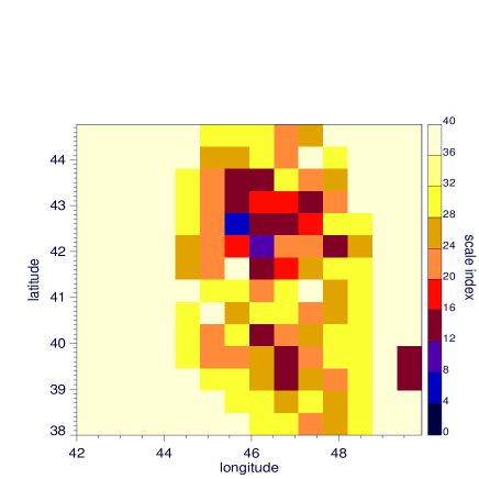
FIG. 4.: Distribution of characteristic scales in space (colour coded); a unit of the scale index is 5 km.

V Calculations with model data

To connect our results of data analysis with physical properties of the system, we want to apply our technique also to standard models of seismicity. In this way we can control the properties of the simulated data by changing some parameters of the model.

An important point is the incompleteness of the earthquake catalogue, which may have influence on the results. For instance the Gutenberg–Richter law is only fulfilled for $2\leq m\leq 6$ (see Fig.  5). In the region $m>6$ the number of events is too small to provide a good statistics and for $m<2$ a large number of micro–quakes is not measured for this catalogue. To analyse the dependence of the significance of UPOs on the completeness of the data, we generate a synthetic earthquake catalogue and assume that these surrogate earthquake data behave similar to the real data.

FIG. 5.: The Gutenberg–Richter law (Eq. (1)): the points denote the number of earthquakes with magnitude greater or equal to $m$, the dashed line is a linear fit for $2\leq m\leq 6.$

There is a standard model for earthquakes by Bak and Tang [17] exhibiting self–organized criticality. This is a cellular automaton analogue to well–known stick–slip–models [18], which describes the earth’s crust to be in a stationary critical state so that the distribution of earthquakes follows the Gutenberg–Richter relation. For a detailed description of the model we refer to [17]. Here we only recall the rules for the redistribution of energy $Z(i,j)$, if a cell $(i,j)$ is in a critical state, i.e. $Z(i,j)>Z_{crit}$ :

$$Z(i,j)\longrightarrow Z(i,j)-4$$ (10)

$$Z(i\pm 1,j\pm 1)\longrightarrow Z(i\pm 1,j\pm 1)+1$$ (11)

With a $50\times 50$–grid and the critical value $Z_{crit}=3$ we create two earthquake catalogues: (A) a “complete” catalogue including all micro–quakes and (B) a “truncated” one, where quakes with $E<10$ ($m<1$) are discarded. We choose the size of (2) equal to that of the real data. In Fig. 6 we compare the results of (A) and (B) for one point in space; like in Fig. 3 we compute the significance from Eq. (9) for UPOs as a function of the scale size. The shapes of the curves are very similar and the scales with hints for determinism are in almost all cases the same or at least very close to each other. Furthermore we see that this simple model yields scales with relatively high significances. While the dynamics for small scales is rather stochastic and provides only small significances, we observe the most deterministic behavior for intermediate scales. For large scales the significance decreases again due to averaging effects in the dynamics, but does not tend to zero.

However, in contrast to the real earthquake data the model is nearly homogeneous in space. For more realistic models one could add a component in Eq. (10), which is space–dependent.

FIG. 6.: Significance $K$ as a function of the spatial scale for the point $\vec{x}=(17,18)$ in the model of Bak and Tang; solid line: truncated model catalogue, dashed line: complete model catalogue.

In the following we study another modification of the model, which yields a physical interpretation of the characteristic scales. Considering models with global coupling forces (e.g. slider–block–models), the size of the scale should increase with growing coupling. To proof this for our model, we introduce a coupling strength $C$ by changing the rules for the energy release. If $Z(i,j)>Z_{crit}$, the redistribution of the energy follows now

$$Z(i,j)\longrightarrow 0$$ (12)

$$Z(i\pm 1,j\pm 1)\longrightarrow Z(i\pm 1,j\pm 1)+(1-\epsilon)\frac{Z(i,j)}{4}$$ (13)

so that an increasing value of $\epsilon$ corresponds to a decreasing coupling strength $C:=1-\epsilon$. Note that $Z$ is noninteger here in contrast to the model in [17]. Moreover, a cell in a critical state decays by transferring its total energy to the neighbor cells. This modification is done in order to produce a large magnitude spectrum. In the model with integer energy units, the number of different magnitudes decreases very fast with decreasing coupling. For different couplings we compute the total number of UPO candidates and compare it with 30 surrogate earthquake catalogues that are generated by randomizing the original catalogue such that the distribution is conserved. For one scale the mean number of UPO candidates is computed. In Fig. 7(a) we show the statistical significance from Eq. (9) for three different couplings $C$. We observe a significant deviation between the model data and the mean of the surrogate data for intermediate scales. For small and large scales no significant determinism is present due to the statistics and averaging effects. Although the model is driven by stochastic forces, the dynamics behaves deterministic on certain scales. More important is the dependence of these scales on the coupling: for strong couplings we observe still positive significances on large scales; in contrast to this, the significance decreases very fast in this scale range for small couplings. On Fig. 7(b) the results for the calculation with the real data are given, which shows a qualitatively good agreement with the model with strong coupling in Fig. 7(a).

FIG. 7.: (a) shows the significance for UPOs depending on the scale for three different couplings in the model described in the text (Eq. 12). For each scale the average number (over space) of UPOs is compared with 30 surrogate earthquake catalogues. The definition of the significance is analogue to Eq. (9). One curve belongs to one catalogue. (b) results from the same calculation for the Armenia catalogue. A unit of the scale index is 10 km.

Due to these results from pure model studies, we get indications that large spatial scales in real earthquake data correspond to strong coupling forces in the earth’s crust.

VI Summary and Outlook

We have presented a new technique to characterize the dynamics of spatially extended natural systems. In particular, we have analysed earthquake catalogues, but in principle the method can be regarded as a part of a general approach for data analysis, because it is applicable to a large variety of systems.

The main idea is to check whether it exists an intermediate spatial scale between the noisy micro-scales and the large scales, where the dynamics is dominated by averaging effects. This intermediate scale is then characterized by a maximum of nontrivial determinism and it represents the appropriate length scale, on which the main features of the underlying dynamics can be observed. To extract the characteristic spatial scale from the data, we look for unstable periodic orbits in time series corresponding to different scales. The occurrence of such orbits is a measure for nonlinear and low–dimensional determinism. The scale with the highest significance (with respect to the condition $K\geq 3$) – in comparison with surrogate data – can be considered as the characteristic scale.

Our calculations show that intermediate scales with deterministic dynamics in the sense as mentioned above exist in earthquake data. In some spatial regions we observe a clear maximum for the significance as a function of the scale size. Moreover, in some regions the statistical significance reaches values up to seven.

An interesting result arising from studies with model data is the interpretation of the spatial scales. Using a modification of the well–known model of Bak and Tang, we have shown that the scale is related to a coupling strength, i.e. high coupling strengths correspond to large scales. This seems to be an interesting tool to evaluate models, in particular such with locally varying coupling forces.

However, one has to keep in mind that our ansatz is still very general and should be refined for special applications. For instance some effects of seismicity are not yet included in our approach. Perhaps the technique can be improved by using more complicated areas than circles. This would be well–adapted for the study of spatial inhomogeneities. In this context it is a special challenge to analyse the influence of such inhomogeneities in simple models.

In the future we should focus on a detailed analysis of the time series. From seismology we know that every main shock is more or less accompanied by precursery phenomena [20] and aftershocks [19]. It is an interesting question, if the occurrence of UPOs in the time series can be connected with these patterns.

We believe, however, that our technique is promising for the analysis of a large variety of spatially extended natural systems.

REFERENCES

- [1] P. Grassberger, T. Schreiber, C. Schaffrath, Intern. J. Bif. Chaos 1, 521 (1991); M. Casdagli et al., in Applied Chaos, edited by J. H. Kim and J. Stringer (John Wiley & Sons, New York, 1992) p. 335; E. Ott et al., Coping with Chaos (John Wiley & Sons, New York, 1994).
- [2] M. P. Hassell, H. N. Comins, R. M. May, Nature 370, 290 (1994); M. A. Nowak, R. M. May, Nature 359, 826 (1992).
- [3] M. Hämäläinen et al., Rev. Mod. Phys. 65, 414 (1993).
- [4] G. Rossi, in Fractals and Dynamic Systems in Geoscience, edited by J. H. Kruhl (Springer, Berlin, 1994) p. 169.
- [5] C. K. Chui, An Introduction to Wavelets (Academic Press, Boston, 1992).
- [6] R. Friedrich, C. Uhl, in Evolution of Dynamical Structures in Complex Systems (Springer, Berlin, 1992) p. 251.
- [7] X. Pei, F. Moss, Nature 379, 618 (1996).
- [8] D. A. Rand, H. B. Wilson, Proc. R. Soc. Lond. B 259, 111 (1995).
- [9] H. Haken, Synergetics (Springer, Berlin, 1977).
- [10] R. Meissner, in Fractals and Dynamic Systems in Geoscience, edited by J. H. Kruhl (Springer, Berlin, 1994) p. 159.
- [11] D. L. Turcotte, Fractals and chaos in geology and geophysics (Cambridge University Press, 1992).
- [12] Armenia Earthquake Catalogue, unpublished (GeoForschungsZentrum Potsdam, 1994).
- [13] B. Gutenberg, C. F. Richter, Ann. Geofis. 9, 1 (1956).
- [14] S. J. Schiff et al., Nature 370, 615 (1994).
- [15] P. So et al., Phys. Rev. Lett. 76, 4705 (1996).
- [16] J. Theiler et al., Physica D 58, 77 (1992); J. Theiler et al., in Nonlinear Modeling and Forecasting. SFI Studies in the Sciences of Complexity, edited by M. Casdagli, S. Eubank (Proc. Vol. XII, Addison Wesley, 1992) p. 163.
- [17] P. Bak, C. Tang, J. Geophys. Res. 94, 15635 (1989); P. Bak, C. Tang, K. Wiesenfeld, Phys. Rev. A38, 364 (1988).
- [18] R. Burridge, L. Knopoff, Seis. Soc. Am. Bull. 57, 341 (1967); L. Knopoff, J. A. Landoni, M. S. Ambinante, Phys. Rev. A 46, 7445 (1992).
- [19] G. M. Molchan et al., Phys. Earth Planet Int. 61, 128 (1990).
- [20] S. Schreider, Phys. Earth Planet Int. 61, 113 (1990).