Wound-up phase turbulence in the Complex Ginzburg-Landau Equation

Abstract

We consider phase turbulent regimes with nonzero winding number in the one-dimensional Complex Ginzburg-Landau equation. We find that phase turbulent states with winding number larger than a critical one are only transients and decay to states within a range of allowed winding numbers. The analogy with the Eckhaus instability for non-turbulent waves is stressed. The transition from phase to defect turbulence is interpreted as an ergodicity breaking transition which occurs when the range of allowed winding numbers vanishes. We explain the states reached at long times in terms of three basic states, namely quasiperiodic states, frozen turbulence states, and riding turbulence states. Justification and some insight into them is obtained from an analysis of a phase equation for nonzero winding number: rigidly moving solutions of this equation, which correspond to quasiperiodic and frozen turbulence states, are understood in terms of periodic and chaotic solutions of an associated system of ordinary differential equations. A short report of some of our results has been published in [Montagne et al., Phys. Rev. Lett. 77, 267 (1996)].

I Introduction

A The complex Ginzburg-Landau equation and its phase diagram

Spatio-temporal complex dynamics [1, 2, 3] is one of the present focus of research in nonlinear phenomena. This subject lies at the intersection of two important lines of thought: on the one hand the generalization of the ideas of dynamical systems theory to high dimensional situations[4, 5, 6], and on the other the application of some concepts and tools developed in the field of statistical mechanics, specially in the study of phase transitions, to the analysis of complex nonequilibrium systems [7, 8, 9].

An important effort has been devoted to the characterization of different dynamical states and transitions among them for model equations such as the Complex Ginzburg-Landau Equation (CGLE) [1, 4, 7, 10, 11, 12, 13, 14, 15, 16, 17]. The CGLE is an equation for a complex field $A({\bf x},t)$:

$$\partial_{t}A=A+(1+{\it i}c_{1})\nabla^{2}A-(1+{\it i}c_{2})\mid A\mid^{2}A\ .$$ (1)

$A({\bf x},t)$ represents the slowly varying, in space and time, complex amplitude of the Fourier mode of zero wavenumber when it has become unstable through a Hopf bifurcation (the signs used in (1) assume it to be supercritical). The CGLE is obtained universally when analyzing the dynamics sufficiently close to the bifurcation point. In one dimensional geometries, (1) or a coupled set of similar equations with additional group velocity terms describe also the evolution of the amplitudes of Hopf-bifurcated traveling waves [1, 14, 18]. Binary fluid convection [19], transversally extended lasers [20, 21], chemical turbulence[22, 23], bluff body wakes [24], the motion of bars in the bed of rivers [25], and many other systems have been described by the CGLE in the appropriate parameter range. We will restrict ourselves in this paper to the one-dimensional case, that is $A=A(x,t)$, with $x\in[0,L]$. As usual, we will use periodic boundary conditions in $x$.

The one-dimensional Eq. (1) has traveling wave (TW) solutions

$$A_{k}=\sqrt{1-k^{2}}e^{i(kx-\omega_{k}t)},\ \omega_{k}=c_{2}+(c_{1}-c_{2})k^{2}$$ (2)

with $k\in[-1,1]$. When $1+c_{1}c_{2}>0$ there is a range of wavenumbers $[-k_{E},k_{E}]$ such that TW solutions with wavenumber in this range are linearly stable. Waves with $k$ outside this range display a sideband instability (the Eckhaus instability [1, 13, 26]). The limit of this range, $k_{E}$, vanishes as the quantity $1+c_{1}c_{2}$ approaches zero, so that the range of stable traveling waves vanishes by decreasing $1+c_{1}c_{2}$. The line $1+c_{1}c_{2}=0$, is the Benjamin–Feir–Newell line[27, 28], labeled BFN in Fig.1. Above that line, where $1+c_{1}c_{2}<0$, no traveling wave is stable and different turbulent states exist. A major step towards the analysis of phases and phase transitions in (1) was the numerical construction in [7, 11, 12] of a phase diagram that shows which type of regular or chaotic behavior occurs in different regions of the parameter space $[c_{1},c_{2}]$. Fig. 1 has been constructed from the data in [7, 11, 12]. Above the BFN line, three types of turbulent behavior are found, namely phase turbulence (PT), defect or amplitude turbulence (DT), and bichaos (BC).

FIG. 1.: Regions of the parameter space $[c_{1},c_{2}]$ for the CGLE displaying different kinds of regular and chaotic behavior. Lines $L_{1},L_{3}$ were determined in[7, 11, 12]. See the text in Section II for the explanation of the different symbols.

Phase turbulence is a state in which $A(x,t)=|A|e^{i\varphi}$ evolves irregularly but with its modulus always far from $|A|=0$. Since the modulus never vanishes, periodic boundary conditions enforce the winding number defined as

$$\nu\equiv\frac{1}{2\pi}\int_{0}^{L}\partial_{x}\varphi dx$$ (3)

to be a constant of motion, fixed by the initial condition. $\nu$ is always an integer because of periodic boundary conditions . The quantity $\bar{k}\equiv 2\pi\nu/L$ can be thought of as an average or global wavenumber. To the left of line $L_{1}$ (region DT), in contrast, the modulus of $A$ becomes zero at some instants and places (called defects or phase slips). In such places the phase $\varphi$ becomes undefined, so allowing $\nu$ to change its value during evolution. BC is a region in which either PT, DT, or spatial coexistence of both can be observed depending on initial conditions. It should be noted that chaotic states exist also below the BFN line: To the left of the line $L_{2}$, a chaotic attractor called Spatio Temporal Intermittency (STI) coexists with the stable traveling waves [11]. A diagram qualitatively similar to Fig. 1 has also been found for the two-dimensional CGLE [29, 30]. Despite the relevance of $\nu$ in the dynamics of the CGLE, most studies of the PT regime have only considered in detail the case of $\nu=0$. In fact the phase diagram in Fig. 1 was constructed [7, 11, 12] using initial conditions that enforce $\nu=0$. Apart from some limited observations[12, 13, 30], systematic consideration of the $\nu\neq 0$ (wound) disordered phases has started only recently [10, 31, 32]. States with $\nu\neq 0$ are precisely the subject of the present paper.

B The PT-DT transition

Among the regimes described above, the transition between PT and DT has received special attention [7, 10, 16, 31, 32, 33]. The PT regime is robustly observed for the large but finite sizes and for the long but finite observation times allowed by computer simulation, with the transition to DT appearing at a quite well defined line ($L_{1}$ in Fig. 1) [15, 30], but it is unknown if the PT state would persist in the thermodynamic limit $L\rightarrow\infty$. One possible scenario is that in a system large enough, and after waiting enough time, a defect would appear somewhere, making thus the conservation of $\nu$ only an approximate rule. In this scenario, a PT state is a long lived metastable state. In the alternative scenario, the one in which PT and the transition to DT persist even in the thermodynamic limit, this transition would be a kind of ergodicity breaking transition [10, 34] in which the system restricts its dynamics to the small portion of configuration space characterized by a particular $\nu$. DT would correspond to a “disordered” phase and different “ordered” phases in the PT region would be classified by its value of $\nu$. The idea of using a quantity related to $\nu$ as an order parameter [10] has also been independently proposed in [31].

The question of which of the scenarios above is the appropriate one is not yet settled. Recent investigations seem to slightly favor the first possibility [12, 15, 16, 30]. The most powerful method in equilibrium statistical mechanics to distinguish true phase transitions from sharp crossovers is the careful analysis of finite-size effects [35]. Such type of analysis has been carried out in [15, 30] , giving some evidence (although not definitive) that the PT state will not properly exist in an infinite system or, equivalently, that the $L_{1}$ line in Fig. 1 approaches the BFN line as $L\rightarrow\infty$. Here we present another finite-size scaling analysis, preliminarily commented in [10], based on the quantity $\nu$ as an order parameter. Our result is inconclusive, perhaps slightly favoring the vanishing of PT at large system sizes. In any case, the PT regime is clearly observed in the largest systems considered and its characterization is of relevance for experimental systems, that are always finite. In this paper we characterize this PT regime in a finite system as we now outline.

C Outline of the paper

We show that in the PT regime there is an instability such that a conservation law for the winding number occurs only for $\nu$ within a finite range that depends on the point in parameter space. PT states with too large $|\nu|$ are only transients and decay to states within a band of allowed winding numbers. Our results, presented in Section II, allow a characterization of the transition from PT to DT in terms of the range of conserved $\nu$: as one moves in parameter space, within the PT regime and towards the DT regime, this range becomes smaller. The transition is identified with the line in parameter space at which such stable range vanishes. Analogies with known aspects of the Eckhaus and the Benjamin-Feir instabilities are stressed. States with $\nu\neq 0$ found in the PT region of parameters at late times are of several types, and Section III describes them in terms of three [10] elementary wound states. Section IV gives some insight into the states numerically obtained by explaining them in terms of solutions of a phase equation. In addition, theoretical predictions are made for such states. The paper is closed with some final remarks. An Appendix explains our numerical method.

II The winding number instability

The dynamics of states with non-zero winding number and periodic boundary conditions has been studied numerically in the PT region of parameters. In order to do so we have performed numerical integrations of Eq. (1) in a number of points, shown in Fig. 1. Points marked as $\Diamond$ correspond to parameter values where intensive statistics has been performed. The points overmarked with $\times$ correspond to places where finite-size scaling was analyzed. Finally the symbol $+$ correspond to runs made in order to determine accurately the PT-DT transition line ($L_{1}$). Our pseudospectral integration method is described in the Appendix. Unless otherwise stated, system size is $L=512$ and the spatial resolution is typically 512 modes, with some runs performed with up to 4096 modes to confirm the results. The initial condition is a traveling wave, with a desired initial winding number $\nu_{i}$, slightly perturbed by a random noise of amplitude $\epsilon$. By this amplitude we specifically mean that a set of uncorrelated Gaussian numbers of zero mean and variance $\epsilon^{2}$ was generated, one number for each collocation point in the numerical lattice. Only results for $\nu_{i}>0$ are shown here. The behavior for $\nu_{i}<0$ is completely symmetrical.

The initial evolution is well described by the linear stability analysis around the traveling wave [13, 14, 36, 26]. Typically, as seen from the evolution of the power spectrum, unstable sidebands initially grow. This growth stops when an intense competition among modes close to the initial wave and to the broad sidebands is established. Configurations during this early nonlinear regime are similar to the ones that would be called riding turbulence and described in Section III. At long times the system approaches one of several possible dynamical states. In general, they can be understood in terms of three of them, which are called basic states. In the next section these final states are discussed. When the initial winding number is above a critical value $\nu_{c}$, which depends on $c_{1}$ and $c_{2}$, there is a transient period between the early competition and the final state during which the winding number changes.

In Fig. 2a we show in grey levels the phase $\varphi(x,t)$ for a given run with parameters $c_{1}=2.1$ and $c_{2}=-0.6$. The space-time defects appear as dislocations in this representation. In Fig. 2b the winding number has been plotted as a function of time. The winding number changes from the initial value $\nu_{i}=20$ to the final value $\nu_{f}=14$. The discrete jumps in $\nu$ are due to the integer nature of this quantity, and they are smeared out when averages over several realizations are performed. The resemblance with the dynamics of the Eckhaus instability of regular waves is striking. In fact, since the changes in $\nu$ occur on top of a chaotic wave, the analogy is stronger with the Eckhaus instability in the presence of stochastic fluctuations [37, 38]. In the latter case a local wavenumber independent of position cannot be defined because of noise, while for phase turbulent waves the disorder is generated by the system dynamics. Nevertheless in both cases the configurations can be characterized by a global wavenumber such as $\bar{k}$ or $\nu$. The analogy is also instructive since it can be shown [38, 39] that for the one–dimensional relaxational dynamics considered in [37, 38, 39] (which is related to Eq.(1) with $c_{1}=c_{2}=0$) there is no long range order in the system, so that there is no proper phase transition in the thermodynamic $L\rightarrow\infty$ limit. Despite this, for large but finite sizes and long but finite times, sharp transitions are observed and critical exponents and scaling functions can be consistently introduced [37]. This example should make clear that even in the case that the PT-DT transition would not exist in the thermodynamic limit, its characterization in large finite systems is justified. The development of phase slips from PT waves of high enough $\nu_{i}$ can be viewed as a kind of Eckhaus-like instability for turbulent waves, whereas the usual Eckhaus instability [13] appears for regular waves. This similarity was one of the main motivations for the kind of analysis that follows.

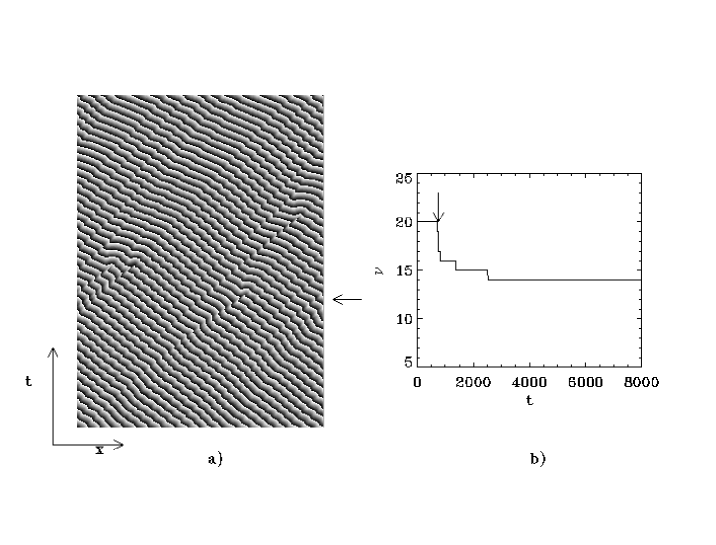
FIG. 2.: a) Spatiotemporal evolution of the phase $\varphi(x,t)$ coded in grey levels with time running upwards and $x$ in the horizontal direction. The lighter grey correspond $\varphi(x,t)=-\pi$ and darker to $\varphi(x,t)=\pi$. The time interval shown in the picture goes from $t=500$ to $1000$ time units of a total run of $10^{4}$. $c_{1}=2.1$, $c_{2}=-0.60$, and the initial condition was a TW with $\nu_{i}=20$ that decayed to $\nu_{f}=14$. The arrow indicates the time at which $\nu$ begins to change. b) The complete time evolution of the winding number for this initial condition.

For each point in parameter space and initial winding number considered, we have averaged over 50 independent random realizations of the white Gaussian perturbation added to the initial wave. Figs. 3a and 3b show the temporal evolution of this average $\bar{\nu}(t)$ and its variance $\sigma$ for $c_{1}=2.1$ and $c_{2}=-0.83$. Four values of the initial winding number ($\nu_{i}=10,15,20,25$) are shown. Typically, the curve $\bar{\nu}(t)$ decays from $\nu_{i}$ to a final winding number $\nu_{f}$.  

FIG. 3.: a) Temporal evolution of $\bar{\nu}(t)$ for four different initial winding numbers $\nu_{i}=25$ (solid), $20$(dotted), $15$ (dashed) $10$ (dashed-dotted). $c_{1}=2.1,c_{2}=-0.83$ (PT regime). b) Winding number standard deviation $\sigma$.

The variance displays the behavior typical of a decay from a unstable state [40], namely a pronounced maximum at the time of fastest variation of $\bar{\nu}(t)$. The final value of $\sigma$ gives the dispersion in the final values of the winding numbers. Although the behavior shown in Fig. 3 is very similar to the observed in [37] for a stochastic relaxational case, the scaling laws found there do not apply here. The main qualitative difference is that in a range of $\nu_{i}$ the sign of the average final $\bar{\nu}$ is here opposite to the initial one. In addition for some of the initial winding numbers (i.e. $\nu_{i}=20$ in Fig. 3) $\bar{\nu}(t)$ is not monotonously decaying, showing a small recovery after the fast decrease in $\bar{\nu}$. These features are also observed for other values of $[c_{1},c_{2}]$, so that figure 3 is typical for $[c_{1},c_{2}]$ in the PT region of Fig. 1. For comparison we show $\bar{\nu}(t)$ and its variance in Fig. 4 for the point $c_{1}=1.6$ and $c_{2}=-1.0$, in the “bichaos” region. The main difference is the existence of fast fluctuations in $\bar{\nu}$ and $\sigma$. They are related to the characteristic dynamics of the bichaos regime: The final state depends on the initial conditions and it can correspond to PT, DT or even coexistence of both. In the 50 realizations performed all these possibilities were found. When DT appears, there are big fluctuations of the winding number around $\nu=0$ that produce the wiggling on the averaged value. More than 50 realizations should be performed to smooth out such big fluctuations.

FIG. 4.: a) Temporal evolution of $\bar{\nu}(t)$ for an initial winding number of $\nu_{i}=4$ in the bichaos regime. $c_{1}=1.6,c_{2}=-1.0$. b) Winding number standard deviation $\sigma$.

Returning to the PT parameter regime (Fig. 3) the decay of the initial state is seen to take place during a characteristic time which depends on $\nu_{i}$. We quantify this time $\tau$ as the time for which half of the jump in $\nu$ is attained. $\tau$ increases as $\nu_{i}$ decreases, and there is a critical value of $\nu_{i}$, $\nu_{c}$, such that no decay is observed for $\nu_{i}<\nu_{c}$. Then $\tau$ diverges (critical slowing down) when $\nu_{i}$ approaches $\nu_{c}$ from above. This gives a sensible procedure to determine $\nu_{c}$: Figs. 5a and 5b show $1/\tau$ as a function of $\nu_{i}$. In Fig. 5a, $c_{1}$ is fixed and the different symbols correspond to different values of $c_{2}$. In Fig. 5b, $c_{2}$ is fixed and the symbols correspond to different values of $c_{1}$. The values of $\nu_{c}$ have been estimated by extrapolating to $1/\tau=0$ a linear fit to the points of smallest $\nu_{i}$ in each sequence. Motivated by [37] we have tried to fit the divergence of $\tau$ with nontrivial critical exponents, but we have found no significant improvement over the simpler linear fit. The values of $\nu_{c}$ so obtained are plotted in the insets of Figs. 5a and 5b. The range of conserved winding numbers $[-\nu_{c},\nu_{c}]$ is analogous to the Eckhaus range of stable wavenumbers when working below the BFN line. $\nu_{c}$ can also be obtained by directly determining the value of $\nu_{i}$ below which $\nu(t)$ does not change in any of the realizations. This method can only give integer values of $\nu_{c}$ whereas the method based on $\tau$ gives a real number which is preferable when looking for continuous dependences of $\nu_{c}$ on system parameters. The two methods however give consistent results within the discretization indeterminacy.

                

FIG. 5.: a) Inverse of the characteristic time for winding number relaxation as a function of the initial winding number. The value of $c_{1}$ is fixed ($c_{1}=2.1$) and $c_{2}$ varies from near the BFN line ($c_{2}\simeq-0.48$) to the $L_{1}$ line ($c_{2}\approx-0.9$). Different symbols correspond to $c_{2}=-0.6$ ($+$), $c_{2}=-0.7$ ($\ast$), $c_{2}=-0.75$ ($\Diamond$), $c_{2}=-0.8$ ($\triangle$), $c_{2}=-0.83$ ($\Box$). The inset shows the critical winding number ($\nu_{c}$) as a function of $c_{2}$. b) Idem but the value of $c_{2}$ is fixed ($c_{2}=-0.83$) and $c_{1}$ varies from near the BFN line ($c_{1}\simeq 1.33$) to $c_{1}=2.5$ . Different symbols correspond to $c_{1}=1.6$ ($+$), $c_{1}=1.8$ ($\ast$), $c_{1}=1.96$ ($\Diamond$), $c_{1}=2.1$ ($\triangle$), $c_{1}=2.3$ ($\Box$), $c_{1}=2.5$ ($\times$). The inset shows the critical winding number ($\nu_{c}$) as a function of $c_{1}$

The insets of Fig. 5a and Fig. 5b indicate a clear decrease in $\nu_{c}$ as the values of $c_{1}$ and $c_{2}$ approach the $L_{1}$ line. In fact we know that $\nu_{c}$ should be zero to the left of $L_{1}$, since no wave maintains its winding number constant there. This lead us to a sensible method for determining the position of line $L_{1}$ [10], alternative to the one based in the density of defects used in [7]. It consists in extrapolating the behavior of $\nu_{c}$ to $\nu_{c}=0$. A simple linear fit has been used. The same method to determine the line $L_{1}$ has been independently introduced in [31, 32]. The coefficients of the linear fit are not universal: they depend of the particular path by which the line $L_{1}$ is approached. With this method the line $L_{1}$ is determined as the line at which the range of conserved winding numbers $[-\nu_{c},\nu_{c}]$ shrinks to zero. The analogy with the Eckhaus instability of regular waves is again remarkable: in the same way as the range of Eckhaus-stable wavenumbers shrinks to zero when approaching the BFN line from below, the allowed $\nu$ range shrinks to zero when approaching the $L_{1}$ line from the right. The difference is that below the BFN line the values of the wavenumber characterizes plane-wave attractors, whereas above that line, $\nu$ characterizes phase-turbulent waves. In this picture, the transition line PT–DT appears as the BFN line associated to an Eckhaus-like instability for phase turbulent waves. For the case of Fig. 5a the PT–DT transition is located at $c_{1}=2.1,c_{2}=-0.89\pm 0.02$, and $c_{1}=2.60\pm 0.02,c_{2}=-0.83$ for the case of Fig. 5b. The agreement with the position of the line as determined by [7, 12], where system sizes similar to ours are used, is good. For example for $c_{1}=2.1$ their value for $L_{1}$ is $c_{2}=-0.92$. The points marked as $+$ in Fig. 1 correspond to runs used to determine the position of the transition line $L_{1}$ directly as the line at which defects appear in a long run even with $\nu=0$. All these ways of determining $L_{1}$ give consistent results. Below the point $P$, $\nu_{c}$ goes to zero when the parameters approach the line $L_{3}$, not $L_{1}$, thus confirming the known behavior that below point $P$ in Fig. 1 the line separating phase turbulence from defect turbulence when coming from the PT side is actually $L_{3}$.

The use of a linear fit to locate the line $L_{1}$ is questionable and more complex fits have been tested. However, the simplest linear fit has been found of enough quality for most of the the situations checked. Clearly some theoretical guide is needed to suggest alternative functional forms for $\nu_{c}(c_{1},c_{2})$. We notice that the analogous quantity below the BFN line, the Eckhaus wavenumber limit, behaves as $q_{E}\sim\sqrt{\epsilon}$ for small $\epsilon$, being $\epsilon$ the difference between either $c_{1}$ or $c_{2}$ and its value at the BFN line. From the insets in Figs. 5a or 5b, this functional form is clearly less adequate than the linear fit used.

Another interesting point to study is the dependence of the final average winding number $\bar{\nu}_{f}$ on the initial one $\nu_{i}$. Fig. 6 shows an example using $c_{1}=2.1$ and $c_{2}=-0.8$. The behavior for other values of the parameters is qualitatively similar. $\bar{\nu}_{f}$ remains equal to the initial value if $\nu_{i}\leq 5$ during the whole simulation time, so that $\nu_{c}\approx 5$, a value consistent with the one obtained from the divergence of $\tau$ and plotted in the inset of Fig. 5a. For $\nu_{i}>\nu_{c}$, the final winding number is always smaller than the initial one. By increasing $\nu_{i}$ a minimum on $\bar{\nu}_{f}$ is always observed, and then $\bar{\nu}_{f}$ tends to a constant value. Figure 6 also shows the winding number associated with one of the two Fourier modes of fastest growth obtained from the linear stability analysis of the initial traveling wave. The one shown is the lowest, the other one starts at $\bar{\nu}_{f}=28$ and grows further up. Obviously they do not determine the final state in a direct way. This is consistent with the observation mentioned above that the winding number instability does not develop directly from the linear instability of the traveling wave, but from a later nonlinear competition regime.

FIG. 6.: The final averaged winding number ($\bar{\nu}_{f}$) as a function of the initial one $\nu_{i}$. The initial condition is a TW with winding number $\nu_{i}$ for $c_{1}=2.1\mbox{ and }c_{2}=-0.8$. The dashed line corresponds to the lowest of the two Fourier modes of fastest growth in the linear regime as a function of $\nu_{i}$.

As stated in the introduction, a powerful way of distinguishing true phase transitions from effective ones is the analysis of finite-size scaling [35]. We have tried to analyze size–effects from the point of view of $\nu$ as an order parameter. In the DT state such kind of analysis was performed in [41]. Egolf showed that the distribution of the values taken by the ever-changing winding number is a Gaussian function of width proportional to $\sqrt{L}$. This is exactly the expected behavior for order parameters in disordered phases. In the thermodynamic limit the intensive version of the order parameter, $\nu/L$, would tend to zero so that the disordered DT phase in the thermodynamic limit is characterized by a vanishing intensive order parameter. For the PT states to be true distinct phases, the existence of a nonvanishing $\nu_{c}$ such that $\nu$ is constant for $|\nu|<\nu_{c}$ is not enough. The range of stable winding numbers should also grow at least linearly with $L$ for this range to have any macroscopic significance. The analysis of the growth of $\nu_{c}$ with system size has been performed in points $c_{1}=2.1,c_{2}=-0.8\mbox{ and }c_{1}=1.96,c_{2}=-0.83$ of parameter space. $\nu_{c}$, determined as explained before, is plotted in Fig. 7 for several system sizes for which the statistical sample of 50 runs was collected for each $\nu_{i}$.  

FIG. 7.: The critical winding number ($\nu_{c}$) as a function of the length $L$ of the system is shown. Different symbols correspond to $c_{1}=2.1\mbox{ and }c_{2}=-0.8$ ($\triangle$), and $c_{1}=1.96,\mbox{ and }c_{2}=-0.83$ ($\Diamond$). The straight lines are linear fits to the two sets of data.

There is a clear increasing, close to linear, of $\nu_{c}$ as a function of $L$, thus indicating that for this range of system sizes the range of allowed winding numbers is an extensive quantity and then each $\nu$ is a good order parameter for classifying well defined PT phases. It should be noted however that for the larger system size for which extensive statistics was collected ($L=2048$) data seem to show a tendency towards saturation. Thus our study should be considered as not conclusive, and larger systems sizes need to be considered.

III Different asymptotic states in the PT region

Typical configurations of the PT state of zero winding number consist of pulses in the modulus $|A|$, acting as phase sinks, that travel and collide rather irregularly on top of the $k=0$ unstable background wave (that is, a uniform oscillation)[7, 12]. The phase of these configurations strongly resembles solutions of the Kuramoto-Shivashinsky (KS) equation. Quantitative agreement has been found between the phase of the $\nu=0$ PT states of the CGLE and solutions of the KS equation near the BFN line[16].

For states with $\nu\neq 0$ a typical state[12] is the one in which an average speed (in a direction determined by the sign of $\nu$) is added to the irregular motion of the pulses. We have found that in addition to these configurations there are other attractors in the PT region of parameters. We have identified [10] three basic types of asymptotic states for $\nu\neq 0$, which we describe below. Other states can be described in terms of these basic ones. Except when explicitly stated, all the configurations described in this Section have been obtained by running for long times Eq. (1) with the initial conditions described before, that is small random Gaussian noise added to an unstable traveling wave. The winding number of these final states is constant and is reached after a transient period in which the winding number might have changed.

Figs. 8, 9 and 11 show examples of the basic states that we call riding PT (Fig. 8), quasiperiodic states (Fig. 9) and frozen turbulence (Fig. 11). For each figure: Panel (a) corresponds to a grey scale space–time plot of $\partial_{x}\varphi(x,t)$. Panel (b) shows the value of this quantity and the modulus of the field $(\mid A\mid)$ as a function of position at the time indicated by an arrow in panels (a) and (d). Panel (c) shows the spatial power spectrum $S(q,t)$ of $A(x,t)$ for the same time. Finally, panel (d) shows the quantity $W=\int\mid\partial_{t}S(q,t)\mid dq$, which is a global measure of the temporal change in the spatial power spectrum.

Riding PT. This state (see Fig. 8) is the most familiar one [12]: wiggling pulses in the gradient of the phase with a systematic drift in a direction determined by $\nu$. The modulus of the field consists of a disordered spatial sequence of small pulses and shocks, with $A(x,t)$ always far from zero. The spatial power spectrum $S(q)$ has a peak corresponding to the global wave number $\bar{k}$ (associated in this case with $\nu=-1$, so that $\bar{k}=2\pi\nu/L=-0.012$) and a broad background associated with the turbulent motion “riding” on the traveling wave. The time evolution of $W$ shows a decay towards a fluctuating non-zero value, indicating that the power spectrum is continuously changing in time as corresponds to the turbulent state reached by the system.

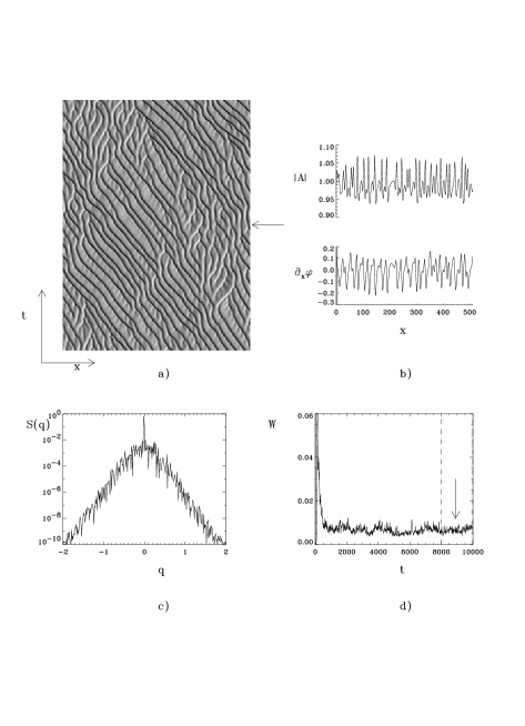
FIG. 8.: a) Spatiotemporal evolution of $\partial_{x}\varphi(x,t)$. The lighter grey correspond to the maximum value of $\partial_{x}\varphi(x,t)$ and darker to the minimum. Last $2000$ time units of a run $10^{4}$ time units long for a riding PT state at $c_{1}=2.1$ , and $c_{2}=-0.83$. The initial condition was a TW with $\nu_{i}=20$ that decayed to $\nu_{f}=-1$ after a short time. b) A snapshot of $\mid A(x,t)\mid\mbox{ and }\partial_{x}\varphi(x,t)$ as a function of $x$ for $t=8900$ which is indicated by an arrow in a) and d). c) Spatial power spectrum $S(q)$ as a function of wavenumber at the same time $t=8900$. d)The time evolution of the quantity $W$ defined in the text. The dashed line indicates the initial time for picture a).

Quasiperiodic states. These states (an example is shown in Fig. 9) can be described as the motion of equidistant pulses in the gradient of the phase that travel at constant speed on top of the background wave. The fact that the periodicity of the pulses and that of the supporting wave are not the same justify the name of quasiperiodic. We show later that these states correspond to the ones described in Ref. [13]. In Fig. 9a, the modulus $\mid A\mid$ and the gradient of the phase clearly exhibit uniformly traveling pulses. The spatial power spectrum $S(q)$ (Fig. 9c) clearly shows the quasiperiodic nature of this state: a central peak, corresponding to the dominant traveling wave, with equally spaced peaks surrounding it, showing the periodicity of the pulses. The peaks are not sharp because this configuration has been obtained from a random perturbation. The decrease of $W$ in Fig. 9d indicates that the peaks are narrowing. Its asymptotic approach to zero indicates that the amplitudes of the main modes reach a steady value and $S(q)$ becomes time independent.

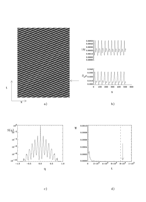
FIG. 9.: Same as in Fig. 8 but for last $35000$ time units of a run $10^{5}$ time units long for a quasiperiodic state. The initial condition is random noise with an amplitude of $0.05$. $c_{1}=2.0$ , and $c_{2}=-0.8$. b) and c) correspond to a time $t=8\times 10^{4}$.

More perfect quasiperiodic configurations can be obtained from initial configurations that are already quasiperiodic. Figure 10 shows the quantity $W$ for a state generated at $c_{1}=2.1\mbox{ and }c_{2}=-0.6$ from an initial traveling wave with a sinusoidal perturbation. The initial traveling wave had $\nu_{i}=18$ and the winding number of the sinusoidal perturbation was $\nu=22$. The travelling wave decayed to a state with $\nu_{f}=10$ of the quasiperiodic type, cleaner than before. The spatial power spectrum (shown in the inset at the time indicated by an arrow in the main picture) shows the typical characteristics of a quasiperiodic state.  

FIG. 10.: a)The time evolution of $W$ for a quasiperiodic state. The initial condition is a TW sinusoidally perturbed for $c_{1}=2.1\mbox{ and }c_{2}=-0.6$ . In the inset the spatial power spectrum $S(q)$ as a function of wavenumber at the time $t=8900$ indicated by an arrow in the main picture.

Frozen turbulence. This state (see Fig. 11) was first described in [10]. It consists of pulses in $\partial_{x}\varphi$ traveling at constant speed on a traveling wave background, as in the quasiperiodic case, but now the pulses are not equidistant from each other (see Fig. 11b). The power spectrum at a given time is quite different from the one of a quasiperiodic state. It is similar, instead, to the power spectrum obtained in the riding PT state: $S(q)$ is a broad spectrum in the sense that the inverse of the width, which gives a measure of the correlation length, is small compared with the system size. Here however $W$ relaxes to zero, so that the power spectrum finally stops changing (thereby the name frozen).

FIG. 11.: Same as in Fig. 9 but for last $2500$ time units of a run $10^{4}$ time units long for a frozen turbulence state. The initial condition was a TW of $\nu_{i}=12$ that decayed to $\nu_{f}=6$ after a short time. $c_{1}=1.75$ and $c_{2}=-0.8$. The time of b) and c) is $t=8900$, indicated by an arrow as in previous figures.

This behavior is an indicator of the fact [10], obvious from Fig. 11, that the pattern approaches a state of rigid motion for the modulation in modulus and gradient of the phase of the unstable background plane wave. That is, the field $A(x,t)$ is of the form:

$$A(x,t)=g(x-vt)e^{i\left(kx-\omega_{k}t+\alpha(t)\right)}$$ (4)

where $g$ is a uniformly translating complex modulation factor. It is easy to see that configurations of the form (4) have a time-independent spatial power spectrum. Torcini [31] noticed in addition that the function $\alpha(t)$ is linear in $t$ so that the solutions are in fact of the form

$$A(x,t)=f(x-vt)e^{i(kx-\omega t)}$$ (5)

where again $f(x-vt)$ is a complex valued function and $\omega$ can differ from $\omega_{k}$. $f$ and $g$ differ only in a constant phase. The envelopes $g(x-vt)$ or $f(x-vt)$ turn out to be rather irregular functions in the present frozen turbulence case, whereas they are periodic in the quasiperiodic configurations discussed above.

After presenting the basic states, we continue addressing some interesting mixed states that can be described in terms of them. Most of the configurations ending up in the frozen turbulence or in the quasiperiodic states have long time transients of the riding turbulence type. Only at long times a decay to rigid propagation occurs. There are cases in which a different type of decay happens. For example Fig. 12 shows a case in which the system jumps from a very strong riding turbulence regime to another state, also of the riding turbulence type, but much more regular. The quantity $W$, shown in Fig. 12b, turns out to be a valuable tool in distinguishing the different regimes: a superficial look at Fig. 12a could be easily misunderstood as indicating the approach of the system towards a frozen turbulence state, but the lack of decay towards zero of $W$ identifies the final state as riding turbulence. The arrows indicate the jump to the second state. Fig. 13 shows a state characterized by a recurrence between two different riding turbulence states, showing a kind of temporal intermittency.

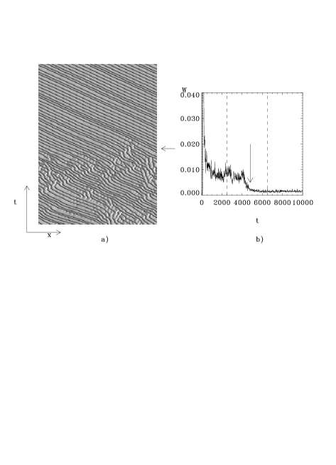
FIG. 12.: a) Spatiotemporal evolution of $\partial_{x}\varphi(x,t)$ for a riding turbulence state that decays onto another one. $c_{1}=2.5$, $c_{2}=-0.75$. The initial condition was a TW of $\nu_{i}=20$ that decayed to $\nu_{f}=-2$ in a short time. b) Time evolution of $W$. The dashed lines indicate the time interval shown in a) (from $t_{1}=2500$ to $t_{2}=6500$ of a run $10^{5}$ time units long). The arrow indicates the transition from one of the riding turbulence regimes to the other one.

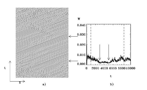
FIG. 13.: a) Spatiotemporal evolution of $\partial_{x}\varphi(x,t)$ showing intermittency between riding turbulence states. $c_{1}=2.1$, $c_{2}=-0.83$. The initial condition is a TW of $\nu_{i}=1$ that did not change. b)Time evolution of $W$. The dashed lines indicate the time interval shown in a) (from $t_{1}=1000$ to $t_{2}=8500$ of a run $10^{4}$ time units long). The arrows indicate the end of a riding turbulence regime and the beginning of another one.

Finally Fig. 14 shows a riding turbulence state with zero winding number. This is not however a typical configuration, since usually for $\nu=0$ there is no preferred direction for the pulses to drift, whereas the figure shows that in fact there is a local drift at some places of the system. It turns out that this state can be understood as composed by two domains of different local winding number: $\nu=1$ and $\nu=-1$, so that globally $\nu=0$. The pulses travel either in one direction or in the other depending of the region of the system in which they are. In Fig. 14b a snapshot of the gradient of the phase $\partial_{x}\varphi(x,t)$ and the phase itself $\varphi(x,t)$ is shown. Lines showing the average trend in the phase are plotted over the phase, clearly identifying the two regions in the system. This coexistence of the different basic states at different places of space, or at different times as in Fig. 13, was already mentioned in [11] where it was argued to give rise to a kind of spatio-temporal intermittent behavior.

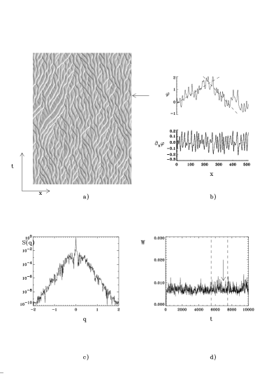
FIG. 14.: a) Spatiotemporal evolution of $\partial_{x}\varphi(x,t)$. The time interval corresponds to $5500\mbox{ to }7500$ time units of a run $10^{4}$ time units long for a riding PT state at $c_{1}=2.1$ and $c_{2}=-0.83$. The initial condition was a TW with $\nu_{i}=0$ that did not change. b) Snapshots of $\varphi(x,t)\mbox{ and }\partial_{x}\varphi(x,t)$ as a function of $x$ at the time $t=6980$ indicated by an arrow in a) and d). The dashed lines in the graph of $\varphi(x,t)$ indicate average slopes, that is “local” wavenumbers. c) Spatial power spectrum $S(q)$ as a function of wavenumber at the same time $t=6980$. d)Time evolution of $W$. Dashed lines indicate the time interval of picture a).

Given the large variety of configurations that are observed, and the very long transients before a jump from one state to another occurs, it would be difficult to conclude from numerical evidence alone that the three kinds of states considered as basic above are true asymptotic states. Some analytical insight would be desirable to be sure that these three states are attractors of the dynamics. The next Section is devoted to provide such analytical justification.

IV Asymptotic states in terms of the phase dynamics

The question on whether it is possible or not to describe the PT regime of the CGLE from a closed equation for the phase alone has been posed by several authors[15, 16, 30, 42, 43]. A phase equation is obtained by considering a long wavelength perturbation of a plane-wave solution in the CGLE (1). It is clear that this phase equation will only describe phase dynamics close to the homogeneous plane-wave (that is the one with $\nu=0$) if the perturbation is made around the spatially–homogeneous solution. In order to get a description of PT at $\nu\neq 0$ the expansion should be done for a perturbation on a traveling wave solution with wavenumber ($k$) different from zero,

$$A=(\sqrt{1-k^{2}}\,+a(x,t))e^{i\left(kx+\phi(x,t)\right)}\;,$$ (6)

Here $k$ is taken as $k=\frac{2\pi}{L}\nu$. If $A$ satisfies periodic boundary conditions the same conditions apply to $\phi$ because any global phase winding is included in $k$ (the total phase is $\varphi=kx+\phi$). From general symmetry arguments the general phase equation for $k\neq 0$ should read, up to fourth order in gradients:

$$\partial_{t}\phi = \Omega_{0}-v_{g}\partial_{x}\phi-D_{2}\partial_{x}^{2}\phi+D_{11}(\partial_{x}\phi)^{2}+D_{3}\partial_{x}^{3}\phi+D_{12}(\partial_{x}\phi)(\partial_{x}^{2}\phi)$$ (7)

$$- D_{4}\partial_{x}^{4}\phi+D_{13}(\partial_{x}\phi)(\partial_{x}^{3}\phi)+D_{22}\left(\partial_{x}^{2}\phi\right)^{2}+D_{112}(\partial_{x}\phi)^{2}(\partial_{x}^{2}\phi)+\ldots\;.$$ (8)

When $v_{g}=D_{3}=D_{12}=D_{13}=D_{22}=D_{112}=0$, Eq. (8) reduces to the Kuramoto–Sivashinsky (KS) equation [44, 45] that is the lowest order nonlinear phase equation for the case $k=0$. For $k\neq 0$, Eq. (8) was systematically derived up to third order in gradients in [36]. An easy way of obtaining the values of all the coefficients in (8) was discussed in [46]: First, $\Omega_{0}$ is related to the frequency of the plane-wave solutions:

$$\Omega_{0}=-\omega_{k}=-c_{2}-(c_{1}-c_{2})k^{2}$$ (9)

Second, the linear terms can be obtained from the eigenvalue $\lambda(k,q)$ corresponding to the phase-like branch in the linear stability analysis of the wave of wavenumber $k$ with respect to perturbations of wavenumber $q$[13, 14, 36, 26]:

$$\lambda(k,q)=-iv_{g}q+D_{2}q^{2}-iD_{3}q^{3}-D_{4}q^{4}+{\cal O}(q^{5})$$ (10)

with

$$v_{g} = 2k(c_{1}-c_{2})$$ (11)

$$D_{2} = -(1+c_{1}c_{2})+{2k^{2}(1+c_{2}^{2})\over 1-k^{2}}$$ (12)

$$D_{3} = {2k(1+c_{2}^{2})\left[-c_{1}+(c_{1}+2c_{2})k^{2}\right]\over\left(1-k^{2}\right)^{2}}$$ (13)

$$D_{4} = \frac{1}{2\left(1-k^{2}\right)^{3}}\left\{c_{1}^{2}(1+c_{2}^{2})-2k^{2}(1+c_{2}^{2})(c_{1}^{2}+6c_{1}c_{2})\right.$$ (14)

$$+ k^{4}\left.\left[4+(1+c_{2}^{2})(c_{1}^{2}+12c_{1}c_{2})+c_{2}^{2}(24+20c_{2}^{2})\right]\right\}\;.$$ (15)

Third, the nonlinear terms can be obtained from the following consistency relationship: If (6) is an exact solution of the CGLE, then $\phi(x,t)$ satisfies the phase equation with coefficients depending on $k$. In addition if $(\sqrt{1-k_{1}^{2}}+a_{1}(x,t))e^{i(k_{1}x+\phi_{1}(x,t))}$ is another exact solution of the CGLE, then $\phi_{1}(x,t)$ satisfies a similar phase equation but with coefficients depending on $k_{1}$ instead of $k$. But this solution can be written as $(\sqrt{1-k_{1}^{2}}+a_{1}(x,t))e^{i(kx+(k_{1}-k)x+\phi_{1}(x,t))}$ so that $(k_{1}-k)x+\phi_{1}(x,t)$ is also solution of the phase equation with coefficients depending on $k$ (with different boundary conditions). By combining the two equations satisfied by $\phi_{1}$ and expanding the coefficients depending on $k_{1}$ as a power series around $k$ (assuming $k_{1}-k$ small) the following relationships between linear and nonlinear terms are obtained:

$$D_{11}=-{1\over 2}{\partial v_{g}\over\partial k}\ ,\ \ \ D_{12}=-{\partial D_{2}\over\partial k}\ ,\ \ \ D_{13}={\partial D_{3}\over\partial k}\ ,\ \ \ D_{112}=-{1\over 2}{\partial^{2}D_{2}\over\partial k^{2}}$$ (16)

So that

$$D_{11} = c_{2}-c_{1}$$ (17)

$$D_{12} = -{4k(1+c_{2}^{2})\over\left(1-k^{2}\right)^{2}}$$ (18)

$$D_{13} = {2(1+c_{2}^{2})\over\left(1-k^{2}\right)^{3}}\left[-c_{1}+6c_{2}k^{2}+(2c_{2}+c_{1})k^{4}\right]$$ (19)

$$D_{112} = -{2(1+c_{2}^{2})(3k^{2}+1)\over\left(1-k^{2}\right)^{3}}$$ (20)

The coefficient $D_{22}$ is only obtained following the method to higher order in $(k_{1}-k)$. The coefficients up to third order in gradients can be found also in [36] and approximate expressions for them are given in [13].

The traveling wave of wavenumber $k$ becomes unstable when the coefficient $D_{2}$ becomes positive. One expects that the first terms in the gradient expansion (8) give a good description of the phase dynamics in the weakly nonlinear regime, that is $D_{2}$ positive but small (note that for a given $k\neq 0$ this includes part of the region below the BFN line in Fig 1). The arguments presented in [46] imply that the relative importance of the different terms in a multiple scale expansion in which $D_{2}$ is the small parameter can be established by considering $\phi\sim\partial_{x}\sim D_{2}^{1/2}$. Then the dominant terms close to the instability of wave $k$ are the ones containing $\Omega_{0}$ and $v_{g}$. After them, the terms with coefficients $D_{3}$ and $D_{11}$ are the most relevant. Up to this order Eq. (8 ) is a Korteweg–de Vries equation (KdV). The terms with $D_{2}$, $D_{4}$ and $D_{12}$ appear at the next order. The importance of the terms in $D_{2}$ and $D_{4}$ for a qualitatively correct description of phase dynamics is obvious since they control the stability properties of the wave of wavenumber $k$. The importance of the term with coefficient $D_{12}$ was stressed in [13, 47]: if it is large enough it can change the character of the bifurcation from supercritical to subcritical.

The detailed comparison of the reduced dynamics (8) with the complete CGLE phase dynamics is beyond the scope of the present paper. The aim of this Section is to use Eq.(8) just to get some understanding of the asymptotic states presented in Section III. To this end we will use the detailed results available from the work of Chang et al. [48]. These results are obtained for the so-called Kawahara equation [49, 50, 47, 48, 51] which is Eq.(8) with $D_{12}=D_{13}=D_{22}=D_{112}=0$. The term $D_{12}$, which according to Kuramoto estimations [46] is of the same order for small $D_{2}$ as the terms in $D_{2}$ and $D_{4}$, will thus be neglected. It would be certainly necessary to consider the modifications introduced by the term $D_{12}$ into the results of [48]. This will be briefly discussed at the end of this section. At this point it is interesting to note that, to our knowledge, the only quantitative comparison of the phase dynamics with $k\neq 0$ obtained from a phase equation and from CGLE is [31, 32]. But the phase equation used in these references is the one presented in [42], in which the nonlinear terms considered are only those with coefficients $D_{11}$ and $D_{13}$. In addition $D_{11},D_{13}$, and the coefficients of the linear terms are considered only up to first order in $k$. Despite these limitations, in particular the absence of the $D_{12}$ term, the phase equation is found to reproduce well the phase dynamics of the CGLE, an agreement that degrades when the term in $D_{13}$ is suppressed [52]. Clearly further work is needed to establish firmly the relevance of the different terms in (8)[53]. Our study will be restricted to the situation of [48] (that is $D_{12}=D_{22}=D_{13}=D_{112}=0$) since no study of comparable detail for a more complete equation is available in the literature.

The situation of interest here is the one in which the traveling waves are unstable against a finite band of wavenumbers, so that $D_{2},\ D_{4}>0$. Making the following changes of variables in (8) with $D_{12}=D_{22}=D_{13}=D_{112}=0$:

$$\chi = \sqrt{\frac{D_{2}}{D_{4}}}\left(x-v_{g}t\right)\;,$$ (21)

$$\tau = \frac{D_{2}^{2}}{D_{4}}t\;,$$ (22)

$$u(\chi,\tau) = -\frac{D_{11}D_{4}^{1/2}}{2D_{2}^{3/2}}\partial_{x}\phi(x,t)\;.$$ (23)

the Kawahara equation[49, 50, 47, 48, 51] is obtained

$$\partial_{\tau}u=-\partial^{2}_{\chi}u-4u\partial_{\chi}u-\delta\partial^{3}_{\chi}u-\partial^{4}_{\chi}u\;,$$ (24)

with

$$\delta=-\frac{D_{3}}{\sqrt{D_{2}D_{4}}}$$ (25)

Since $\phi$ is periodic in $x$, $u(\chi,t)$ is periodic in $\chi$. In addition $\int_{0}^{L}u(\chi,\tau)d\chi=0$. To have some intuition on the meaning of the parameter $\delta$, its expansion at small $k$ reads

$$\delta\approx 2\sqrt{2}\,k\,\,{\rm sign}\,(c_{1})\sqrt{\frac{1+c_{2}^{2}}{\mid 1+c_{1}c_{2}\mid}}+{\cal O}(k^{3})\;.$$ (26)

It should be noted that $\delta$ does not diverge at the BFN line, as the expansion (26) seems to suggest, but below it. From Eq. (25) it is clear that $\delta$ diverges where $D_{2}$ vanishes indicating that the corresponding traveling wave of wavenumber $k$ has become Eckhaus unstable.

The Kawahara equation (24) has been considered in the context of surface waves on fluid films falling down an inclined or vertical plane [54], and also as a simple generalization of the KS or the KdV equations [49, 50]. It has also been considered in the context of growth shapes [55]. It reduces to KS for $\delta=0$ (or equivalently for $k=0$) when written in the original variable $\varphi$.

Equation (24) has periodic, soliton-like, spatially-irregular, and spatio-temporally chaotic solutions. [49, 50, 51]. In fact, all of these solutions have been analytically shown to exist [48]. All of them except the isolated soliton-like solution [56] are stable in some parameter regimes [48]. These kinds of solutions should manifest themselves (provided the approximate phase description holds) in the time evolution of the phase gradient $\partial_{x}\varphi$ ($=k+\partial\phi$) of the solutions of the CGLE (1) in the PT regime. The analytical results in [48] thus provide a firm basis for true existence of the numerically observed states described in Section III.

The detailed bifurcation analysis in [48] also gives detailed predictions for the wound states of the CGLE, within the range of validity of the phase description. We will reproduce here some of the results in [48] and reinterpret them in terms of the gradient of the phase of CGLE solutions. Our interest is centered in the rigidly moving train of pulses ( frozen turbulence and quasiperiodic states) observed in several of the numerical simulations reported in Section III. They are of the form (5), and because of (23) we have

$$u(\chi,\tau)=H(\xi)\ ,$$ (27)

with $\xi=\chi-v\tau$, being $v$ the velocity of the train of pulses we want to describe in units of $\chi\mbox{ and }\tau$. The partial differential equation (24) is reduced to an ordinary differential equation (ODE) for $H(\xi)$:

$$H^{iv}+\delta H^{\prime\prime\prime}+H^{\prime\prime}+4HH^{\prime}-vH^{\prime}=0\;.$$ (28)

The primes denote differentiation with respect to $\xi$. After an integration:

$$H^{\prime\prime\prime}+\delta H^{\prime\prime}+H^{\prime}-vH+2H^{2}=Q\;.$$ (29)

$Q$ is fixed in a nontrivial way by the condition $\int Hd\xi=0$ which follows from our periodic boundary conditions. This third order ODE can be rewritten as a three-dimensional dynamical system:

$$u^{\prime}_{1} = u_{2}$$ (30)

$$u^{\prime}_{2} = u_{3}$$ (31)

$$u^{\prime}_{3} = cu_{1}-u_{2}-\delta u_{3}-2(u_{1})^{2}$$ (32)

with

$$u_{1}(\xi) = H(\chi)-\frac{v}{4}+\sqrt{\frac{c^{2}}{16}+\frac{Q}{2}}\;,$$ (33)

$$c = \sqrt{8Q+v^{2}}\;.$$ (34)

Different qualitative behaviors in phase space of the solutions of the dynamical system (32) are related to the shape of the solutions of (28) [57]. This is illustrated in Fig. 15.

FIG. 15.: Schematic relationship between trajectories of the dynamical system (32) in phase space (left column) and solutions $u(\chi,\tau)=H(\xi=\chi-v\tau)$ of equation (24) (right column). a1) Fixed point of (32), a2) uniform solution of (24) (traveling wave in the CGLE (1)). b1) Periodic solution (limit cycle) of (32), b2) periodic train solution of (24) (quasiperiodic solution of the CGLE (1)). c1) Homoclinic trajectory of (32), c2) single pulse of (24). d1) Chaotic trajectory of (32), d2) spatially irregular solution of (24) (frozen turbulence in the CGLE).

We stress that all the solutions of (28) represent uniformly translating solutions of (24). No information is given on more complicated solutions of (24). The left column of Fig. 15 shows the possible trajectories of the dynamical system (32) while the right column shows the corresponding solution of (29), or equivalently $u(\chi,\tau)=H(\xi=\chi-v\tau)$ in equation (24). For a fixed point in (32) (fig. 15a1) we get a homogeneous solution in (24) (fig. 15a2) and (via (23)) a traveling wave solution in the CGLE (1). For a periodic trajectory in (32) (fig. 15b1) we get a train of periodic pulses in the solution of (24) (fig. 15b2) and a quasiperiodic solution in CGLE (1). An homoclinic trajectory in (32) (fig. 15c1) corresponds to a single pulse solution in (24) (fig. 15c2). Finally for a chaotic trajectory in (32) (fig. 15d1) we have an irregular solution $H(\xi)$ that corresponds to a rigidly traveling spatially irregular solution of (24) (fig. 15d2). The chaotic solutions of (32) are of the Shil’nikov type [48]. This means that the disordered configurations $H(\xi)$ (and thus $u$ and $\partial_{x}\varphi$) consist on nearly identical pulses irregularly spaced. This corresponds to the state named frozen turbulence for solutions of the CGLE.

The detailed analysis of [48] is done on the one hand by following the sequence of bifurcations of the state in which $H$ is a constant and of the state in which $H$ is close to the KdV soliton (with adequate rescaling Eq. (24) reduces to the KdV in the limit $\delta\rightarrow\infty$). On the other hand the powerful global theorems of Shil’nikov and their generalizations [58, 59, 60, 61] are used to establish the structure of the solutions of (32). The results of [48] relevant to our purposes can be summarized as follows (they can be read-off from figure 3 of Ref. [48] ):

1. Periodic solutions of (32) exist for all values of $\delta$ provided $\mid c\mid>\mid\delta\mid$. They are organized in a variety of branches. Solutions in the same branch differ by their periodicity, and each branch ends in a different kind of solitary-wave solution (infinite spatial period). The shape of the different solitary wave solutions characterizes the different branches.

2. For $\mid\delta\mid\,\vbox{\hbox{$\buildrel\textstyle>\over{\sim}$}}\,1.1$ only one of the branches of periodic solutions (the main branch) remains.

3. Chaotic solutions to (32) exist only for $\mid\delta\mid\lesssim 0.84$.

In addition Chang et al. [48] obtained results also for the full equation (24), without the restriction to rigidly traveling waves. Their numerical and analytical results can be summarized as

1. Periodic solutions in the main branch with its wavenumber within a given range are linearly stable for all $\delta$. A more precise determination of the range of stable wavenumbers for large $\delta$ was performed in [47].

2. In addition to the periodic solutions there are also spatio-temporal chaotic attractors for all $\delta$.

3. If $\mid\delta\mid>1.1$ only two of these strange attractors remain. For $\mid\delta\mid>3$ their basin of attraction seems to be much smaller than the one of the periodic solutions.

Expression (25) with (11)-(20) gives the relation between $\delta$ and the parameters of the CGLE. $\mid\delta\mid=\infty$ corresponds in Fig. 1 to the line at which the wave of wavenumber $k$ becomes Eckhaus unstable. It is approximately parallel and below the BFN line. The other lines of constant $\delta$, for fixed $k$, are also approximately parallel to the BFN line, and decreasing $\mid\delta\mid$ corresponds to entering into the PT region and going deep into it. All these lines concentrate onto the BFN line as $k$ approaches zero: for $k=0$, $\delta=0$ except on the BFN line $1+c_{1}c_{2}=0$ where $\delta$ is undefined. We now rephrase the conclusions above in terms of the three basic asymptotic states of the CGLE in the PT regime. They will be valid as long as the phase description (24) remains accurate.

1. There are PT solutions of the quasiperiodic type for all values of the parameters (as long as the phase description remains valid). Bounds on their velocity can be in principle obtained, but this is nontrivial since $Q$ is only known in an implicit way.

2. Increasing $\mid\delta\mid$ by approaching the Eckhaus instability for a given $k$ ($D_{2}=0$), or by increasing the winding number reduces the variety of quasiperiodic solutions.

3. Frozen turbulence solutions exist only for $\mid\delta\mid\lesssim 0.84$, that is far enough from the line $D_{2}=0$ or for small enough winding number.

4. There are linearly stable solutions in the main quasiperiodic branch for all values of the parameters.

5. There are also riding turbulence attractors for all values of parameters.

6. For $\mid\delta\mid>3$, that is at high winding number or close enough to the line $D_{2}=0$ the quasiperiodic solutions have a basin of attraction larger than the riding turbulence ones.

A general feature of these conclusions is that the important quantity is $D_{2}$, that is the distance in parameter space from the line at which the $k$-wave became Eckhaus unstable. This line is below the BFN line for $k\neq 0$. Thus not only traveling waves, but also quasiperiodic, frozen turbulence, and riding turbulence attractors should exist below the BFN line for $k\neq 0$. In practice it is relatively easy to find quasiperiodic states below but close the BFN line, but we have been unable to find the other two states so far. The difficulty in finding riding turbulence states can be a consequence of the small range of winding numbers for which they are stable ($|\nu|=L|k|/(2\pi)<\nu_{c}$) so that the observability condition $\mid\delta\mid<3$ immediately brings us above the BFN line. Another possibility is that the instability of the $\nu=0$ plane-wave attractor at the BFN line has consequences of a global character beyond the validity of the phase description.

The above predictions imply that the more promising zone for obtaining quasiperiodic solutions starting from random perturbations on a traveling wave of given winding number is for parameter values close and above $D_{2}=0$, or for high winding number ($\mid\delta\mid>3$). In any case no frozen turbulence should be observed in that zone.

Some qualitative aspects of the conclusions above have been shown to be correct. In particular Torcini and collaborators [31, 32] have shown that the average maximal Lyapunov exponent, quantifying the proportion of initial conditions that fall into the spatio-temporal chaotic strange attractors, is a decreasing function of $\nu$.

Our numerical solutions also agree with the prediction that quasiperiodic solutions show up more easily for small $D_{2}$. However, their basin of attraction appears to be much smaller than the implied by the conclusions of the phase description since it is reached with very low probability from our initial conditions. This is specially true above the BFN line. The reason for this is probably the effect of the neglected term $D_{12}$, which is known to reduce the range of stable periodic solutions [47] and even to eliminate it by making the bifurcation subcritical [13]. Above the BFN line the attractor that we observe more frequently at high winding number from our initial conditions is the frozen turbulent state.

A more detailed checking of the predictions above would be desirable. This is however beyond the scope of the present paper since a detailed theoretical analysis of the global properties of the phase space for the equation containing the term $D_{12}$ would be probably needed beforehand. A promising alternative can be the study of the exact equation for $f(x-vt)$ in (5) obtained in [32].

V Final Remarks

One-dimensional wound-up phase turbulence has been shown to be much richer than the case $\nu=0$. The main results reported here, that is the existence of winding number instability for phase-turbulent waves, the identification of the transition PT-DT with the vanishing of the range of stable winding numbers, and the coexistence of different kinds of PT attractors should in principle be observed in systems for which PT and DT regimes above a Hopf bifurcation are known to exist [24]. To our knowledge, there are so far no observations of the ordered PT states described above. There are however experimental observations of what seems to be an Eckhaus-like instability for non-regular waves in the printer instability system [62]. This suggests that the concept of a turbulent Eckhaus instability can be of interest beyond the range of situations described by the CGLE. A point about which our study is inconclusive is the question on the existence of PT in the thermodynamic limit. The identification of $\nu$ as an order parameter identifies the continuation of Fig. 7 towards larger system sizes as a way of resolving the question. It should be noted however that although a linear scaling of the order parameter with system size is usual in common phase transitions, broken ergodicity phase transitions, as the present one, generate usually a number of ordered phases growing exponentially with $L$, not just linearly [34, 63]. We notice that the results of Section III show that the states of a given $\nu$ are not pure phases, but different attractors are possible for given $\nu$. An order parameter more refined than $\nu$ should be able to distinguish between the different attractors and, since some of them are disordered, the result of an exponentially large number of phases at large $L$ would be probably recovered. The results presented in Section IV give a justification for the existence of the several wound states observed, an especific predictions have been formulated on the basis of previous analitical and numerical results. Further work is needed however to clarify the importance of the different terms in (8) and the validity of a phase description.

VI Acknowledgments

Helpful discussions with L. Kramer, W. van Saarloos, H. Chaté, A. Torcini, P. Colet and D. Walgraef are acknowledged. Financial support from DGYCIT (Spain) Projects PB94-1167 and PB94-1172 is acknowledged. R.M. also acknowledges partial support from the Programa de Desarrollo de las Ciencias Básicas (PEDECIBA, Uruguay), and the Consejo Nacional de Investigaciones Científicas Y Técnicas (CONICYT, Uruguay).

A Numerical Integration Scheme

The time evolution of the complex field $A(x,t)$ subjected to periodic boundary conditions is obtained numerically from the integration of the CGLE in Fourier space. The method is pseudospectral and second-order accurate in time. Each Fourier mode $A_{q}$ evolves according to:

$$\partial_{t}A_{q}(t)=-\alpha_{q}A_{q}(t)+\Phi_{q}(t)\>,$$ (A1)

where $\alpha_{q}$ is $(1+ic_{1})q^{2}-1$, and $\Phi_{q}$ is the amplitude of mode $q$ of the non-linear term in the CGLE. At any time, the amplitudes $\Phi_{q}$ are calculated by taking the inverse Fourier transform $A(x,t)$ of $A_{q}$, computing the non-linear term in real space and then calculating the direct Fourier transform of this term. A standard FFT subroutine is used for this purpose [64].

Eq. (A1) is integrated numerically in time by using a method similar to the so called two-step method [65]. For convenience in the notation, the time step is defined here so as the time is increased by $2\delta t$ at each iteration.

When a large number of modes $q$ is used, the linear time scales $\alpha_{q}$ can take a wide range of values. A way of circumventing this stiffness problem is to treat exactly the linear terms by using the formal solution:

$$A_{q}(t)=e^{-\alpha_{q}t}\left(A_{q}(t_{0})e^{\alpha_{q}t_{0}}+\int_{t_{0}}^{t}\Phi_{q}(s)e^{\alpha_{q}s}ds\right)\>.$$ (A2)

From here the following relationship is found:

$$\frac{A_{q}(t+\delta t)}{e^{-\alpha_{q}\delta t}}-\frac{A_{q}(t-\delta t)}{e^{\alpha_{q}\delta t}}=e^{-\alpha_{q}t}\int_{t-\delta t}^{t+\delta t}\Phi_{q}(s)e^{\alpha_{q}s}ds\>.$$ (A3)

The Taylor expansion of of $\Phi_{q}(s)$ around $s=t$ for small $\delta t$ gives an expression for the r.h.s. of Eq. (A3):

$$\Phi_{q}(t)\frac{e^{\alpha_{q}\delta t}-e^{-\alpha_{q}\delta t}}{\alpha_{q}}+{\cal O}(\delta t^{3})\>.$$ (A4)

Substituting this result in (A3) we get:

$$A_{q}(n+1)=e^{-2\alpha_{q}\delta t}A_{q}(n-1)+\frac{1-e^{-2\alpha_{q}\delta t}}{\alpha_{q}}\Phi_{q}(n)+{\cal O}(\delta t^{3})\>.$$ (A5)

where expressions of the form $f(n)$ are shortcuts for $f(t=n\delta t)$. Expression (A5) is the so called ”slaved leap frog” of Frisch et al.[66]. To use this scheme the values of the field at the first two time steps are required. Nevertheless, this scheme alone is unstable for the CGLE. This is not explicitly stated in the literature and probably a corrective algorithm is also applied. Obtaining such correction is straightforward: Following steps similar to the ones before one derives the auxiliary expression

$$A_{q}(n)=e^{-\alpha_{q}\delta t}A_{q}(n-1)+\frac{1-e^{-\alpha_{q}\delta t}}{\alpha_{q}}\Phi_{q}(n-1)+{\cal O}(\delta t^{2})\>,$$ (A6)

The numerical method we use, which we will refer to as the two–step method, provides the time evolution of the field from a given initial condition by using Eqs. (A5) and (A6) as follows:

1. $\Phi_{q}(n-1)$ is calculated from $A_{q}(n-1)$ by going to real space.

2. Eq. (A6) is used to obtain an approximation to $A_{q}(n)$.

3. The non-linear term $\Phi_{q}(n)$ is now calculated from this $A_{q}(n)$ by going to real space.

4. The field at step $n+1$ is calculated from (A5) by using $A_{q}(n-1)$ and $\Phi_{q}(n)$.

At each iteration, we get $A_{q}(n+1)$ from $A_{q}(n-1)$, and the time advances by $2\delta t$. Note that the total error is ${\cal O}(\delta t^{3})$, despite the error in the intermediate value obtained with Eq. (A6) is ${\cal O}(\delta t^{2})$. The method can be easily made exact for plane waves (2) of wavenumber $k$ (and then more precise for solutions close to this traveling wave) simply by replacing the nonlinear term $\Phi_{q}$ in (A1) by $\Phi_{q}+(1+ic_{2})(1-k^{2})A_{q}$, and subtracting the corresponding term from $\alpha_{q}$. We have not implemented this improvement because we were mostly interested in solutions changing its winding number, so that they are not close to the same traveling wave all the time.

The number of Fourier modes depends on the space discretization. We have used $dx=1$ and usually $N=512$. The time step was usually $dt=2\delta t=0.01$. The accuracy of the numerical method has been estimated by integrating plane-wave solutions. The amplitude and frequency of the field obtained numerically will differ slightly from the exact amplitude and frequency, not only due to round-off errors, but also due to the fact that the method is approximate. The method has been tested by using a stationary unstable traveling wave of wave number $k$ as initial condition. The numerical errors will eventually move the solution away from the plane–wave unstable state. To be precise, in a typical run with $c_{1}=-1.0$ and $c_{2}=2.4$, with $dt=0.01$ and $k=0.123$, the amplitude was kept constant to the fifth decimal digit during $\sim 8000$ iterations. In comparison, when a Gaussian noise with an amplitude as small as $10^{-7}$ is added to the traveling wave, the modulus is maintained equal to its steady value (up to the fifth decimal) during $1500$ iterations. The frequency $\omega_{q}$ determined numerically by using $dt=0.01$ fits the exact value up to the fourth decimal digit.

The integration method introduced here has also been applied succesfully to the case of two coupled equations, or equivalently a Vectorial CGLE [18, 67].

REFERENCES

- [1] M. Cross and P. Hohenberg, Rev. Mod. Phys. 65, 851 (1993), and references therein.
- [2] M. Cross and P. Hohenberg, Science 263, 1569 (1994).
- [3] M. Dennin, G. Ahlers, and D. S. Cannell, Science 272, 388 (1996).
- [4] D. Egolf and H. Greenside, Nature 369, 129 (1994). chao-dyn/9307010.
- [5] T. Bohr, E. Bosch, and W. van der Water, Nature 372, 48 (1994).
- [6] T. Bohr, M. H. Jensen, G. Paladin, and A. Vulpiani, Dynamical systems approach to Turbulence (Cambridge, Cambridge, 1996), to appear.
- [7] B. Shraiman et al., Physica D 57, 241 (1992).
- [8] P. C. Hohenberg and B. I. Shraiman, Physica D 37, 109 (1989).
- [9] M. Caponeri and S. Ciliberto, Physica D 58, 365 (1992).
- [10] R. Montagne, E. Hernández-García, and M. San Miguel, Phys. Rev. Lett. 77, 267 (1996). chao-dyn/9604004.
- [11] H. Chaté, Nonlinearity 7, 185 (1994).
- [12] H. Chaté, in Spatiotemporal Patterns in Nonequilibrium Complex Systems, Vol. XXI of Santa Fe Institute in the Sciences of Complexity, edited by P. Cladis and P. Palffy-Muhoray (Addison-Wesley, New York, 1995), pp. 5–49. patt-sol/9310001.
- [13] B. Janiaud et al., Physica D 55, 269 (1992).
- [14] W. van Saarloos and P. Hohenberg, Physica D 56, 303 (1992), and (Errata) Physica D 69, 209 (1993).
- [15] H. Chaté and P. Manneville, in A Tentative Dictionary of Turbulence, edited by P. Tabeling and O. Cardoso (Plenum, New York, 1995).
- [16] D. Egolf and H. Greenside, Phys. Rev. Lett. 74, 1751 (1995). chao-dyn/9407007.
- [17] R. Montagne, E. Hernández-García, and M. San Miguel, Physica D 96, 47 (1996). cond-mat/9508115.
- [18] A. Amengual, D. Walgraef, M. San Miguel, and E. Hernández-García, Phys. Rev. Lett. 76, 1956 (1996). patt-sol/9602001.
- [19] P. Kolodner, S. Slimani, N. Aubry, and R. Lima, Physica D 85, 165 (1995).
- [20] P. Coullet, L. Gil, and F. Roca, Opt. Comm. 73, 403 (1989).
- [21] M. San Miguel, Phys. Rev. Lett. 75, 425 (1995).
- [22] Y. Kuramoto and T. Tsuzuki, Progr. Theor. Phys. 52, 356 (1974).
- [23] Y. Kuramoto and S. Koga, Progr. Theor. Phys. Suppl. 66, 1081 (1981).
- [24] T. Leweke and M. Provansal, Phys. Rev. Lett. 72, 3174 (1994).
- [25] R. Schielen, A. Doelman, and H. de Swart, J. Fluid Mech. 252, 325 (1993).
- [26] R. Montagne and P. Colet, (1996), to be published.
- [27] T.B.Benjamin and J. Feir, J. Fluid Mech. 27, 417 (1967).
- [28] A. Newell, Lect. Appl. Math. 15, 157 (1974).
- [29] H. Chaté and P. Manneville, Physica A 224, 348 (1996).
- [30] P. Manneville and H. Chaté, Physica D 96, 30 (1996).
- [31] A. Torcini, Phys. Rev. Lett. 77, 1047 (1996). chao-dyn/9608006.
- [32] A. Torcini, H. Frauenkron, and P. Grassberger, Phys. Rev. E (1996), to appear. chao-dyn/9608003.
- [33] H. Sakaguchi, Prog. Theor. Phys. 84, 792 (1990).
- [34] R. Palmer, in Lectures in the Sciences of Complexity, Vol. I of Santa Fe Institute in the Sciences of Complexity, edited by D. Stein (Addison-Wesley, New York, 1989).
- [35] M. N. Barber, in Phase Transitions and Critical Phenomena, edited by C. Domb and J. L. Lebowitz (Academic, London, 1983), Vol. 8, p. 146.
- [36] J. Lega, Ph.D. thesis, Univ. Nice, 1989.
- [37] E. Hernández-García, J. Viñals, R. Toral, and M. San Miguel, Phys. Rev. Lett. 70, 3576 (1993). cond-mat/9302028.
- [38] E. Hernández-García, M. San Miguel, R. Toral, and J. Viñals, Physica D 61, 159 (1992).
- [39] J. Viñals, E. Hernández-García, R. Toral, and M. San Miguel, Phys. Rev. A 44, 1123 (1991).
- [40] F. T. Arecchi, in Noise and chaos in nonlinear dynamical systems, edited by F. Moss, L. Lugiato, and W. Schleich (Cambridge University, New York, 1990), p. 261.
- [41] D. Egolf, Ph.D. thesis, Duke University, 1994.
- [42] H. Sakaguchi, Prog. Theor. Phys. 83, 169 (1990).
- [43] G. Grinstein, C. Jayaprakash, and R. Pandit, Physica D 90, 96 (1996).
- [44] Y. Kuramoto, Progr. Theor. Phys. Suppl. 64, 346 (1978).
- [45] G. Sivashinsky, Acta Astronautica 4, 1177 (1977).
- [46] Y. Kuramoto, Progr. Theor. Phys. 71, 1182 (1984).
- [47] D. E. Bar and A. A. Nepomnyashchy, Physica D 86, 586 (1995).
- [48] H.-C. Chang, E. Demekhin, and D. Kopelevich, Physica D 63, 299 (1993).
- [49] T. Kawahara, Phys. Rev. Lett. 51, 381 (1983).
- [50] T. Kawahara and S. Toh, Phys. Fluids 28, 1636 (1985).
- [51] T. Kawahara and S. Toh, Phys. Fluids 31, 2103 (1988).
- [52] A. Torcini, private communication.
- [53] A related question that also needs further study is the appearance of singularities at finite time in the solutions of (8) [15, 13].
- [54] H.-C. Chang, Annu. Rev. Fluid Mech. 26, 103 (1994).
- [55] C. V. Conrado and T. Bohr, Phys. Rev. Lett. 72, 3522 (1994).
- [56] I. H.-C. Chang, E. Demekhin, and D. Kopelevich, Phys. Rev. Lett. 75, 1747 (1995), the instability of the isolated pulse has been shown to be not absolute but just of the convective type.
- [57] A. Pumir, P. Manneville, and Y. Pomeau, J. Fluid Mech. 135, 27 (1983).
- [58] S. Wiggins, Introduction to applied nonlinear dynamical systems and chaos (Springer, New York, 1990).
- [59] A. H. Nayfeh and B. Balachandran, Applied nonlinear dynamics (Wiley, New York, 1995).
- [60] Y. A. Kuznetsov, Elements of Applied Bifurcation Theory (Springer, New York, 1995).
- [61] Simply stated Shil’nikov theory establishes that in a three dimensional dynamical system with a fixed point being a saddle-focus (i.e. unstable in one direction and oscillatory stable in the other) and provided there exists, for a value of the parameters, a trajectory homoclinic to the fixed point, the eigenvalues obtained through a linearization around the fixed point determine the global behaviour for this value of the parameters and a neighbourhood of it. If these eigenvalues are (,), then if there is a countable infinity of chaotic trajectories near the homoclinic one. Proximity to the homoclinic trajectory implies that the shape of the chaotic trajectory is, as commented in the text, a sequence of irregularly spaced pulses. On the contrary, if there are no chaotic trajectories. For a more precise statement of the theorems see [58, 59, 60].
- [62] L. Pan and J. de Bruyn, Phys. Rev. E 49, 2119 (1994).
- [63] M. Mezard, G. Parisi, and M. A. Virasoro, Spin glass theory and beyond (World Scientific, Singapore, 1987).
- [64] W. H. Press, Numerical Recipes (Cambridge University, Cambridge, 1989).
- [65] D. Potter, Computational Physics (John Wiley & sons, New York, 1973).
- [66] U. Frisch, Z. S. She, and O. Thual, J. Fluid Mech. 168, 221 (1986).
- [67] A. Amengual, E. Hernández-García, R. Montagne, and M. San Miguel, (1996), to be published. chao-dyn/9612011.