Singularities in cascade models of the Euler equation

Abstract

The formation of singularities in the three-dimensional Euler equation is investigated. This is done by restricting the number of Fourier modes to a set which allows only for local interactions in wave number space. Starting from an initial large-scale energy distribution, the energy rushes towards smaller scales, forming a universal front independent of initial conditions. The front results in a singularity of the vorticity in finite time, and has scaling form as function of the time difference from the singularity. Using a simplified model, we compute the values of the exponents and the shape of the front analytically. The results are in good agreement with numerical simulations.

I Introduction

The aim of the theory of fully developed turbulence is to understand fluid flow at very high Reynolds numbers. Energy which is fed into the system at some outer scale $L$ is transported to increasingly smaller scales through a series of instabilities, until this cascade is stopped by the smoothing effect of viscosity. It therefore seems natural to consider the limiting equation where the viscosity is put to zero, and the Reynolds number thus infinite. The resulting Euler equation will not be able to describe a stationary state, where the influx of energy is balanced by viscous dissipation. Rather, the expectation is that as viscosity no longer limits the smallest excitable scale, the breakdown of structures will continue indefinitely and a singularity of the derivatives of the velocity field will appear in finite time, as first suggested by Onsager [1].

This singularity has attracted considerable attention, in particular from a numerical point of view [2, 3, 4, 5, 6, 7, 8, 9]. The reason is twofold: First, the singularity is a reflection of the instability of turbulent structures, and thus should give insight into the mechanism for energy transfer in fully developed turbulent flow. Second, as the spatial and temporal scale of the singular flow gets smaller, one expects the solution to become independent of boundary or initial conditions, and to reflect the properties of the nonlinear interaction alone [10]. The resulting solution or class of solutions should thus represent a “coherent structure” of the turbulent flow as well, as long as viscosity is not yet important on the scale of its spatial variation. Such a structure is a likely candidate to represent the small scale structure of a turbulent velocity field, which has become independent of its outer boundary conditions.

But despite considerable numerical efforts, singularities of the Euler equation have remained elusive. There is disagreement about their expected structure, and even the very existence of a singularity is a subject of debate. Previous papers have been about equally divided between giving indications in favor [3, 5, 6, 8] or against [2, 4, 7, 9] the existence of a singularity. In this paper we propose to attack the problem using cascade models, which have been widely used to study fully developed turbulence. The idea of cascade or shell models is to divide wavenumber space into bands, which cover a certain ratio in wavenumber. Between different bands only local interactions are permitted, thus implementing the physical idea of local transfer originally proposed by Kolmogorov [11]. This results in a tremendous simplification of the problem, both conceptually and numerically. We will thus be able to confirm the existence of a singularity unambiguously and to study its properties in great detail. Moreover, further simplification of the model will allow us to find analytical solutions, which confirm the existence of a unique singular shape. This is particularly useful since it provides a unified description of both Euler and Navier-Stokes dynamics in terms of a single cascade model. The solid understanding of both aspects should enable us to ascertain the significance of Euler singularities to turbulent flow.

In the next section we will introduce a class of models originally developed in [12], known as REduced Wave vector set Approximations or REWA models. They arise by restricting the number of available Fourier modes to a self-similar set, with a constant number of modes within an octave in wave-number. The properties of REWA models have been studied extensively in the context of stationary turbulent flow [12, 13, 14]. In particular, it was shown [14] that the turbulent fluctuations are characterized by a set of anomalous scaling exponents, as suggested by the multifractal theory of turbulence [15]. Here we make the connection between the inviscid singularity and the stationary state of turbulent flow by presenting a simulation of decaying turbulence, starting from an initial large-scale distribution of energy. If the viscosity is sufficiently small, the flow will be effectively inviscid, resulting in a rapid build-up of velocity gradients. Eventually, after sufficiently small scales are excited, viscosity becomes important, leading to dissipation of energy. As inertial transport and viscous damping balance, the energy spectrum becomes flatter and close to a Kolmogorov spectrum.

In the third section we study the formation of singularities for very long cascades at zero viscosity. Starting from arbitrary initial conditions, a universal front develops, which is self-similar: at different time distances from the singularity the solutions can be collapsed by a rescaling of their length scale. The smallest excited scale $r_{c}$ follows a power law as function of the distance $\tau=t^{\ast}-t$ from the singularity: $r_{c}\sim\tau^{\beta}$. The relevant exponents and the form of the front are determined. In the fourth section we develop an analytical description of the singularity by using an effective equation for the energy of the shell. The same effective equation has been used before [16, 14] to compute the anomalous exponents of stationary turbulence. We show that fluctuations are irrelevant for the description of the Euler singularity. The resulting deterministic equation can be reduced to an ordinary differential equation if the self-similarity of singular solutions is exploited.

This ordinary differential equation is used in the fifth section to study the selection of universal solutions out of arbitrary initial data. There exists a family of solutions parameterized by the exponent $\beta$, which connects length and time scales. For large $\beta$, the solutions develop unstable fronts, which are unphysical. Thus the most singular solution which is not yet unstable is selected. The resulting unique solution agrees well with numerical simulations of the REWA cascade. In the discussion we comment on related work and point out possible uses of the present study of inviscid singularities for the understanding of fully developed turbulence.

II Model equations

A variety of shell models have been proposed in the past to describe a turbulent cascade [17, 18, 19, 20, 12]. By using a dynamical model, one hopes to gain insight into the origin and the statistics of turbulent fluctuations. Since a cascade model consists of a linear structure of turbulence elements, the problem is simplified enormously, both from an analytical and a computational point of view. However, investigations of cascade models have been limited to the steady state, where energy input equals dissipation on the average. The question addressed here is whether cascade models are also capable of describing some of the instabilities of inviscid flow, which lead to the build-up of gradients.

The cascade model we consider here was introduced in [12], and is sometimes called the REWA model. It has been used extensively to study the stationary state of fully developed turbulence [12, 13, 14]. It is based on the full Fourier-transformed Navier-Stokes equation with a volume of periodicity $(2\pi L)^{3}$. Only local interactions are taken into account, which is implemented by projecting the Navier-Stokes equation onto a self-similar set of wave numbers ${\cal K}=\bigcup_{\ell}{\cal K}_{\ell}$. Each of the wave vector shells ${\cal K}_{\ell}$ represents an octave in wave number, which greatly reduces the total number of modes, making the model numerically tractable. The shell ${\cal K}_{0}$ describes the motion of the largest elements in the flow, which are of the order of the outer length $L$. It is composed of $N$ wave vectors ${\bf k}^{(0)}_{i}:{\cal K}_{0}=\left\{{\bf k}^{(0)}_{i}:i=1,\dots,N\right\}$. Starting with the generating shell ${\cal K}_{0}$, the other shells are found rescaling ${\cal K}_{0}$ with a factor of 2: ${\cal K}_{\ell}=2^{\ell}{\cal K}_{0}$. The shell ${\cal K}_{\ell}$ thus represents structures of size $r\sim 2^{-\ell}L$. In a turbulent cascade, this scaling procedure is followed until one reaches a Kolmogorov length $\eta$, where the turbulent motion is damped by viscosity. In the present paper, we will mostly be concerned with the limit of zero viscosity. Thus arbitrarily small scales can be excited, and our simulations are valid only for a finite time, until energy is transferred into the smallest scale available. By choosing the number of levels very large, we are still able to extract reliable scaling information.

Explicitly, the projection of the Navier-Stokes equation reads

$$\frac{\partial}{\partial t}u_{i}({\bf k},t) = -\imath M_{ijk}({\bf k})\sum_{{\bf p},{\bf q}\in{\cal K}_{\ell}\atop{\bf k}={\bf p}+{\bf q}}u_{j}({\bf p},t)u_{k}({\bf q},t)-\nu k^{2}u_{i}({\bf k},t)$$ (2)

$${\bf k}\cdot{\bf u}({\bf k},t) = 0\quad.$$ (3)

The coupling tensor $M_{ijk}({\bf k})=\left[k_{j}P_{ik}({\bf k})+k_{k}P_{ij}({\bf k})\right]/2$ with the projector $P_{ik}({\bf k})=\delta_{ik}-k_{i}k_{k}/k^{2}$ is symmetric in $j,k$. The inertial part of (2) consists of all triadic interactions modes with ${\bf k=p+q}$. For the moment we have kept the viscous term, but will put $\nu=0$ later for our study of the Euler equation. With this approximation the energy of a shell is

$$E_{\ell}(t)=\frac{1}{2}\sum_{{\bf k}\in{\cal K}_{\ell}}|{\bf u}({\bf k},t)|^{2}\quad.$$ (4)

Before the appearance of a singularity the total energy

$$E_{tot}(t)=\sum_{\ell=0}^{\infty}E_{\ell}(t)$$ (5)

is conserved for $\nu=0$.

In an earlier paper [14] we have investigated the effect of different choices for the wave vector set ${\cal K}_{0}$ in some detail. Here we will mostly deal with a single set of $N=26$ modes, where the components of ${\bf k}^{(0)}_{i}$ consist of all combinations of $0,-1$, and $1$, because we found the properties of the inviscid singularity to be quite insensitive to the specific choice of ${\cal K}_{0}$. The ${\cal K}_{0}$ considered here only allows for local couplings between shells, and thus the energy is transported only between adjacent shells. Hence if $T_{\ell\rightarrow\ell+1}(t)$ is the energy transfer from shell $\ell$ to $\ell+1$, and no dissipation occurs, we can write an energy balance equation

$$\frac{d}{dt}E_{\ell}(t)=T_{\ell-1\to\ell}(t)-T_{\ell\to\ell+1}(t)\quad.$$ (6)

The transfer $T_{\ell\rightarrow\ell+1}(t)$ can be written explicitly as a sum over triple products of velocity modes. Equation (6) will be the basis for a simplified description of the cascade, which we will use later to obtain analytical solutions.

We illustrate the formation of a singularity in our model by considering the dynamics (II) with an initial condition where only the modes of level $\ell=0$ are excited. To make a connection with stationary turbulence, we keep $\nu$ small but finite in this example. The Reynolds number

$\displaystyle Re=\frac{LU}{\nu},$

where $U$ is the typical amplitude of a velocity mode on the highest level, is $1.35\cdot 10^{8}$. Figure 1 shows the resulting evolution of the shell energies.

=0.5

FIG. 1.: Evolution of the REWA cascade at a Reynolds number of $1.35\cdot 10^{8}$. The energy is initially localized in the $\ell=0$ level. Viscous effects are small at first, and a scaling regime with exponent $\alpha=1.12$ develops. After the singular front is stopped by viscosity, the energy levels off to a Kolmogorov spectrum.

Energy rushes downward in scale to fill the shells which are not yet excited. As shown in [14], this can be seen as a result of the tendency of the dynamics to establish equipartition of energy between shells. Since the small scales are not excited at all, the energy transfer is directed almost exclusively towards smaller scales. This causes a front to form, beyond which no excitation has yet taken place. As this front penetrates the small scale regions, it leaves behind a power law distribution of the energy, whose exponent is close to $\alpha=1.12$. Eventually the front feels the viscosity, which happens at the Kolmogorov length $\eta$, estimated from the initial conditions and the viscosity. Since the energy is now dissipated instead of transferred, the front stalls, and an equilibrium of inertial transfer and energy dissipation is established. Now there is also significant backflow of energy, and a transfer towards smaller scales is observed only on the average. Thus the profile gradually reduces in steepness and converges to the familiar Kolmogorov form [11, 21], with a scaling exponent close to the classical value of $2/3$. Since there is no energy input, a truly stationary state cannot be established, and all excitations will decay to zero in the infinite time limit. This however will happen on much longer time scales than seen in Fig. 1.

From this we observe that a Kolmogorov state develops from the interplay between singular motion and viscous dissipation. We will now concentrate on the early time behavior, where viscosity is not yet important. Our aim is to explain the value of the scaling exponent $\alpha>2/3$, and to find the structure of the singular front.

III The Euler singularity

Here we describe the evolution of very long cascades, where the viscosity has been turned off. Since we only look at a single trajectory leading up to the singularity, and no statistics have to be accumulated, we can easily afford to simulate 100 levels, corresponding to 30 orders of magnitude in scale. This will allow us to identify the scaling behavior of the singularity unambiguously.

The result of a simulation, where again only the level $\ell=0$ is excited, is shown in Fig.2. Note that the axes are logarithmic, so the small scales contain only a very small fraction of the energy.

=0.5

FIG. 2.: The energy cascade for the REWA model with 100 levels. Energy is concentrated in the top level initially. The energy drops to zero at a finite level number. This position moves in time intervals which scale geometrically as the singularity is approached.

The distribution of energies $E_{\ell}$ looks very similar to the previous figure, except that the absence of viscosity allows the cascading to continue indefinitely. Since the length scale associated with level $\ell$ is $r=2^{-\ell}L$, the energy spectrum behind the front is a power law

$$E_{\ell}\sim r^{\alpha}\quad,\alpha=1.12\pm 0.01\quad.$$ (7)

At any given time, the energy drops to zero at the front. The scale $r_{c}$ where this happens thus represents the smallest excited scale, which goes to zero at a finite time $t^{\ast}$ which depends on initial conditions. Thus one expects sufficiently high derivatives of the velocity field to blow up as the time difference from the singularity

$$\tau=t^{\ast}-t$$ (8)

goes to zero. Indeed, plotting the smallest excited scale $r_{c}$ as a function of $\tau$, one again finds a power law

=0.5

FIG. 3.: The level where the energy drops to zero, as function of the time distance from the singularity. The exponent $\beta$ is related to $\alpha$ by the scaling relation $\alpha=2-2/\beta$.

$$r_{c}\sim\tau^{\beta}\quad,\beta=2.27\pm 0.01\quad,$$ (9)

see Fig. 3 A relation between the two power laws (7) and (9) is established by the following argument: the time scale on which the singularity is moving must be $\tau$ itself, so a typical energy at the front is $(r_{c}/\tau)^{2}\sim r_{c}^{2(\beta-1)/\beta}$. Comparing this with the scaling law (7) one finds the scaling relation

$$\alpha=\frac{2(\beta-1)}{\beta}\quad,$$ (10)

which is obeyed precisely by the values found for $\alpha$ and $\beta$ numerically.

The typical velocity is from (7) expected to go down like $r^{\alpha/2}$ in scale. Thus the vorticity of a shell $\ell$, defined by

$$\omega_{\ell}(t)=\left|\sum_{{\bf k}\in{\cal K}_{\ell}}{\bf k}\times{\bf u}({\bf k},t)\right|\quad,$$ (11)

behaves like $r^{\alpha/2-1}=r^{-1/\beta}$ and reaches its maximum near the front, as seen in Fig. 4.

=0.5

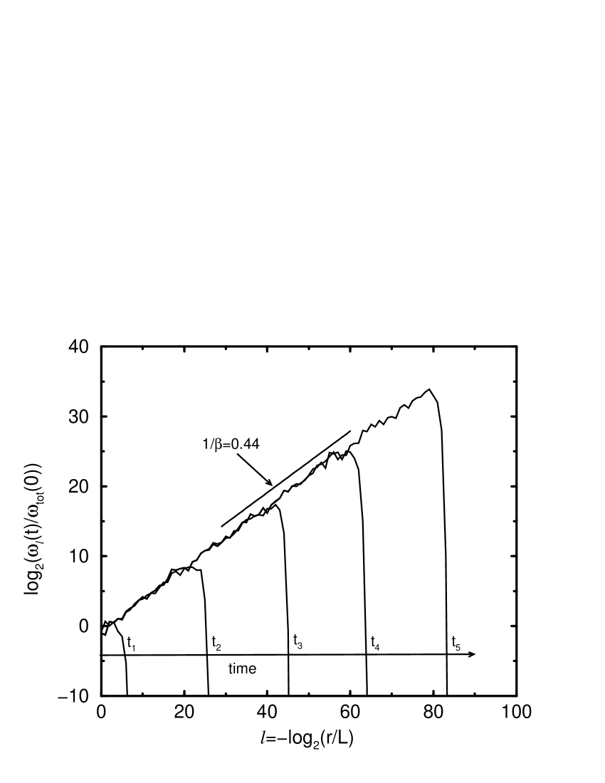
FIG. 4.: The vorticity $\omega_{\ell}$ within a shell $\ell$ as function of level number. The maximum value, which is reached at the front, diverges like $\tau^{-1}$ in time.

Since $\omega$ has units of inverse time, this maximum diverges like $\tau^{-1}$, which we confirmed numerically. This means the singularity observed in the REWA model is consistent with the criterion by Beale, Kato, and Majda [22], that the maximum of the vorticity should diverge at least as fast as $\tau^{-1}$ for a true Euler singularity. Because the exponent of the vorticity is known, we used the scaling relation

$$\max_{\ell}\{\omega_{\ell}\}\sim(t^{\ast}-t)^{-1}$$ (12)

to fit the value of the singular time $t^{\ast}$.

Next we look at the possible influence of initial conditions on the singularity. In Fig. 5

=0.5

FIG. 5.: The singularity for two different initial conditions. If the exponent is smaller than 2 initially, only the front moves. If it is 2, all scales move on the same time scale initially.

we chose the energy to have a nontrivial distribution at the initial time. For this distribution we chose two power laws, one with an exponent smaller than $\alpha$, the other larger. As seen in the figure, in both cases the solution settles on the same slope, with the same universal shape at the front. We can thus conclude that the singularity is universal except for the value of the singular time $t^{\ast}$ and the energy scale. This is of course only true apart from small fluctuations of the energy. These result from the complicated chaotic motion of Fourier modes underlying the excitation of small scales. However at the front one is very far from equilibrium, so fluctuations in the energy transfer are small compared with its absolute value.

There is another interesting observation to be made in Fig. 5, which hints to the observed universality. If the exponent of the energy distribution is $0.8$ initially, only the front of the distribution moves, the contribution from larger scales remains static. This is because $\tau_{r}=(r^{2}/E)^{1/2}=r^{1-\alpha/2}$ represents a local time scale. Hence as long as $\alpha<2$, only the smallest available scale moves, since it has the shortest time scale. The limiting case $\alpha=2$ is the other initial distribution given in Fig. 5, and indeed it now evolves on all length scales. But as soon as the newly formed front overtakes the old one, it again only grows from its front, since the slope behind it is now smaller than $2$. Hence in each case universality results from the fact that growth is determined only from the local properties of the front.

Having seen that the characteristic length and time scales of the singularity behave like power laws, we see next whether the whole sequence of profiles can be rescaled to fall onto a single master curve. To that end, we first nondimensionalize length and time. If $L$ is a length where the energy already has its scaling form, and $E_{0}$ is the energy on that scale, one can introduce the nondimensional quantities

$$\tilde{r}=r/L,\ \tilde{E}_{\ell}=E_{\ell}/E_{0},\ \tilde{t}=t(E_{0}/L^{2})^{1/2}\quad.$$ (13)

Using these, the energy is expected to scale like

$$\tilde{E}_{\ell}(\tilde{\tau})={\tilde{r}}^{\alpha}\Phi(\xi)\quad,\xi=\frac{\tilde{r}}{{\tilde{\tau}}^{\beta}}\quad,$$ (14)

where $\Phi$ is a universal function. In Fig. 6

=0.5

FIG. 6.: The scaling function of the energy $\Phi(\xi)$ determined from simulations of the REWA cascade using the rescaling (14). It is well fitted by a functional form proposed originally [2] for singularities of the full Euler equation.

the energies at different distances from the singularity are superimposed according to (14). The values of the energy at different levels is marked by crosses. Allowing for some fluctuations, the scaling relation is obeyed very well. Owing to the rescaling (13),(14), $\Phi$ asymptotes to $1$ as $\xi\rightarrow\infty$, and the collapse is the same for all initial conditions. Finally we note that $\Phi$ is fitted very well by

$$\Phi(\xi)=\exp(-5\cdot 10^{-4}/\xi)\quad,$$ (15)

which is a functional form of the energy spectrum proposed by Brachet et al. [2]. We will comment on the relation between our work and [2] in the discussion.

IV Towards an analytical description

We now develop an analytical theory for the form of the singularity which will also explain its universality, i.e. independence of initial conditions. As a basis we use a simple model for the energy transfer [16], which has been used before to describe the stationary state of developed turbulence [14]. The energy transfer is split into two parts, one deterministic, the other stochastic:

$$T_{\ell\rightarrow\ell+1}(t)=T^{(det)}_{\ell\rightarrow\ell+1}(t)+T^{(stoch)}_{\ell\rightarrow\ell+1}(t)\quad.$$ (16)

Once $T_{\ell\rightarrow\ell+1}(t)$ is specified, conservation of energy (6) results in an equation of motion for the energy. The deterministic part expresses the tendency of the cascade to establish equipartition of energy between its members. The stochastic part represents the chaotic mixing of the individual Fourier modes. If in addition we assume that both $T^{(det)}_{\ell\rightarrow\ell+1}(t)$ and $T^{(stoch)}_{\ell\rightarrow\ell+1}(t)$ only depend on the neighboring values of the energies, one ends up with the expressions [14]

$$T_{\ell\rightarrow\ell+1}^{(det)}(t) = D\frac{2^{\ell}}{L}\left(E_{\ell}^{3/2}(t)-E_{\ell+1}^{3/2}(t)\right),$$ (18)

$$T_{\ell\rightarrow\ell+1}^{(stoch)}(t) = R\left(\frac{2^{(\ell+1)}}{L}\right)^{1/2}(E_{\ell}(t)E_{\ell+1}(t))^{5/8}\xi_{\ell+1}(t)\quad.$$ (19)

The powers appearing in (16) are derived from dimensional considerations, and $\xi$ represents a Gaussian white noise with $\left<\xi_{\ell}(t)\right>=0$ and $\left<\xi_{\ell}(t)\xi_{\ell^{\prime}}(t^{\prime})\right>=2\delta_{\ell\ell^{\prime}}\delta(t-t^{\prime})$. We use Ito’s definition in equation (19). Together with (6), (16) is a Langevin equation for the motion of a cascade, so we will refer to it as the Langevin model. It has been shown that the model given by (6),(16) exhibits multifractal scaling in a stationary turbulent state, and anomalous scaling exponents can be calculated analytically [16]. At the same time it gives an excellent description of the turbulent state of the REWA cascade [14].

=0.5

FIG. 7.: The same scaling function $\Phi$ as in Figure 6, but for the Langevin model (6),(16). The crosses represent the full model, the full line corresponds to the deterministic case $R=0$.

Figure 7 shows a simulation of the model equations (6),(16) at zero viscosity, with energy concentrated in the largest scale initially. The profiles have been rescaled as in (14), which again leads to a collapse very similar to that of Fig. 6. The exponent $\alpha=1.24$ is slightly larger than that found for the REWA cascade. The values of the free parameters $D$ and $R$ in (16) are taken from [14]:

$$D=6.5\cdot 10^{-2}\quad,R=4.4\cdot 10^{-2}\quad.$$ (20)

The amplitude $D$ is of particular significance, since it determines the effectiveness of the energy transfer. If $D$ gets larger, the front reaches a given scale at an earlier time, as we are going to see in more detail below.

On the other hand, the noise strength $R$ is insignificant for the formation of the singularity, as fluctuations are small, in agreement with the result found for the REWA cascade. This is to be expected since the motion of the singularity is dictated by the front which is very steep. Thus the deterministic part (18), which consists of an energy difference will dominate the stochastic part (19). We verified this by putting $R$ to zero, leaving everything else unchanged. The result is shown as the solid line in Fig. 7, which is a perfect fit to the fluctuating data of the stochastic cascade.

Our first approximation will thus be to include only the deterministic part of the Langevin model in our analytical description. A second approximation is of a more technical nature. It is seen in Fig. 7 that the sequence of level energies form a reasonable approximation of a continuous curve. This motivates us to pass to a continuum limit, where the ratio of length scales between two levels approaches one, leading to a less cumbersome description in terms of differential equations. We introduce $\lambda$ as the ratio of length scales, which means that the length scale on level $\ell$ is $r=\lambda^{-\ell}L$. As $\lambda$ approaches 1, $E_{\ell}$ can be written as a continuous variable $E=E(r)$. Replacing $2^{-\ell}L$ by $\lambda^{-\ell}L$ in (6) and (16), and performing the limit $\lambda\rightarrow 1$, one ends up with

$$\partial_{t}E(r,t)=\bar{D}r\partial^{2}_{r}E^{3/2}(r,t),$$ (21)

where $\bar{D}=D(\ln\lambda)^{2}$ is a rescaled coupling constant. The equation of motion (21) is the one our subsequent analytical description is based on.

We now look for self-similar solutions of (21) of the form

$$\tilde{E}({\tilde{r}},\tilde{\tau})={\tilde{r}}^{\alpha}\Phi(\xi)\quad,\xi={\tilde{r}}/{\tilde{\tau}}^{\beta}\quad,$$ (22)

in direct analogy to (14). Plugging this into the equations of motion, we find that the explicit dependence on $\tilde{r}$ is eliminated by demanding that $\beta=2/(2-\alpha)$, so we recover the scaling relation (10). As a result, we are left with a similarity equation which depends on $\xi=\tilde{r}/{\tilde{\tau}}^{\beta}$ alone:

$$\frac{2}{2-\alpha}\xi^{2-\alpha/2}\Phi^{\prime}(\xi) = \frac{3}{2}\bar{D}\bigg{[}\alpha(\frac{3}{2}\alpha-1)\Phi^{3/2}(\xi)+3\alpha\xi\Phi^{1/2}(\xi)\Phi^{\prime}(\xi)+\frac{1}{2}\xi^{2}\Phi^{-1/2}(\xi)\Phi^{\prime 2}(\xi)$$ (24)

$$\hskip 56.9055pt+\xi^{2}\Phi^{1/2}(\xi)\Phi^{\prime\prime}(\xi)\bigg{]}\quad.$$

In the following section we will show that (24) possesses a unique physical solution, which fixes both the similarity function $\Phi$ and the exponent $\alpha$.

V Selection

Since (24) is of second order, one needs two initial conditions to uniquely fix the solution. As noted earlier, $\Phi$ asymptotes to a constant at infinity. Since scales have been normalized according to (13), this constant is one, leaving us with the boundary conditions

$$\left.\begin{array}[]{lcl}\Phi(\xi)&\rightarrow&1\\ \Phi^{\prime}(\xi)&\rightarrow&0\\ \end{array}\right\}\xi\rightarrow\infty\quad.$$ (25)

The coupling strength $\bar{D}$ can be eliminated by the transformation

$$\zeta=\bar{D}^{2/(\alpha-2)}\xi\quad.$$ (26)

This means that for large coupling strengths the position of the front moves towards larger $\xi$. Thus a given length scale is reached earlier, as to be expected on physical grounds. For our discussion of universal solutions we will consider the equation in the independent variable $\zeta$, where $\bar{D}$ has been eliminated.

To find explicit solutions, we expand the similarity equation around $\zeta=\infty$. Using the boundary conditions, this leads to an asymptotic expansion

$$\Phi(\zeta)=\sum_{i=0}^{\infty}b_{i}\zeta^{-i/\beta}\quad,\quad b_{0}=1\quad,$$ (27)

where the coefficients $b_{i}$ depend on $\alpha$ alone. Given a sufficiently large $\zeta_{init}$, (27) can be used to generate an initial condition at $\zeta_{init}$. This initial condition then allows to integrate the similarity equation numerically towards small $\zeta$. Hence there is a unique solution for each $\alpha$, while we expect the partial differential equation (21) to select a unique $\alpha$. To understand this, we now look at the behavior of solutions for different $\alpha$. Three cases arise, which are shown in Fig. 8.

=0.5

FIG. 8.: Solutions of the similarity equation (24) for three different $\alpha$. For $\alpha$ greater than a critical value $\alpha_{c}=1.12045$, the tip of the front becomes fractal. The inset shows a blow-up of this behavior on a logarithmic scale.

If $\alpha$ is smaller than a critical value $\alpha_{c}=1.12045\pm 10^{-5}$ the profile ends in a sharp front, similar to the front observed in simulations both of the REWA and the Langevin cascade. The profile is zero below a front position $\zeta_{0}$, for $\zeta>\zeta_{0}$ $\Phi$ behaves asymptotically like $\Phi\sim(\zeta-\zeta_{0})^{2/3}$. This corresponds to a local expansion of the form

$$\Phi(\zeta)=\sum_{i=0}^{\infty}a_{i}(\zeta-\zeta_{0})^{(2+i)/3}\quad.$$ (28)

If on the other hand $\alpha$ is larger than $\alpha_{c}$, the front becomes unstable and levels off to form a flat plateau. As shown in more detail in the appendix (see also the inset in Fig. 8), this plateau dips down again at a smaller value of $\zeta$, only to form another plateau as the second front becomes unstable. This process repeats itself, to form a fractal tip which asymptotes to zero. Clearly this is not an acceptable solution, at the very least because it would correspond to energy being transported instantly across all levels.

This indicates that there is something special about solutions at $\alpha=\alpha_{c}$, which separates the region of sharp and fractal fronts. Indeed, a more careful analysis, which is detailed in the appendix, reveals that at the critical $\alpha$ the asymptotics at the front position is now

$$\Phi(\zeta)=\sum_{i=0}^{\infty}\bar{a}_{i}(\zeta-\zeta_{0})^{2+i}\quad.$$ (29)

But although this amounts only to a slight difference in the appearance of the fronts in Fig. 8, the solution at $\alpha_{c}$ is the one which is selected. This comes from an argument similar to that advanced for front propagation into an unstable medium [28]. Indeed, on a logarithmic scale, i.e. by level number, the self-similar solution (22) corresponds to a front propagating at a constant speed $\alpha$. In our problem, the situation is actually reverse to that of [28]: of all possible solutions, the one with the highest speed will eventually take over, while the slow solutions are left behind. On the time scale set by the front, they no longer move, and thus drop out of the problem. This explains the universality observed earlier: independent of initial conditions, only one front with a given exponent $\alpha$ is observed. We also checked the validity of our selection argument directly, by simulating the Langevin cascade (6), (16) with $R=0$ for smaller and smaller scaling factors $\lambda$. Extrapolating to $\lambda=1$, we were able to confirm the value of $\alpha_{c}$ to five decimal places.

In Table I we summarize some of the values of the exponent $\alpha$ obtained for different cascades. The REWA cascade with $26$ modes, which we considered throughout this paper, is called “small cascade” here, to distinguish it from another mode selection with $74$ modes. The Langevin cascade with the same scale factor $\lambda=2$ as the REWA cascades gives a somewhat larger value.

	$\alpha$
small cascade, N=26	$1.12\pm 0.01$
large cascade, N=74	$1.17\pm 0.01$
Langevin cascade, $\lambda=2$	$1.24\pm 0.01$
similarity equation	$1.12045\pm 10^{-5}$

TABLE I.: Compilation of different values of the exponent of the shell energies $\alpha$. The first two values are from simulations of the REWA cascade with two different wave vector sets. The third line refers to the model equations (6),(16), the last line is the result of our similarity theory.

However, the overall variation of the exponent $\alpha$ is only in the order of 10%. This strongly supports the claim that our analytical theory has captured the physical mechanism behind the selection of a singular front for all the models considered.

Another important quantity is the position of the front, which for the similarity solution is found to be

$${\tilde{r}}_{c}=\bar{D}^{2/(2-\alpha)}\zeta_{0}{\tilde{\tau}}^{\beta}.$$ (30)

Once again we see that for large $\bar{D}$ a given length is excited at earlier times. The coupling $\bar{D}$ is the only parameter to be determined for a comparison between theory and simulation of the REWA cascade. We adjusted $\bar{D}$ such that the average energy in a turbulent state agrees with the value determined for the REWA cascade [14]. Thus we are able to predict $\Phi$ without adjustable parameters. The comparison between the solution of the similarity equation at $\alpha=\alpha_{c}$ and the numerical simulation of the REWA cascade is shown in Fig. 9.

=0.5

FIG. 9.: Comparison between the similarity theory and and the numerical simulation of the REWA cascade. The free parameter $\bar{D}$ of the similarity equation has been determined from an independent measurement of the turbulent state.

The agreement is quite good, although there is some difference in the shape of the front. It makes sense that for this shape, which describes the excitation of Fourier modes, the detailed coupling structure of modes matters to some degree. This shows that the formation of a singularity in a very complicated system of coupled Fourier modes is indeed described by a very simple physical principle: the tendency of the cascade to establish equipartition of energy.

VI Discussion

Roughly speaking, two different methods have been used to numerically treat the formation of singularities in the Euler equation. One relies on a Fourier representation of the velocity field [2, 9], the other tries to track the vorticity in real space [3, 5]. Given a simulation with perfect resolution, the results should be the same, but in effect there are two different physical pictures underlying the two approaches. A spectral approach is preferable if a singularity generically results from the interaction of Fourier modes, as suggested originally by Onsager [1]. A spatial picture would show a uniformly (multi)-fractal structure.

Vorticity dynamics, on the other hand, would be more useful if a singularity results from a specific spatial structure, like the meeting of two antiparallel vortex tubes [3]. Other, more complicated structures have been proposed in two-dimensional, axisymmetric flow [5, 6].

Since the spatial resolution of the REWA cascades studied here is quite low, it is hard to speculate about the physics of vortex tubes. We must rely on the spectral picture being relevant, which was analyzed in detail by Brachet et al. [2]. They find that the large wavenumber part of the energy spectrum is well described by

$$E(k,t)=ak^{-n(t)}e^{-2\delta(t)k}\quad.$$ (31)

This is very similar to the form of the energy distribution observed for our case. However, an important difference is that (31) predicts excitation of all scales, while in the REWA model the energy drops to zero. This difference, which becomes noticeable for energies smaller than those shown in Fig. 6, comes from the absence of non-local interactions in the REWA model, which would excite small scales instantly. Since the energy $E_{\ell}$ of a shell represents the energy spectrum integrated over an octave in wavenumber, $n(t)$ is to be identified with the exponent $\alpha+1$. If in addition $\delta(t)$ was chosen to behave like $\tau^{\beta}$, one would end up with our scaling form (22).

However, although $n(t)$ converges to a value close to $4$ [2], this is much larger than the value $\alpha+1=2.12$ we find. Other workers [8] find $n$ close to $3$ asymptotically. This is closer to our value, but still at the boundary where the largest scales would move fastest, according to our estimate $\tau_{r}=r^{1-\alpha/2}$. Our simulations are self-consistent since for $\alpha\geq 2$ nonlocal interactions would become dominant [1, 23, 24], which have not been included in our description. It would of course be of great importance to investigate whether local or non-local interactions are dominant for the full Euler equation.

A second significant difference between the results of [2] and our work is that $\delta(t)$ does not go to zero in finite time, but rather behaves like

$$\delta(t)=\delta_{0}e^{-t/T}\quad.$$ (32)

This corresponds to a singularity only in infinite time. All results of [2] were later confirmed in [9] using greater resolution and more general initial conditions. But of course there is also a good possibility that if greater resolution allows to continue the simulation still further, a crossover from (32) to a finite time singularity is seen.

A definite answer whether singularities of the three-dimensional Euler equation exist can only be given by considering the full equations. Nevertheless, our study shows that structures exist in inviscid flow which show blow-up in finite time. They are consistent with the divergence of the vorticity like $\tau^{-1}$, and the existence of a local cascade. The scaling structure of the singularity found here can thus serve as a guideline for further studies of the full equations. The more general structures possible in the fully resolved flow can of course be more singular than ours, so we expect the structures appearing in our mode-reduced systems to be dominated by even more singular contributions. Conversely, there is also the possibility that the modes not taken into account in our study will interact with the reduced mode system to keep it from becoming singular. One possible way to study this would be to selectively take non-local interactions into account, to find out what modifications they imply for our analysis.

A particularly intriguing aspect of the present work is the novel way the scaling exponent is selected as the “speed” of a marginally stable solution. This adds another variety to the existing mechanisms which determine the scaling exponents of singularities which are not determined from dimensional arguments. Other selection mechanisms for this scaling behavior of the second kind (in Barenblatt’s [25] terminology) are found in [26] and in [27].

Formally, the selection mechanism is quite similar to that of marginally stable solutions of equations of the form [28]

$$\partial_{t}\phi=\partial^{2}_{x}\phi+F(\phi)\quad.$$ (33)

However, solutions to this equation do not drop to zero at a finite value of $x$ but rather decay exponentially away from the front. For this reason we are not able to repeat the linear stability analysis presented for example in [28], since the front of our solution is very steep. In that respect it is more similar to solutions of the porous medium equation [29], which in one dimension reads

$$\partial_{t}u=\partial^{2}_{x}u^{m}\quad.$$ (34)

Solutions to this equation form a front which drops to zero, like ours. However, although for $m=3/2$ (34) looks quite similar to (21), the factor $r$ in (21) represents a very serious complication. This is because its value at the front goes to zero at the singularity, giving a very singular diffusion constant. Thus again we are not able to carry over the mathematically rigorous results known for the porous medium equation. Still we believe that the combination of numerical evidence and analysis of the similarity equation conclusively demonstrates that the marginal solution is indeed the one selected for our equation (21). This adds to the generality of the marginal stability concept.

Finally, we would like to stress the fact that the cascades studied in this paper give a coherent picture of both Euler singularities and fully developed turbulence. In fact the same is true for a scalar shell model recently studied by Dombre and Gilson [30]. They also found unique singular solutions of the inviscid equations, but whose spectrum is less steep than Kolmogorov’s. In addition, they propose a connection between inviscid singularities and intermittent fluctuations. We started to explore this connection in the second section, but this has to be pursued further. We suspect the situation will be quite different from that of the scalar shell model, because our singular spectrum is steeper than that of a stationary cascade. In particular, it would be interesting to study the interaction between the most singular solutions and viscosity, leading to a turbulent state. Since the most singular solution with $\alpha=\alpha_{c}$ is regularized by viscosity, other solutions with $\alpha<\alpha_{c}$ will become relevant as well. So it may be the whole spectrum of singular solutions which is relevant to the turbulent state.

Similarity solutions

Here we discuss the transition of solutions of the similarity equation (24) from regular to fractal tips in more detail. The similarity variable is rescaled according to $\zeta=\bar{D}^{2/\alpha-2}\xi$.

The invariance of (24) under scale transformations $\zeta\to\mu\zeta$, $\Phi\to\mu^{2-\alpha}\Phi$ can be used to transform it to a first order equation

$$v^{\prime}(u)=\frac{1}{u^{1/2}v(u)}\left[\frac{4}{3}u+\frac{4}{6-3\alpha}v(u)-4u^{3/2}-5u^{1/2}v(u)-\frac{1}{2}u^{-1/2}v^{2}(u)\right]$$ (35)

with

$$u(\zeta)=\zeta^{\alpha-2}\Phi(\zeta)$$ (36)

$$v(u)=\zeta u^{\prime}(\zeta)\quad.$$ (37)

Primes always refer to derivatives with respect to the argument. It follows from (36) that $u$ goes to zero both for $\zeta$ going to infinity and $\Phi$ going to zero. Thus all solutions start out at $u=0$, corresponding to $\zeta=\infty$, shown by the full line in Fig. 10. To form a regular tip, they must return to $u=0$ (dashed and dot-dashed lines), which is the case for $\alpha\leq\alpha_{c}$. For $\alpha>\alpha_{c}$, on the other hand, $v(u)$ enters a limit cycle, which corresponds to the fractal tip (dotted line).

=0.5

FIG. 10.: Solutions of the first-order version of the similarity equation. The three different types of solutions correspond directly to Fig. 8. The fractal tip, observed for $\alpha>\alpha_{c}$ corresponds to a limit cycle.

Equation (35) becomes singular for $u=0$ or $v=0$, thus only local solutions exist either in the domain $0<u<u_{max}$ or $u_{min}<u<u_{max}$ with $v(u_{max/min})=0$. To form a complete solution, local solutions have to be matched at the points indicated in Fig. 10.

Three different expansions exist around the point $u=0$:

$$v(u)=u^{\gamma}\sum_{i=0}^{\infty}c_{i}^{(\gamma)}u^{i/2}$$ (38)

$$\gamma=1,-\frac{1}{2},\frac{1}{2}\quad,$$ (39)

which corresponds directly to the three expansions (27), (28), and (29) of $\Phi$. The coefficients $c_{i}^{(1)}$, which describe the behavior of $\Phi$ at infinity, are determined recursively from

$$c_{0}^{(1)}=\alpha-2\quad,$$ (40)

$$c_{i}^{(1)}=\frac{3(2-\alpha)}{4}\left(4\delta_{i1}+5c_{i-1}^{(1)}+\sum_{j=0}^{i-1}\left(\frac{3}{2}+\frac{j}{2}\right)c_{j}^{(1)}c_{i-j-1}^{(1)}\right)\quad.$$ (41)

The case $\gamma=1/2$, which corresponds to a tip of the form $\Phi(\zeta)=\zeta_{0}^{-\alpha}(c_{0}^{(1/2)})^{2}(\zeta-\zeta_{0})^{2}/4$ is determined by

$$c_{0}^{(1/2)}=\frac{4}{3(2-\alpha)}$$ (42)

$$c_{i}^{(1/2)}=\frac{-2\delta_{i1}+6\delta_{i2}+15c_{i-1}^{(1/2)}/2+\sum_{j=1}^{i-1}\left(3/2+3j/4\right)c_{j}^{(1/2)}c_{i-j}^{(1/2)}}{2/(2-\alpha)-3\left(1+i/4\right)c_{0}^{(1/2)}}\quad.$$ (43)

This is the critical case. On the other hand, solutions with $\alpha<\alpha_{c}$ have a tip $\Phi(\zeta)=\zeta_{0}^{1-\alpha}(3c_{0}^{(-1/2)}/2)^{(2/3)}(\zeta-\zeta_{0})^{2/3}$. In that case the constant $c_{0}^{(-1/2)}$ is open and the higher order coefficients are calculated from

$$c_{i}^{(-1/2)}=\frac{4}{3ic_{0}^{(-1/2)}}\left(2\delta_{i5}-6\delta_{i6}+\frac{2}{2-\alpha}c_{i-2}^{(-1/2)}-15c_{i-3}^{(-1/2)}/2-\sum_{j=2}^{i-2}(3j/4)c_{j}^{(-1/2)}c_{i-j}^{(-1/2)}\right)\quad.$$ (44)

All expansions (40)-(44) are asymptotic in nature, but are extremely good everywhere except in a small neighborhood of $u_{max}$. To do the matching at $u_{max}$, equation (35) has to be integrated numerically.

The local behavior at $u_{max}$ is

$$v(u)=C\left(u_{max}-u\right)^{1/2}\mbox{ with }C=\pm\left(8(u_{max}-\frac{1}{3}u_{max}^{1/2})\right)^{1/2}\quad,$$ (45)

where the solid line of Fig. 10 corresponds to negative $C$, the other branches to positive $C$. At a given $\alpha$, for each of the three branches $\gamma=1,-1/2$, and $1/2$ one can extrapolate to the asymptotic behavior (45) to determine $u_{max}$. A matching of the branch $\gamma=1$ on the branch $\gamma=1/2$ is only possible for one $\alpha$, which is the critical $\alpha=\alpha_{c}=1.12045$. For $\gamma=-1/2$ the free parameter $c_{0}^{(-1/2)}$ can be used to match $u_{max}$, and this turns out to be possible only for $\alpha<\alpha_{c}$.

If $\alpha>\alpha_{c}$, there is no branch which returns to $u=0$, and the solution has to be continued numerically through the matching point. The resulting branch goes to $v=0$ at a finite $u=u_{min}$, where it can be matched onto the original solution with $\gamma=1$. This means the solution ends up on a limit cycle. From the definition of $u$ (cf. (36)) it is clear that the sequence of tips of $\Phi(\zeta)$ approximates a power law $\Phi\sim\zeta^{2-\alpha}$, as shown in the inset of Fig. 8.

REFERENCES

- [1] L. Onsager, “Statistical hydrodynamics”, Nuovo Cimento 6, 279 (1949)
- [2] M.E. Brachet et al., “Small-scale structure of the Taylor-Green vortex”, J. Fluid Mech. 130, 411 (1983)
- [3] E. D. Siggia, “Collapse and amplification of a vortex filament”, Phys. Fluids 28, 794 (1985)
- [4] A. Pumir and E. D. Siggia, “Collapsing solutions of the 3-D Euler equations”, Phys. Fluids A 2, 220 (1990)
- [5] R. Grauer and T. C. Sideris, “Numerical Computation of 3D Incompressible Ideal Fluids with Swirl”, Phys. Rev. Lett. 67, 3511 (1991)
- [6] A. Pumir and E. D. Siggia, “Development of singular solutions of the axisymmetric Euler equation”, Phys. Fluids A 4, 1472 (1992)
- [7] M. J. Shelley, D. I. Meiron, and S. A. Orszag, “Dynamical aspects of vortex reconnection of perturbed anti-parallel vortex tubes”, J. Fluid Mech. 246, 613 (1993)
- [8] R. M. Kerr, “Evidence for a singularity of the three-dimensional, incompressible Euler equations”, Phys. Fluids A 5, 1725 (1993)
- [9] M.E. Brachet et al., “Numerical evidence of smooth self-similar dynamics and possibility of subsequent collapse for three-dimensional ideal flows”, Phys. Fluids A 4, 2845 (1992)
- [10] J. Eggers, “Universal pinching of 3D Axisymmetric Free-Surface Flow”, Phys. Rev. Lett. 71, 3458 (1993)
- [11] A. N. Kolmogorov, “The local structure of turbulence in incompressible viscous liquids”, Dokl. Akad. Nauk SSSR 30, 9 (1941)
- [12] J. Eggers and S. Grossmann, “Does deterministic chaos imply intermittency in fully developed turbulence?”, Phys. Fluids A 3, 1985 (1991)
- [13] S. Grossmann and D. Lohse, “Scale resolved intermittency in turbulence”, Phys. Fluids 6, 611 (1994)
- [14] C. Uhlig and J. Eggers, “Local coupling of shell models leads to anomalous scaling”, Z. Phys. B to be published (1996)
- [15] M. Nelkin, “What do we know about self-similarity in fluid turbulence?”, J. Stat. Phys. 54, 1 (1989).
- [16] J. Eggers, “Multifractal scaling from nonlinear turbulence dynamics: analytical methods”, Phys. Rev. E 50, 285 (1994)
- [17] A. M. Obukhov, “Some general properties of equations describing the dynamics of the atmosphere”, Atmos. Ocean. Phys. 7, 471 (1971).
- [18] E. B. Gledzer, “Systems of hydrodynamic type admitting two quadratic integrals of motion”, Sov. Phys. Dokl. 18, 216 (1973).
- [19] M. Yamada and K. Ohkitami, “Lyapunov spectrum of a chaotic model of three-dimensional turbulence”, J. Phys. Soc. Jpn 56, 4210 (1987).
- [20] M. H. Jensen, G. Paladin, and A. Vulpiani, “Intermittency in a cascade model for three-dimensional turbulence”, Phys. Rev. A 43, 798 (1991).
- [21] U. Frisch, “Turbulence”, (Cambridge University Press, 1st ed., 1995)
- [22] J.T. Beale, T. Kato, and A. Majda, “Remarks on the breakdown of smooth solutions for the 3D Euler equations”, Comm. Math. Phys. 94, 61 (1984)
- [23] G. L. Eyink, “Energy dissipation without viscosity in ideal hydrodynamics, I”, Physica D 78, 222 (1994)
- [24] G. L. Eyink, “Local energy flux and the refined similarity hypothesis”, J. Stat. Phys. 78, 335 (1995)
- [25] Barenblatt, G. I., Scaling, self-similarity, and intermediate asymptotics, (Cambridge University Press, 1996)
- [26] A. Guderley, “Starke kugelige und zylindrische Verdichtungsstösse in der Nähe des Kugelmittelpunktes bzw. der Zylinderachse”, Luftfahrtforschung 19, 302 (1942)
- [27] D. T. Papageorgiou, “On the breakup of viscous liquid threads”, Phys. Fluids 7, 1529 (1995)
- [28] W. van Saarloos, “Front propagation into unstable states: Marginal stability as a dynamical mechanism for velocity selection”, Phys. Rev. A 37, 211 (1988)
- [29] D. G. Aronson, “The porous medium equation”, in : Nonlinear Diffusion Problems, edited by A. Fasano and M.Primicario, Lecture Notes in Mathematics, (Springer, 1986)
- [30] T. Dombre and J.-L. Gilson, “Intermittency, chaos and singular fluctuations in the mixed Obukhov-Novikov shell model of turbulence”, preprint, October 1995