Abstract

The exact and semiclassical quantum mechanics of the elliptic billiard is investigated. The classical system is integrable and exhibits a separatrix, dividing the phase space into regions of oscillatory and rotational motion. The classical separability carries over to quantum mechanics, and the Schrödinger equation is shown to be equivalent to the spheroidal wave equation. The quantum eigenvalues show a clear pattern when transformed into the classical action space. The implication of the separatrix on the wave functions is illustrated. A uniform WKB quantization taking into account complex orbits is shown to be adequate for the semiclassical quantization in the presence of a separatrix. The pattern of states in classical action space is nicely explained by this quantization procedure. We extract an effective Maslov phase varying smoothly on the energy surface, which is used to modify the Berry-Tabor trace formula, resulting in a summation over non-periodic orbits. This modified trace formula produces the correct number of states, even close to the separatrix. The Fourier transform of the density of states is explained in terms of classical orbits, and the amplitude and form of the different kinds of peaks is analytically calculated.

1 Introduction

The semiclassical quantization of a Hamiltonian system is deeply connected to the structure of its phase space. The generic Hamiltonian system contains a complicated mixture of near-integrable and chaotic motion, and a consistent semiclassical quantization scheme does not exist for the generic case. It does exist, however, in the non-generic limiting cases, the integrable and the ergodic systems.

During the last two decades much progress has been made for ergodic systems. The Gutzwiller trace formula gives the density of states as a sum over periodic orbits [1, 2, 3]. It works well if all periodic orbits are unstable and isolated, i.e. for hyperbolic systems, and is the starting point for most calculations in this field.

The investigation of integrable systems reaches back to the beginning of quantum mechanics. Bohr and Sommerfeld, among others, succeeded in the quantization of actions. The hydrogen atom is the most famous example. The deficiency of the old quantum mechanics to calculate, e.g., the spectrum of the helium atom was set into clear light by Einstein [4]. He formulated the Bohr-Sommerfeld quantization conditions in terms of invariant tori which foliate the phase space of integrable systems. Moreover he noted that this foliation is absent in generic systems, such that this quantization scheme fails. The same year when Schrödinger introduced his famous equation Brillouin explained that the quantization of tori is a consequence of the single-valuedness of the quantum mechanical wave functions. Keller showed how the quantization conditions have to be modified because of caustics in the classical motion [5]. For an integrable system with $f$ degrees of freedom described by its phase space variables $({\bf q,p})=(q_{1},...,q_{f},p_{1},...,p_{f})$ the Einstein-Brillouin-Keller (EBK) quantization conditions for the actions $I_{i}$ read

$$I_{i}=\frac{1}{2\pi}\oint_{\gamma_{i}}{\bf p}\,d{\bf q}=\hbar(n_{i}+\frac{\alpha_{i}}{4})\,,$$ (1)

where the integration is to be taken along $f$ topologically independent paths $\gamma_{i}$ around the $f$-torus, and $\alpha_{i}$ are the Maslov indices due to the classical caustics.

This paper deals with a nontrivial example of an integrable system: the planar elliptic billiard. Classically “billiard” refers to a system in which a point particle moves freely inside a domain and is elastically reflected at the domain boundary. The corresponding quantum mechanical problem is to solve the Laplace equation inside the domain with Dirichlet boundary condition. Billiards have become popular because for them on the one hand the classical calculations are easier than for systems with smooth potential, and on the other hand they allow for experimental measurements, e.g.  [6, 7, 8]. Jacobi [9] showed that elliptic coordinates separate the geodesic flow on the ellipsoid, which contains our billiard as a limiting case. The same coordinate system leads to the separation of Schrödinger’s equation, including the Dirichlet boundary condition, into two Mathieu equations.

Integrability allows for a semiclassical quantization à la EBK. In our case, however, there are problems due to the presence of a separatrix. For all energies it divides phase space into regions of rotational and oscillatory motion [10]. The Maslov indices are different for the two classical regions, resulting in a discontinuity in the EBK quantization condition which in turn leads to ambiguities for states close to the separatrix. To overcome this problem it is necessary to introduce a uniform quantization condition. This can be done by investigating the asymptotics of the solutions of Schrödinger’s equation close to the separatrix, which was carried out for the elliptic billiard in [11]. We will follow a different approach based on connection matrices between the amplitudes of WKB wave functions, see [12, 13], the review of Berry and Mount [14], and the references therein. This approach can be interpreted in terms of orbits with complex classical action. A transformation of the quantum mechanical eigenvalues to classical action space allows for a unique mapping of the eigenvalues to the quantum numbers.

The discontinuity in the EBK quantization condition carries over to the Berry-Tabor trace formula [15] - the analogue of the Gutzwiller trace formula for integrable systems. The resonant tori, foliated by families of periodic orbits, take over the role of the isolated periodic orbits as the objects to be summed over. The uniformization employed in [15] incorporates the influence of orbits with negative classical action in the vicinity of isolated stable periodic orbits. We will introduce a modification of the Berry-Tabor trace formula which takes care of the separatrix in terms of an effective Maslov phase varying smoothly across. It will turn out that in order to correctly produce eigenstates close to the separatrix the summation has to be taken over non-periodic orbits, i.e. over classical tori with in general irrational winding number. This trace formula incorporates all kinds of classically non-real orbits.

The Berry-Tabor trace formula was further investigated by Richens [16], who showed that it contains contributions of the stable isolated periodic orbits, whose contributions are equal to the corresponding terms in the Gutzwiller’s trace formula [3]. We will use his results in the study of the length spectrum, extending the “inverse quantum chaology”, see e.g. [17, 18], to integrable systems.

After completion of this work there independently appeared a preprint by M. Sieber [19], whose first part contains considerations similar to parts of our paper. Nevertheless, the key point of his paper being the semiclassical consequences of the deformation of an elliptic billiard to an oval, while we concentrate on the separatrix and on complex orbits, the overlap is only mild.

The organization of our paper is as follows. We start with a short summary of the classical facts in sec. 2 and perform the exact quantum mechanical calculations in sec. 3. In sec. 4 we introduce a uniform WKB quantization condition. This method gives an effective Maslov phase which is used to modify the Berry-Tabor trace formula for systems with a separatrix in sec. 5, resulting in a sum over non-periodic orbits. The appearance of resonant tori in the length spectrum, i.e. in the Fourier transform of the density of states, is investigated in sec. 6. The conclusion and an outlook are given in sec. 7.

2 Classical mechanics

The classical dynamics of the planar elliptic billiard has been investigated by many authors, e.g. [20, 10, 21, 22] and the references therein. We just give a summary of the facts important for our purpose. Scaling the longer semimajor axis to one, the boundary of the billiard is described by

$$x^{2}+\frac{y^{2}}{1-a^{2}}=1,\qquad 0\leq a<1\ ,$$ (2)

with foci at $(x,y)=(\pm a,0)$. The boundary of the ellipse is a $\phi$-coordinate line of the elliptic coordinates $(\rho,\phi)$ given by

$$\begin{array}[]{r}(x,y)=\left(\displaystyle a\cos{\phi}\cosh{\rho},a\sin{\phi}\sinh{\rho}\right)\ ,\end{array}$$ (3)

where the coordinate ranges are

$$0\leq\rho\leq\rho_{\text{max}}={\text{arccosh}}(1/a),\quad 0\leq\phi\leq 2\pi\ .$$ (4)

The lines $\rho=\text{const}$ are confocal ellipses and the lines $\phi=\text{const}$ are confocal hyperbolas. Introducing the conjugate momenta $(p_{\rho},p_{\phi})$, a reflection at the boundary $\rho=\rho_{\text{max}}$ is simply described by $(\rho,\phi,p_{\rho},p_{\phi})\rightarrow(\rho,\phi,-p_{\rho},p_{\phi})$. The Hamiltonian of a freely moving particle of unit mass reads in these coordinates

$$H=\frac{p_{\rho}^{\ 2}+p_{\phi}^{\ 2}}{2a^{2}(\cosh^{2}\rho-\cos^{2}\phi)}\ .$$ (5)

Multiplying Eq. (5) with the denominator of the right hand side yields the separation constant $K$:

$$p_{\rho}^{\ 2}+(K-2Ea^{2}\cosh^{2}\rho) = 0,$$ (6)

$$p_{\phi}^{\ 2}-(K-2Ea^{2}\cos^{2}\phi) = 0\,.$$ (7)

Figure 1: Effective potentials $V_{\text{eff}}(\rho)$ and $V_{\text{eff}}(\phi)$ and the tori of the elliptic billiard. Real tori are marked by $R$ (rotations) or $O$ (oscillations). The classically forbidden motion are $TR$ (tunneling from region 1 to 2 in the radial direction), $TO$ (tunneling from region 1 to 2 in the angular direction), and $O_{c}$ and $TO_{c}$, the complex continuations of $O$ and $TO$ below the minimum of $V_{\text{eff}}(\phi)$. Orbits with complex position are indicated by a circled cross. The reason for taking negative values of $\rho$ into account will become clear in sec. 4.

Here $E>0$ is the energy, and $\kappa^{2}=K/(2E)$ is the second constant of the motion. Since $H$ and $K$ are in involution, the system is integrable and therefore the energy surface is foliated by invariant Liouville 2-tori. Each of the equations (6) and (7) can be interpreted as a Hamiltonian system with one degree of freedom, with effective energy $E_{\rho}=-E\kappa^{2}$ and $E_{\phi}=E\kappa^{2}$ respectively, and a sum of kinetic term and effective potential $V_{\text{eff}}(\rho)=-Ea^{2}\cosh^{2}(\rho)$ or $V_{\text{eff}}(\phi)=Ea^{2}\cos^{2}(\phi)$. The topologically different types of motions can be discussed in terms of the effective potentials shown in Fig. 1. It is obvious that there are only two types of classically allowed motion. For $\kappa^{2}>a^{2}$ the trajectories avoid the interior of the ellipse $\cosh(\rho)=\kappa/a$, touching its boundary between every two consecutive reflections at the billiard boundary $\rho=\rho_{\text{max}}$. This “type $R$” motion is similar to the rotational motion in a planar circular billiard. For $\kappa^{2}<a^{2}$ the trajectories always cross the $x$-axis between the foci; they are confined to the domain enclosed by the hyperbolas $\cos\phi=\pm\kappa/a$. This “type $O$” motion involves an oscillation in $\phi$. The special values $\kappa^{2}=0$ and $\kappa^{2}=1$ represent the stable oscillation along the $y$-axis ($o_{s}$) and the sliding motion along the boundary ($o_{b}$), respectively. $\kappa^{2}=a^{2}$ characterizes the separatrix motion and the unstable isolated periodic orbit. An orbit on the separatrix alternately passes through one or the other focus between reflections. The unstable periodic orbit in the center of the separatrix performs an oscillation along the $x$-axis ($o_{u}$). It is the only orbit which passes through both foci between consecutive reflections. The length of this orbit is $L_{u}=4$, the stable orbit has $L_{s}=4\sqrt{1-a^{2}}$ and the length of the sliding orbit is just the circumference $L_{b}=4{\cal E}(a)$ of the billiard. ${\cal E}(k)$ is the complete elliptic integral of the second kind in the notation of [23, 24]. The action $S$ and the period $T$ of these orbits can easily be obtained from $S=\sqrt{2E}L$ and $T=\partial S/\partial E=S/(2E)=L/\sqrt{2E}$.

The calculation of the action variables ${\mbox{\boldmath$I$\unboldmath}}=(I_{\rho},I_{\phi})=(\frac{1}{2\pi}\oint p_{\rho}d\rho,\frac{1}{2\pi}\oint p_{\phi}d\phi)$, the frequencies ${\mbox{\boldmath$\omega$\unboldmath}}=\partial H/\partial{\mbox{\boldmath$I$\unboldmath}}$, and the winding number $w=\omega_{\phi}/\omega_{\rho}$ of the elliptic billiard can be found in [10]. Since the system is invariant under reflections about the $x$- and $y$-axis, we will also consider the desymmetrized elliptic billiard, that is a quarter of the full ellipse. For type $R$ $(\kappa^{2}>a^{2})$ the actions $\tilde{I}$ and the winding number $\tilde{w}=\tilde{\omega}_{\phi}/\tilde{\omega}_{\rho}$ of the desymmetrized billiard are

$$\begin{array}[]{lllrl}\tilde{I}_{\rho}&=&\frac{\sqrt{2E}}{\pi}\;\left(\sin\chi-\kappa\;{\cal E}(\chi,\frac{a}{\kappa})\right)&=&I_{\rho}\ ,\\ \tilde{I}_{\phi}&=&\frac{\sqrt{2E}}{\pi}\kappa\;{\cal E}(\frac{a}{\kappa})&=&\pm\frac{1}{2}I_{\phi}\ ,\\ \tilde{w}&=&{\cal F}(\chi,\frac{a}{\kappa})/{\cal K}(\frac{a}{\kappa})&=&\pm 2w\ ,\end{array}$$

with $\sin^{2}\chi=\displaystyle(1-\kappa^{2})/(1-a^{2})$. For type $O$ $(\kappa^{2}<a^{2})$ they are given by

$$\begin{array}[]{lllrl}\tilde{I}_{\rho}&=&\frac{\sqrt{2E}}{\pi}\;\left(\sin\psi+\frac{a^{2}-\kappa^{2}}{a}\;{\cal F}(\psi,\frac{\kappa}{a})-a\;{\cal E}(\psi,\frac{\kappa}{a})\right)&=&\frac{1}{2}I_{\rho}\ ,\\ \tilde{I}_{\phi}&=&\frac{\sqrt{2E}}{\pi}\;\left(a\;{\cal E}(\frac{\kappa}{a})-\frac{a^{2}-\kappa^{2}}{a}\;{\cal K}(\frac{\kappa}{a})\right)&=&\frac{1}{2}I_{\phi}\ ,\\ \tilde{w}&=&{\cal F}(\psi,\frac{\kappa}{a})/{\cal K}(\frac{\kappa}{a})&=&w\ ,\end{array}$$

with $\sin^{2}\psi=\displaystyle(1-a^{2})/(1-\kappa^{2})$. ${\cal K}(k)$ is the complete elliptic integral of the first kind, ${\cal F}(\mu,k)$ and ${\cal E}(\mu,k)$ are incomplete elliptic integrals of first and second kind.

Figure 2: Energy surfaces (a) for the values $E=0.5,1,1.5,2,2.5,3$ and the winding number (b) of the desymmetrized elliptic billiard with parameter $a=0.7$. The line $\kappa^{2}=a^{2}$ ($\tilde{I}_{\rho}=\frac{1-a}{a}\tilde{I}_{\phi}$) represents the separatrix motion and the unstable oscillation along the $x$-axis. The line $\kappa^{2}=0$ ($\tilde{I}_{\phi}=0$) marks the stable oscillation along the $y$-axis, and $\kappa^{2}=1$ ($\tilde{I}_{\rho}=0$) corresponds to the sliding motion along the billiard boundary. The dotted lines represent the real complex tori of type $O_{c}$.

Figure 2a shows the energy surfaces $H({\mbox{\boldmath$\tilde{I}$\unboldmath}})=E$ in action space. All these lines have the same shape, because the actions scale with $\sqrt{E}$. We denote the curvature of the energy surfaces by $C$ and its sign by $\beta$. This means $\beta=+1$ for the patch being concave away from the origin (type $R$) and $\beta=-1$ for the convex patch (types $O$). In the limit $\kappa^{2}\to-\infty$ the curvature tends to zero. The energy independent winding number $\tilde{w}$ is shown in Fig. 2b. The cusp at $\kappa^{2}=a^{2}$ has the limiting value $\tilde{w}=1$. The winding number of the stable isolated orbit $o_{s}$ with $\kappa^{2}=0$ is ${2}\arccos{(a)}/\pi$.

Beside the three special periodic orbits $o_{s}$, $o_{u}$ and $o_{b}$ there are families of periodic orbits on resonant tori. A $\mu$-resonant torus is determined by its rational winding number $w(\kappa)=\mu_{\phi}/\mu_{\rho}$ or equivalently by the frequency vector $\omega$ being proportional to ${\mbox{\boldmath$\mu$\unboldmath}}=(\mu_{\rho},\mu_{\phi})$, where $\mu_{\rho}$ and $\mu_{\phi}$ are relatively prime integers. We denote the action vector of a $\mu$-resonant torus by ${\mbox{\boldmath$I$\unboldmath}}^{\mu}$. The action of a prime non-isolated orbit is given by $S({\mbox{\boldmath$I$\unboldmath}}^{\mu})=2\pi{\mbox{\boldmath$\mu$\unboldmath}}{\mbox{\boldmath$I$\unboldmath}}^{\mu}$. Figure 3 shows prime orbits of $(\mu_{\rho},\mu_{\phi})$-resonant tori for type $R$ and $O$ for the full elliptic billiard. According to (2), the winding number for type $R$ is reduced by a factor $2$ if compared with Fig. 2b. The orbits are chosen in such a way that they are always symmetric to the $y$-axis and, if possible, also to the $x$-axis. For type $R$ the integer $\mu_{\rho}$ counts the number of reflections at the boundary and $\mu_{\phi}$ the rotations about the origin. For type $O$ the integer $\mu_{\rho}$ gives half the number of reflections, and $\mu_{\phi}$ is half the number of times that the orbit touches the caustics $\cos\phi=\pm\kappa/a$.

R O

Figure 3: Periodic orbit representatives of low $(\mu_{\rho},\mu_{\phi})$-resonant tori for $a=0.7$, shown together with the corresponding caustic. For type $R$ we have $\mu_{\phi}/\mu_{\rho}=w=\tilde{w}/2<1/2$, while $w\pi\geq 2\arccos a$ for type $O$.

In the course of this paper it will be important to distinguish different kinds of non-real orbits which have to be taken into account in the uniformization. Since we are dealing with a separable system, it is sufficient to classify non-real orbits for one degree of freedom systems. We define and distinguish non-real orbits via the way a (generalized) action integral can be assigned to them. Allowing complex values for the momentum $p$ and the position $q$, we are dealing with $2\pi I=\oint p(q)\,dq$, where $p(q)^{2}=2(E-V(q))$, and the integral is taken between (possibly complex) turning points, i.e. the (possibly complex) zeroes of $E-V(q)$. A real orbit has an action integral connecting real turning points on a path (in the complex $q$-plane) for which $p$ is real, i.e. just along the real $q$-axis. Of course the value of this integral is the same for any path in the complex plane encircling the two turning points. The special integration path chosen can be thought of as the orbit of the particle. A “tunneling orbit” also connects real turning points, however, the energy $E$ is smaller than $V(q)$, such that $p$ is purely imaginary along the real $q$-axis, hence giving a purely imaginary action. There are two more non-real orbits connecting complex turning points. The “scattering orbit” is related to quantum mechanical scattering resonances forming above a potential maximum. Its path of integration is taken to be an anti-Stokes line. It is the line of $q$ in the complex plane for which the integral $\int_{q_{1}}^{q}p(q^{\prime})\,dq^{\prime}$ is purely imaginary, where $q_{1}$ is a turning point. In the case of an even potential with maximum at 0, as it is the case for the elliptic billiard, the anti-Stokes line is just the imaginary $q$-axis, and the momentum is real. By construction the action of a scattering orbit is purely imaginary. In the following, tunneling and scattering orbits will be treated similarly, we refer to both of them as “imaginary complex orbits”. They are related to the “ghost orbits” described in [25] and the barrier penetration integral of Miller [12] gives $i$ times their action ($i=\sqrt{-1}$). The final type of non-real orbit is related to orbits below a potential minimum. They are obtained by integrating along a Stokes line (on which the integral is always real) between complex turning points, hence their action will be real. In the case of a symmetric potential with minimum at 0 the Stokes line is just the imaginary $q$-axis, and the momentum is purely imaginary. We call this kind of non-real orbit “real complex orbit”, because its action is real. These orbits are the “complex orbits” described in [15].

In separable two degrees of freedom systems all the combinations of the four possibilities might occur in principle. Actually there is some arbitrariness in how to combine the possible real and non-real motions from the separated degrees of freedom. However, in the present case it seems to be natural to form pairs from tunneling and scattering orbits, giving rise to imaginary complex tori. These tori are denoted by $TO$ and $TR$ in Fig. 1. Continuing the $TO$ torus below the potential minimum gives rise to the $TO_{c}$ torus. The real complex orbit is the natural continuation of an elliptic orbit, which disappears at the minimum of the potential. The torus denoted by $O_{c}$ in Fig. 1 is therefore real in its $\rho$-part and real complex in its $\phi$-part. These real complex tori lead to an energy surface that extends beyond the positive quadrant, as discussed by Berry and Tabor. There are no continuations of the $R$ and $TR$ tori, since for the $\rho$-motion the hard billiard wall does not create any complex zeroes for low energy. Therefore the energy surface cannot be continued at $\kappa^{2}=1$.

For type $O_{c}$ $(\kappa^{2}<0)$ the actions and winding number of the desymmetrized billiard are given by

$$\begin{array}[]{lllrl}\tilde{I}_{\rho}&=&\frac{\sqrt{2E}}{\pi}\;\left(\sqrt{1-\kappa^{2}}\sin\tau+\sqrt{a^{2}-\kappa^{2}}\;({\cal F}(\tau,k)-\;{\cal E}(\tau,k))\right)&=&\frac{1}{2}I_{\rho}\ ,\\ \tilde{I}_{\phi}&=&\frac{\sqrt{2E}}{\pi}\;\left(\sqrt{a^{2}-\kappa^{2}}\;({\cal E}(k)-\;{\cal K}(k))\right)&=&\frac{1}{2}I_{\phi}\ ,\\ \tilde{w}&=&{\cal F}(\tau,k)/{\cal K}(k)&=&w\ ,\end{array}$$

with $\sin^{2}\tau=\displaystyle 1-a^{2}$ and $k^{2}=-\kappa^{2}/({a^{2}-\kappa^{2}})$. The formulas (2) equal the formulas (2) for imaginary $\kappa$. It is important to notice that although the actions are real, the tori are classically not allowed, because both position and momentum are complex. These formulas define the continuation of the energy surface shown in Fig. 2a. The winding number of the tori of type $O_{c}$ decreases very slowly to zero for $\kappa^{2}\to-\infty$. Resonant real complex tori can also be defined, because their real frequencies can fulfill a resonance conditions. The action $S$ and the period of a non-isolated orbit on a resonant complex torus are always positive, although the angular component $I_{\phi}$ is negative.

3 Exact quantum mechanics

The Schrödinger equation including the boundary condition separates in elliptic coordinates. Using the angle-radius parametrization $(\phi,\rho)$ gives the standard form of the Mathieu equation

$$\partial^{2}_{\phi}G+(\lambda-c^{2}\cos^{2}\phi)G = 0$$ (8)

$$\partial^{2}_{\rho}F-(\lambda-c^{2}\cosh^{2}\rho)F = 0,$$ (9)

which follows directly from (6,7). The relation to the physical parameters is

$$c^{2} = 2Ea^{2}/\hbar^{2}$$ (10)

$$\lambda = 2E\kappa^{2}/\hbar^{2}.$$ (11)

For Dirichlet boundary conditions the eigenfunction $\Psi(\phi,\rho)=G(\phi)F(\rho)$ must be zero on the billiard boundary, which gives $F(\rho_{\text{max}})=0$. The solution in the angular variable must be periodic with period $2\pi$, to give a physical solution. Floquet theory guarantees the existence of solutions with period a multiple of $\pi$, because (8) is linear with $\pi$-periodic coefficients. In the classical terminology the special values of the parameters, for which $\pi$ or $2\pi$ periodic solutions of (8) exist are called characteristic values. For even solutions, i.e. $G(0)=0$, they are denoted by $a=\lambda-c^{2}/2$, and similarly by $b$ for odd solutions. Since the Mathieu equation is an equation of Sturm-Liouville type, these eigenvalues are all real, ordered as $a_{0}<b_{1}<a_{1}\cdots$ for fixed $c^{2}$ and the corresponding eigenfunctions have $i$ zeroes in the interval $\phi\in[0,\pi)$. Solutions with even $i$ have period $\pi$, those with odd $i$ have period $2\pi$.

If $G(\phi)$ is even, then $\Psi$ is symmetric with respect to the $x$-axis: $\Psi(x,y)=\Psi(x,-y)$, see (3). We denote this symmetry by $\pi_{y}=+1$, respectively by $\pi_{y}=-1$ for odd $G$ with $\Psi(x,y)=-\Psi(x,-y)$. Similarly $\Psi$ can be even or odd with respect to $x$, which is denoted by $\pi_{x}=\pm 1$. The four possible parity combinations are given in Tab. I, together with the sign of the value of $G(\pi/2k)$, $k=0,1,2,3$. In order to obtain a smooth wave function $\Psi$ in the part of the $x$-axis connecting the foci, the radial solution must satisfy $F(0)=0$ if $G$ is odd. If both parities are the same, the angular solution has period $\pi$. In the last column we indicate which coordinate axis becomes a nodal line for the wave function of the corresponding parity. The given signs are only defined up to a global factor.

$\pi_{x}$	$\pi_{y}$	$F(0)$	$G(0)$	$G(\frac{\pi}{2})$	$G(\pi)$	$G(\frac{3\pi}{2})$	period $G(\phi)$	node
$+$	$+$	+	$\pm$	+	$\pm$	+	$\pi$
$-$	$+$	+	+	0	$-$	0	$2\pi$	$x=0$
$+$	$-$	0	0	+	0	$-$	$2\pi$	$y=0$
$-$	$-$	0	0	0	0	0	$\pi$	$x=0,\,y=0$

Table I: Symmetry properties of the wave function depending on the four parities. The four states which have the same quantum number are listed in the order of increasing energy.

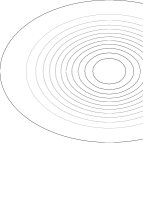
$(0,0)_{++}$           $(0,0)_{-+}$

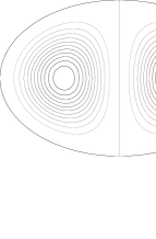
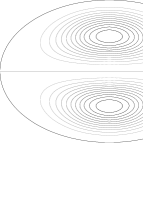
$(0,0)_{+-}$           $(0,0)_{--}$

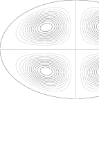
Figure 4: Contourplots of the probability density of the wave functions for the four different parity states $(\pi_{x},\pi_{y})$ for quantum numbers $(r,l)=(0,0)$ and with $a=0.7$. The contourlines are equally spaced from 0 to the maximum probability density of the wave function.

We define the radial quantum number $r$ as the number of zeroes of $F(\rho)$ in the range $\rho\in(0,\rho_{\text{max}})$, i.e. not counting the zeroes at the boundaries. Similarly the angular quantum number $l$ gives the number of zeroes of $G(\phi)$ in the range $\phi\in(0,\pi/2)$, again not counting possible zeroes at the boundaries. This choice of quantum numbers is consistent with the EBK quantization (1) for the symmetry reduced system. Therefore it does not directly give the number of nodes of the wave functions in the full system: depending on the parity there are 0, 1, 2 or 3 additional zeroes in the range $[0,\pi]$ for the states with parity $++$, $-+$, $+-$, and $--$, respectively, such that the total number of angular nodes is $4l+2-\pi_{x}-\pi_{y}$. The energy eigenvalues for the four states with the same quantum numbers are in the same order. In general we denote a state by $(r,l)_{\pi_{x}\pi_{y}}$. Note that the four different parity combinations correspond to the description of the symmetry reduced quarter billiard, where on the coordinate axes Dirichlet (parity $-1$) or Neumann (parity $+1$) boundary conditions are required. To illustrate the symmetries, the probability density of the $(0,0)$ state for each parity is shown in Fig. 4.

The transformation $\cos\phi=\eta$ and $\cosh\rho=\xi$ gives the algebraic form of the Mathieu equation

$$(1-\eta^{2})\partial^{2}_{\eta}g-\eta\partial_{\eta}g+(\lambda-c^{2}\eta^{2})g = 0$$ (12)

$$(1-\xi^{2})\partial^{2}_{\xi}f-\xi\partial_{\xi}f+(\lambda-c^{2}\xi^{2})f = 0\ ,$$ (13)

from which it is obvious that the angular and the radial equation are actually the same, only evaluated on different ranges of the independent variable, $\eta\in[-1,1]$, $\xi\in[1,1/a]$. This equation, although it has regular singular points at $\xi,\eta=\pm 1$, is better suited for the numerical solution of the eigenvalue problem. The requirement for the solution to be smooth at these points replaces the periodic boundary condition.

The Mathieu equation is a special case of the spheroidal wave equation,

$$(1-x^{2})\partial^{2}_{x}h_{m}-2(m+1)x\partial_{x}h_{m}+(\lambda-1/4-m(m+1)-c^{2}x^{2})h_{m}=0\ ,$$ (14)

which appears in the case of the billiard inside the rotational symmetric ellipsoid; $m$ is the quantum number of the angular momentum of rotation around the axis of symmetry. With $m=-1/2$ in (14) we reobtain (12) and (13). We will see that $m=+1/2$ also produces solutions of the Mathieu equation.

In order to obtain solutions with $\pi_{y}=-1$, which must be zero at $\phi=0,\pi$, we must construct solutions which are zero at the regular singular points. It is necessary to factor out this behavior by the ansatz $g(x)=\sqrt{1-x^{2}}h_{1/2}(x)$, $f(x)=\sqrt{x^{2}-1}h_{1/2}(x)$, which transforms (12) and (13) into the equation

$$(1-x^{2})\partial^{2}_{x}h_{1/2}-3x\partial_{x}h_{1/2}+(\lambda-1-c^{2}x^{2})h_{1/2}=0,$$ (15)

which again is a special case of the spheroidal wave equation (14), in this case corresponding to $m=+1/2$, however.

In Fig. 5 four solutions of (14) are shown. The radial and the angular part smoothly join at the regular singular point at $x=1$. We conclude that the spectrum of the 2-dimensional billiard is obtained from the spectrum of the 3-dimensional rotational symmetric billiard if the angular quantum number $m$ in the spheroidal wave function is set to a half integer “spin” number $\pm 1/2$ instead of to an integer number as in the 3-dimensional problem.

Figure 5: The solutions of (14) for the state $r=1$, $l=4$ with the four possible parities, i.e. even or odd at $x=0$ ($\pi_{x}$) and $m=-1/2$ for $\pi_{y}=1$ or $m=1/2$ for $\pi_{y}=-1$; $a=0.7$.

In the standard theory of the Mathieu equation $c$ is fixed and the eigenvalue $\lambda$ is determined. In the billiard problem we have to simultaneously satisfy also the boundary condition for the radial equation. Since both separation constants $\lambda$ and $c^{2}$ appear in each equation, although the variables are separated, the separation constants are not separated, see e.g. [26], which requires a nonstandard approach to the numerical solution of this Sturm-Liouville eigenvalue problem. For the angular equation (12) we have boundary conditions at $\eta=-1$ and at $\eta=0$, corresponding to $\phi=\pi$ and $\phi=3\pi/2$, for the radial equation at $\xi=1$ and $\xi=1/a$, corresponding to $\rho=0$ and to the billiard boundary. Introducing a new independent variable by $\xi=1/a+\zeta(1/a-1)$, the ranges of $\zeta$ and $\eta$ coincide, and we can use a standard shooting method as, e.g., described in [27], to solve both coupled eigenvalue problems simultaneously. Even though the final solution is smooth, as shown in Fig. 5, it is not possible to numerically integrate through the singularity. Instead the integration always starts an epsilon away from the singularity with an analytically calculated regular initial velocity [27]. In order to find a specific state it is necessary to have a fairly good initial guess for the eigenvalues, otherwise the shooting method might converge to another state. We calculate the initial guess via the uniform WKB approach described in the next section, and have found that this always works. The results of these computations are shown in Fig. 6, and some eigenvalues are listed in Tab. III.

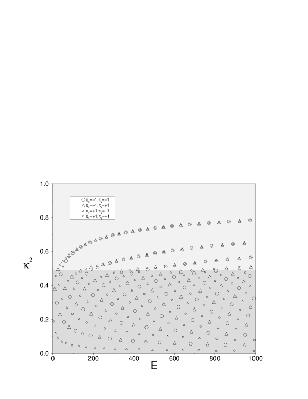
Figure 6: The eigenvalues $(E,\kappa^{2})$ of the eigenstates of the elliptic billiard with $a=0.7$. The region of type $R$ states (rotational, $\kappa^{2}>a^{2}$) is shown in light grey, type $O$ states (oscillating, $\kappa^{2}<a^{2}$) in dark grey.

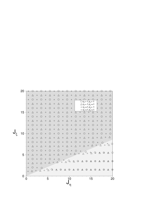
Figure 7: The classical actions ${\mbox{\boldmath$J$\unboldmath}}=2{\mbox{\boldmath$\tilde{I}$\unboldmath}}$ in units of $\hbar$ corresponding to the exact quantum mechanical eigenstates in the elliptic billiard for $a=0.7$. Except for states close to the separatrix, they are located on a lattice given by EBK quantization. The structure near the separatrix can be explained by uniform WKB quantization. Grey code as in Fig. 6.

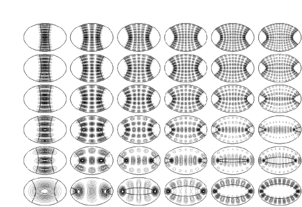
Figure 8: Contourplots of the probability densities of the wavefunctions $(r,l)_{++}$ of the elliptic billiard with $a=0.7$. The vertical axis shows $r=0,\ldots,5$ and the horizontal axis shows $l=0,\ldots,5$. The classical caustic corresponding to the second eigenvalue is also shown.

In Fig. 8 a few symmetric wavefunctions are illustrated. The wave functions for the other parities are related to the $++$ states show in Fig. 8 as illustrated in Fig. 4. In the left column the localization around the stable isolated periodic orbits is clearly visible. It becomes stronger when $r$ is increased. In the bottom row the same happens for the orbit $o_{b}$. Both cases can be explained by considering the WKB wavefunctions for the corresponding states, which is exponentially small outside the classical caustics and nonzero inside. Although the WKB wavefunction diverges at the classical caustic it is correct insofar as the quantum probability density is relatively high close to (and inside) the classical caustic, as can be seen e.g. for the $(4,4)_{++}$ state. The surprising fact, which can not be explained by the above reasoning, is the localization around the focus points, e.g. in the $(1,4)_{++}$ state. This phenomenon occurs at the transition from the rotational states (classical caustic type $R$) to oscillating states (classical caustic type $O$), i.e. close to the classical separatrix. Eigenstates with higher quantum numbers can show even stronger localization around the foci, because their second eigenvalue can be found closer to the critical value $\kappa=a=0.7$. Besides this very strong localization on the focus points these states also show a “scar” [28] of the unstable orbit, e.g. see the $(2,5)_{++}$ state. Although the probability density is low compared to the one in the focus points, it is high compared to the region further away from the $x$-axis. The behaviour outside the foci can again be explained by the WKB wave function, which diverges for $y=0$ for the critical value $\kappa=0.7$. We conclude that in the integrable elliptic billiard states localize around stable periodic orbits, and they also show “scars” along the unstable periodic orbit, with an additional strong localization on the focus points of the ellipse.

The oscillating states of type $O$ are always non-degenerate. The rotational states of type $R$ become more and more degenerate when the distance from the separatrix is increased. The classical reason for this increasing degeneracy is the fact that there are two tori for fixed constants of motion, connected via time reversal symmetry. In a simple EBK quantization these states would be exactly degenerate. Two type $R$ states with the same $r$ and $l$ become (approximately) degenerate if they have period $2\pi$, i.e. if $\pi_{x}\pi_{y}=-1$. If, however, the period is $\pi$, $\pi_{x}\pi_{y}=1$, two states with the same $r$ but $l$ differing by 1 become degenerate. This is consistent with the fact that the total number of nodes on the circle $\phi\in[0,2\pi)$ is $4l+2-\pi_{x}-\pi_{y}$, which gives the same number for the degenerate states. The shift from degenerate states of type $R$ to non-degenerate states of type $O$ can most clearly be seen if the exact quantum eigenvalues $E$, $\kappa^{2}$ are transformed into the classical action space using equations (2) and (2), see Fig. 7. In order to represent the actions of the full system for both types of motion in one picture in such a way that on average one state occupies a box of size $\hbar^{2}$, we use the doubled action of the symmetry reduced billiard ${\mbox{\boldmath$J$\unboldmath}}=2{\mbox{\boldmath$\tilde{I}$\unboldmath}}$. This amounts to doubling the action $I_{\rho}$ for type $R$ tori, which can be understood from two facts: firstly there are two classical tori with the same action for type $R$ tori and secondly the corresponding quantum mechanical states are degenerate in the EBK approximation. The type of movement that each parity state can perform in its “semiclassical quantum cell” will become clear in the next section.

4 Uniform WKB quantization

Consider a Hamiltonian $H=p^{2}/2+V(q)$ with a potential as e.g. given by the effective potentials of sec. 2, see Fig. 1. Let $V(q)<E$ for $q<q_{1}$ and $q>q_{2}$ and $V(q)>E$ in the range $q_{1}<q<q_{2}$. The WKB solutions to the left ($j=1$) and to the right ($j=2$) of the potential barrier are

$$\psi_{j}(q)=\left(A_{j}^{+}\exp(iS_{j}(q)/\hbar)+A_{j}^{-}\exp(-iS_{j}(q)/\hbar)\right)/\sqrt{p(q)}\,,$$ (16)

where

$$p(q)=\sqrt{2\left(E-V(q)\right)},\qquad S_{j}(q)=\int_{q_{j}}^{q}p(q^{\prime})\,dq^{\prime}\,.$$ (17)

The matrix connecting the constants $A_{1}^{+}$ and $A_{1}^{-}$ to $A_{2}^{+}$ and $A_{2}^{-}$ (see e.g. the review of Berry and Mount [14] and the references therein) is given by

$$\begin{array}[]{cc}\left(\begin{array}[]{c}A_{2}^{+}\\ A_{2}^{-}\end{array}\right)=M\left(\begin{array}[]{c}A_{1}^{+}\\ A_{1}^{-}\end{array}\right),&M=e^{\Theta/\hbar}\left(\begin{array}[]{cc}\sqrt{1+e^{-2\Theta/\hbar}}&-i\\ i&\sqrt{1+e^{-2\Theta/\hbar}}\\ \end{array}\right)\,,\end{array}$$ (18)

with the penetration integral $\Theta=-i\int_{q_{1}}^{q_{2}}p(q^{\prime})\,dq^{\prime}$. In the terminology of sec. 2 this is $i$ times the action of an imaginary complex tunneling orbit. This formula is also valid in the case where the energy $E$ lies everywhere above the potential $V(q)$. Then the classical turning points become complex ($q_{1}$ complex conjugate to $q_{2}$) and the penetration integral $\Theta$ becomes negative, corresponding to an imaginary complex scattering orbit. In a potential with several turning points in each region away from the classical turning points a WKB wave function is reasonable. In classically forbidden regions the phase $S$ becomes complex leading to a real exponential. Uniform semiclassical quantization conditions may be obtained by a piecewise connection of these wave functions, and by imposing the correct boundary conditions, e.g. an exponential decay in classically forbidden regions, periodic boundary conditions in the case of a rotor with a potential, or Dirichlet conditions in the case of a hard potential wall, e.g. in a billiard. The resulting quantization conditions take into account real tori and imaginary complex orbits.

The quantization conditions for the planar elliptic billiard are obtained from the effective potentials shown in Fig. 1. We allow for negative values of $\rho$, which can formally be achieved by letting $\phi$ vary between $0$ and $\pi$ only. This is helpful in order to incorporate the different parities (see the boundary conditions in Tab. I) in the semiclassical wave functions $F_{j}(\rho)$ (Eq. (16) for the radial degree of freedom). The wave functions $F_{j}(\rho)$ are symmetric or antisymmetric with respect to $\rho=0$, corresponding to $\pi_{y}=+1$ or $\pi_{y}=-1$ (see Tab. I), consequently

$$\begin{array}[]{ccc}\left(\begin{array}[]{c}A^{+}_{2}\\ A^{-}_{2}\\ \end{array}\right)&=&\pi_{y}\left(\begin{array}[]{cc}0&1\\ 1&0\\ \end{array}\right)\par\left(\begin{array}[]{c}A^{+}_{1}\\ A^{-}_{1}\\ \end{array}\right)\ .\\ \end{array}$$ (19)

The matrix $P$ describes the phase shift along the classically allowed region

$$P=\left(\begin{array}[]{cc}e^{i\frac{\pi}{2}J_{\rho}/\hbar}&0\\ 0&e^{-i\frac{\pi}{2}J_{\rho}/\hbar}\\ \end{array}\right)\,,$$ (20)

where it is important not to use the action $I_{\rho}$ of the full billiard, because this quantity jumps by a factor of 2 as the effective energy increases beyond the top of the barrier. Instead we use ${\mbox{\boldmath$J$\unboldmath}}=2{\mbox{\boldmath$\tilde{I}$\unboldmath}}$ as introduced in the last section, such that the phase shift is continuous at the transition from type $O$ to type $R$ motion. Inserting the Dirichlet boundary conditions $F_{1}(\rho_{0})=F_{2}(\rho_{3})=0$ into (16) leads to

$$\begin{array}[]{cc}\left(\begin{array}[]{c}A^{+}_{1}\\ A^{-}_{1}\\ \end{array}\right)\propto P\left(\begin{array}[]{c}1\\ -1\\ \end{array}\right),\qquad\left(\begin{array}[]{c}A^{+}_{2}\\ A^{-}_{2}\\ \end{array}\right)\propto P^{-1}\left(\begin{array}[]{c}1\\ -1\\ \end{array}\right)\\ \end{array}\,.$$ (21)

The fourth relation among the constants $A_{i}$ is given by (18), where the barrier penetration integral $\Theta=\Theta_{\rho}$ is calculated from one turning point to the other and is given by

$$\Theta_{\rho}=\left\{\begin{array}[]{cl}-2\sqrt{2E}\kappa\left({\cal E}(\sqrt{1-{a^{2}}/{\kappa^{2}}})-{\cal K}(\sqrt{1-{a^{2}}/{\kappa^{2}}})\right)&{\rm type\;}TR\\ -2\sqrt{2E}a\left({\cal E}(\sqrt{1-{\kappa^{2}}/{a^{2}}})-\frac{\kappa^{2}}{a^{2}}{\cal K}(\sqrt{1-{\kappa^{2}}/{a^{2}}})\right)&{\rm type\;}TO\\ -2\sqrt{2E}\sqrt{a^{2}-\kappa^{2}}{\cal E}(a/\sqrt{a^{2}-\kappa^{2}})&{\rm type\;}TO_{c}\ .\end{array}\right.$$ (22)

The action of imaginary complex orbits of type $TO_{c}$ will be needed in the next section.

Composing the connection formula (18), the symmetry (19) and the boundary conditions (21) gives

$$\begin{array}[]{ccc}PMP\left(\begin{array}[]{c}1\\ -1\\ \end{array}\right)&=&\pi_{y}\left(\begin{array}[]{c}-1\\ 1\\ \end{array}\right)\ .\\ \end{array}$$ (23)

Decomposing this complex Equation into its real and imaginary part we obtain the quantization conditions for the radial degree of freedom,

$$\cos{(\pi J_{\rho}/\hbar)}=\frac{-\pi_{y}}{\sqrt{1+e^{2\Theta_{\rho}/\hbar}}}$$ (24)

and

$$\sin{(\pi J_{\rho}/\hbar)}=\frac{-1}{\sqrt{1+e^{-2\Theta_{\rho}/\hbar}}}\ ,$$ (25)

which have to be fulfilled simultaneously. The second Equation is not independent of the first one, it just selects half the number of the solutions of the first Equation.

For the WKB wave function $G(\phi)$ we use $V_{\text{eff}}(\phi)$ (Fig. 1b), and we impose periodic boundary conditions. Following the calculations of Miller [12] for the different parities we obtain the quantization conditions

$$\cos{(\pi J_{\phi}/\hbar)}=\frac{\pi_{x}\pi_{y}}{\sqrt{1+e^{2\Theta_{\phi}/\hbar}}}$$ (26)

and

$$\sin{(\pi J_{\phi}/\hbar)}=\frac{\pi_{x}}{\sqrt{1+e^{-2\Theta_{\phi}/\hbar}}}\ ,$$ (27)

with $\Theta_{\phi}=-\Theta_{\rho}$. The equivalence of the absolute values of $\Theta_{\rho}$ and $\Theta_{\phi}$ is a result of the especially symmetric separation of the Hamiltonian (5). The condition in Eq. (27) just selects the $x$-parity of the solutions of (26).

In Table II the limiting cases for large $|\Theta|$ of the right hand sides of the Equations (24-27) are given. The resulting EBK quantization conditions for the full billiard with quantum numbers $(n_{\rho},n_{\phi})$ and the connection to the quantum numbers $(r,l)$ of the symmetry reduced billiard are indicated. For type $R$ motion these conditions are equivalent to the EBK quantization conditions for the circular billiard.

Eq.	type $O$: $\Theta_{\rho}=-\Theta_{\phi}\ll 0$			type $R$: $\Theta_{\rho}=-\Theta_{\phi}\gg 0$
(24)	$-\pi_{y}$		$I_{\rho}=J_{\rho}=(n_{\rho}+4/4)\hbar$	$0$		$I_{\rho}=J_{\rho}/2=(n_{\rho}+3/4)\hbar$
(25)	$0$	$\bigg{\}}$	$n_{\rho}=2r+(1-\pi_{y})/2$	$-1$	$\bigg{\}}$	$n_{\rho}=r$
(26)	$0$		$I_{\phi}=J_{\phi}=(n_{\phi}+2/4)\hbar$	$\pi_{x}\pi_{y}$		$I_{\phi}=\pm J_{\phi}=\pm n_{\phi}\hbar$
(27)	$\pi_{x}$	$\bigg{\}}$	$n_{\phi}=2l+(1-\pi_{x})/2$	$0$	$\bigg{\}}$	$n_{\phi}=2l+(2-\pi_{x}-\pi_{y})/2$

Table II: The limiting cases of the right hand sides of the Equations (24-27). The quantum numbers for the corresponding EBK quantization conditions are $n_{\rho},n_{\phi}\in{\mathbb{N}}\cup\{0\}$ for the full system and $r,l\in{\mathbb{N}}\cup\{0\}$ for the desymmetrized billiard.

How to calculate the $(E,\kappa^{2})$- or the $(J_{\rho},J_{\phi})$-spectrum from the conditions in Eq. (24), (25), (26) and (27)? The actions and the barrier penetration integrals are functions of $(E,\kappa^{2})$. With Newton’s method we can numerically obtain $(E,\kappa^{2})$ as functions of $(J_{\rho},J_{\phi})$ and therefore $\Theta_{\rho}$ and $\Theta_{\phi}$ as functions of $(J_{\rho},J_{\phi})$. Ignoring (25) and (27) for the moment, the remaining Equations (24) and (26) can thus be rewritten in the form

$$\begin{array}[]{lllrl}f^{\pi_{y}}_{1}(J_{\rho},J_{\phi})&:=&\cos{(\pi J_{\rho}/\hbar)}+\pi_{y}g_{1}(\Theta_{\rho}(J_{\rho},J_{\phi}))&=&0\\ f_{2}^{\pi_{x},\pi_{y}}(J_{\rho},J_{\phi})&:=&\cos{(\pi J_{\phi}/\hbar)}-\pi_{x}\pi_{y}g_{2}(\Theta_{\phi}(J_{\rho},J_{\phi}))&=&0\ ,\end{array}$$ (28)

where $g_{1}$ and $g_{2}$ are smooth functions onto the intervall $(0,1)$. A solution of (28) can be viewed as an intersection of the lines $f_{1}^{\pi_{y}}=0$ and $f_{2}^{\pi_{x},\pi_{y}}=0$ in action space with the same corresponding parities. The solutions lie inside a box with the edges defined by the extremal values of $g_{1}$ and $g_{2}$. Because of the periodicity of the left hand sides of Equations (24-27) these boxes are always arranged in the same way inside a cell in the $(J_{\rho},J_{\phi})$-space. We call these quadratic cells “semiclassical quantum cells” with quantum numbers $(r,l)$. Their edges have length $\Delta J_{\rho}=\Delta J_{\phi}=2\hbar$ and they tessellate the whole $(J_{\rho},J_{\phi})$-space. Inside a quantum cell there are four quantum states, one for each parity. Each state of fixed parity is confined to a “parity box” of width $\hbar/2$, shown by bold lines in Fig. 9. The size of the parity box is a result of the fact that the Maslov indices change by two upon the transition of the separatrix, see Tab. II These parity boxes take care of the remaining conditions (25) and (27): inside a box they are automatically fulfilled when (28) holds. To find the solution guaranteed to lie in the interior of a box, we use the bisection method described in [29]. Having got all solutions in action space, we compute again the solutions in $(E,\kappa^{2})$-space with Newton’s method to obtain the semiclassical eigenvalue spectrum. Introducing the semiclassical quantum cells in action space ensures that always the right state is found, even when two states are almost degenerate. The method can easily be extended to the case of more than two degrees of freedom.

Figure 9: Schematic view of the four states in a single semiclassical quantum cell $(\Delta J_{\rho}=\Delta J_{\phi}=2\hbar)$ for (a) the region $R$, (b) the region $O$ and (c) close to the separatrix corresponding to the states with quantum numbers $(0,1)$. The intersections of the lines $f_{1}^{\pi_{y}}=0$ and $f_{2}^{\pi_{x},\pi_{y}}=0$ with equal parities (dots) are the solutions of the quantization conditions (24), (25), (26) and (27) if they are located inside a parity box. The squares and the triangles are the states obtained from EBK quantization in regions $R$ and $O$, respectively. Parity boxes that are crossed by the bold dashed separatrix may contain two EBK states (bold squares and triangles) or no EBK states, because both corners (the thin squares and triangles) are in the wrong region. The EBK Maslov index is $(3,0)$ in region $R$ (where $J_{\rho}=2I_{\rho}$) and $(4,2)$ in region $O$.

Figure 11 and Tab. III show the result of the semiclassical calculation compared to the exact quantum mechanical results. The distinction between the parities is omitted in Fig. 11 because this becomes already clear from Fig. 7. In Fig. 10 the relative errors of the semiclassical eigenvalues $(E_{\text{qm}}-E_{\text{sc}})/E_{\text{qm}}$ and $(\kappa_{\text{qm}}-\kappa_{\text{sc}})/\kappa_{\text{qm}}$ are plotted versus $\kappa_{\text{qm}}$, such that the behavior of the error with respect to the position of the state on the classical energy surface can be seen. The semiclassical energy eigenvalues are almost always too low, see also Tab. III. The opposite holds for the values of the second eigenvalue, which usually are too high. The only exception (for both eigenvalues) occurs in the neighborhood of the classical separatrix. The fact that Fig. 10 looks rather symmetric indicates that the relative errors of the two eigenvalues are strongly correlated. Concerning the semiclassical limit we see series of states with increasing $r$ quantum number and decreasing error for small $\kappa$, and series with increasing $l$ quantum number and decreasing error for large $\kappa$. However, increasing $l$ with $\kappa<a$ does not decrease the error. The error of the whispering gallery states $(0,l)$ is particularly large. In general, however, the agreement between the exact eigenvalues and the semiclassical values is very good.

Figure 10: The relative error of semiclassical energy eigenvalue (circles) and $\kappa$ eigenvalue (pluses) plotted versus $\kappa$. The obvious patterns result from series of states with the indicated quantum numbers. The arrows point into the direction of increasing quantum number.

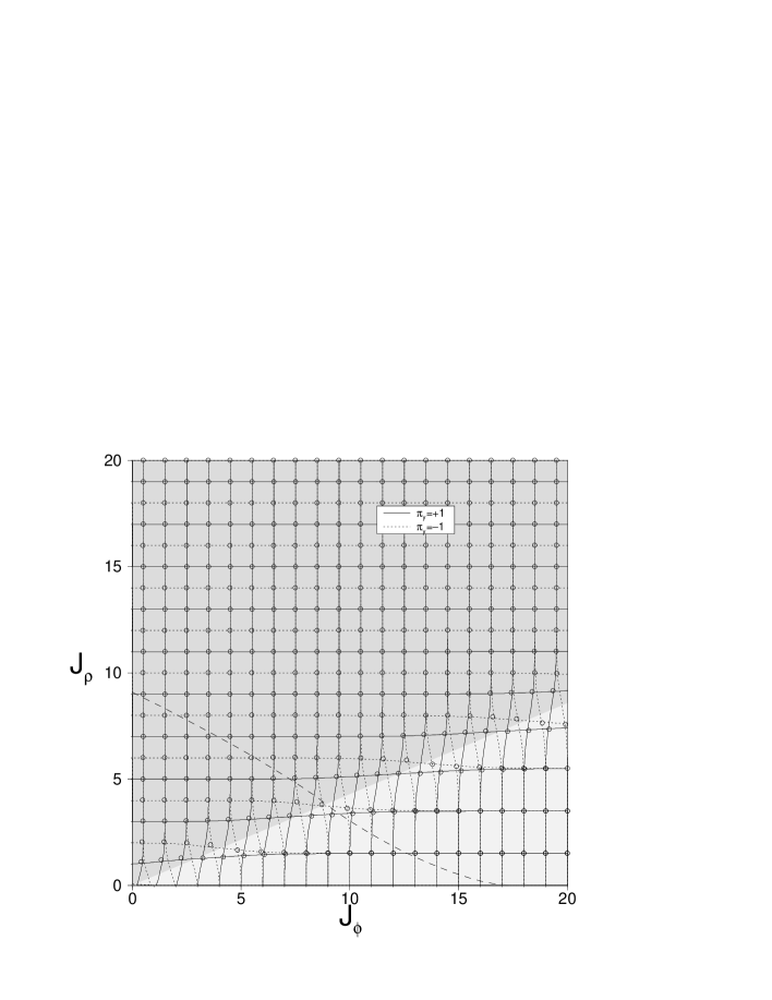
Figure 11: Comparison of the exact states (circles) to the semiclassical states (intersections of the lines $f_{1}^{\pi_{y}}=0$ and $f_{2}^{\pi_{x},\pi_{y}}=0$ with the same corresponding parities). The dashed line is the energy surface $E=200$. $J_{\rho}$ and $J_{\phi}$ are measured in units of $\hbar$.

$E_{{\text{qm}}}$	$\kappa^{2}_{{\text{qm}}}$	$E_{{\text{sc}}}$	$\kappa^{2}_{{\text{sc}}}$	$r$	$l$	$\pi_{x}$	$\pi_{y}$
4.26746	0.18714	3.99539	0.21120	0	0	+	+
9.05834	0.37981	8.65488	0.39821	0	0	$-$	+
12.5768	0.12960	12.3295	0.13666	0	0	+	$-$
15.9933	0.45667	15.5268	0.46827	0	1	+	+
19.3576	0.30380	18.9734	0.31216	0	0	$-$	$-$
25.0613	0.49625	24.7502	0.49755	0	1	$-$	+
25.8947	0.09212	25.6683	0.09516	1	0	+	+
⋮
1000.46	0.13551	1000.21	0.13560	8	2	+	$-$
1001.65	0.65621	1000.78	0.65650	1	13	$-$	$-$
1001.65	0.65621	1000.78	0.65650	1	14	+	+
1002.01	0.43314	1001.40	0.43342	5	8	+	+
1008.07	0.19149	1007.80	0.19159	8	3	+	+
1010.97	0.36819	1010.52	0.36838	6	6	$-$	+
1013.91	0.48076	1012.72	0.48148	4	9	$-$	+
1018.48	0.24440	1018.17	0.24451	7	4	+	$-$
1029.35	0.78842	1026.76	0.78970	0	16	+	$-$
1029.35	0.78842	1026.76	0.78970	0	16	$-$	+

Table III: The quantum mechanical eigenvalues $(E_{{\text{qm}}},\kappa^{2}_{{\text{qm}}})$ and the semiclassical eigenvalues $(E_{{\text{sc}}},\kappa^{2}_{{\text{sc}}})$ of the billiard in the ellipse for $a=0.7$ with $E_{{\text{qm}}}<26$ or $1000<E_{{\text{qm}}}<1030$.

Now we study the change of the regular lattice obtained from EBK quantization induced by the uniformization. There are three typical situations in action space represented in Fig. 9: region $R$ (a) and region $O$ (b) both far away from the separatrix and the region close to the separatrix (c). In region $R$ the EBK states $(r,l+1)_{++},(r,l)_{--}$ (e.g. Tab. III rows 9 and 10) and $(r,l)_{+-},(r,l)_{-+}$ (e.g. rows 16 and 17) are almost degenerate. This corresponds to the degeneration of clockwise and counterclockwise rotations in the planar circular billiard. The EBK states form regular lattices, with mesh size $\Delta J_{\rho}=2\hbar$ and $\Delta J_{\phi}=\hbar$ with two states on each corner in region $R$ and $\Delta J_{\rho}=\Delta J_{\phi}=\hbar$ in region $O$. Far away from the separatrix the uniform semiclassical states lie near the EBK states with Maslov index $(3,0)$ for type $R$ and $(4,2)$ for type $O$. Approaching the separatrix a transition between the two regular EBK lattices takes place. Crossing the separatrix from region $R$ to region $O$ the shift of the EBK states is $\delta J_{\rho}=-\hbar/2$ and $\delta J_{\phi}=\hbar/2$ for $\pi_{y}=+1$ and $\delta J_{\rho}=\hbar/2$ and $\delta J_{\phi}=-\hbar/2$ for $\pi_{y}=-1$. The uniform quantization smoothly joins the EBK lattices along the separatrix. It is natural to interpret the location of the semiclassical states as two separate meshes: one for $\pi_{y}=+1$ and one for $\pi_{y}=-1$, indicated by full and dotted lines in Fig. 11.

Figure 9c shows that close to the separatrix not only the accuracy of the EBK states is unsatisfactory but also that EBK quantization sometimes yields a wrong number of states. In Fig. 9c the situation for the $(0,1)$-quantum cell is shown. The EBK states are marked by bold squares in region $R$ and by bold triangles in region $O$. A square represents two EBK states because of the degeneracy in region $R$. The $+-$ parity box contains one EBK state, marked by the bold triangle. The opposite corner of this parity box could be reached with the Maslov index defined for region $R$. However, it is located on the wrong side of the separatrix, and therefore not a true EBK state indicated by a thin square. By the same reasoning the parity boxes $++$ and $-+$ contain no true EBK state. On the contrary the $--$ parity box contains two true EBK states. This indicates the main deficiency of EBK quantization for systems that exhibit a separatrix.

5 The Berry-Tabor trace formula

In the last section we have seen how the imaginary complex orbits lead to a Maslov index smoothly varying across the separatrix. The real complex orbits can be taken into account by a completely different approach introduced by Berry and Tabor [15]. The goal of this section is to incorporate the imaginary complex orbits into the Berry-Tabor trace formula, such that all kinds of classically forbidden tori are taken into account.

Starting from EBK quantization Berry and Tabor derived a formula for the semiclassical density of states

$$n_{\text{s}c}(E)=\sum_{{\mbox{\boldmath$n$\unboldmath}}}\delta\left(E-H(({\mbox{\boldmath$n$\unboldmath}}+\frac{{\mbox{\boldmath$\alpha$\unboldmath}}}{4})\hbar)\right)$$ (29)

in terms of resonant tori for an integrable system with $f$ degrees of freedom. They transformed Eq. (29) via the Poisson summation formula and performed the integrals in stationary-phase approximation. The result is

$$n_{\text{s}c}(E)=\overline{n}(E)+\frac{2}{\hbar^{\frac{f+1}{2}}}\sum\limits_{\mbox{\boldmath$\mu$\unboldmath}}\frac{1}{|{\mbox{\boldmath$\omega$\unboldmath}}({\mbox{\boldmath$I$\unboldmath}}^{\mu})||{\mbox{\boldmath$\mu$\unboldmath}}|^{\frac{f-1}{2}}\sqrt{|C({\mbox{\boldmath$I$\unboldmath}}^{\mu})|}}\sum\limits^{\infty}_{q=1}\frac{\cos{(q(S({\mbox{\boldmath$I$\unboldmath}}^{\mu})/\hbar-\frac{\pi}{2}{\mbox{\boldmath$\alpha$\unboldmath}}{\mbox{\boldmath$\mu$\unboldmath}})+\frac{\pi}{4}\beta)}}{q^{\frac{f-1}{2}}}.$$ (30)

The first summation is over all relatively prime non-negative integers $\mu$, i.e. over families of prime orbits, while the second summation runs over all their repetitions. The Maslov indices are always the same since the energy surface is assumed to have no separatrix. The term ${\mbox{\boldmath$\mu$\unboldmath}}=0$ is excluded from the sum and denoted by $\overline{n}(E)$; it gives the mean density of states, the so-called Thomas-Fermi term. For the elliptic billiard we have $\overline{n}(E)=A_{b}/(2\pi\hbar^{2})$ according to Weyl’s law where $A_{b}=\pi\sqrt{1-a^{2}}$ gives the billiard’s area. In [19] it is shown that next order correction to Weyl’s law, proportional to the circumference of the billiard, is contained in the whispering gallery orbits in the remaining sum.

To improve the convergence of the series (30) it is advantageous to introduce a smoothed density of states $n_{\text{s}c}(E;\gamma)$ by giving $E$ a small imaginary part $i\gamma$. Then a $\delta$-peak changes into a Lorentz function with half width energy $\gamma$. The semiclassical formula for $n_{\text{s}c}(E;\gamma)$ differs from formula (30) by a decay factor $D=\exp{(-\gamma qT({\mbox{\boldmath$I$\unboldmath}}^{\mu})/\hbar)}$ before the cosine term in the second summation.

Berry and Tabor show that formula (30) can be improved by taking into account resonant real complex tori. This removes unphysical discontinuities in the density of states resulting from contributions of resonant tori which are suddenly classically realized as $E$ changes. For a system that scales with respect to the energy this cannot occur, nevertheless the system parameter $a$ can take over the role of the energy, e.g. for the elliptic billiard all real complex orbits become realized for $a\to 1$. Even without a parameter these corrections are sensible because they improve the situation when the stationary phase approximation is bad because there is a stationary point close to, but outside the range of integration. The resulting trace formula incorporating real complex orbits for two degrees of freedom systems reads

$$\begin{array}[]{r}n_{\text{s}c}(E;\gamma)=\overline{n}(E)+\frac{2}{\hbar^{3/2}}\sum\limits_{\mbox{\boldmath$\mu$\unboldmath}}\frac{1}{|{\mbox{\boldmath$\omega$\unboldmath}}({\mbox{\boldmath$I$\unboldmath}}^{\mu})|\sqrt{|{\mbox{\boldmath$\mu$\unboldmath}}||C({\mbox{\boldmath$I$\unboldmath}}^{\mu})|}}\sum\limits^{\infty}_{q=1}D\;A\frac{\cos{(q(S({\mbox{\boldmath$I$\unboldmath}}^{\mu})/\hbar-\frac{\pi}{2}{\mbox{\boldmath$\alpha$\unboldmath}}{\mbox{\boldmath$\mu$\unboldmath}})+\theta)}}{\sqrt{q}}\\ -\frac{2}{\sqrt{2\pi}\beta\hbar}\sum\limits_{\mbox{\boldmath$\mu$\unboldmath}}\frac{1}{|{\mbox{\boldmath$\omega$\unboldmath}}({\mbox{\boldmath$I$\unboldmath}}^{\mu})|\sqrt{|{\mbox{\boldmath$\mu$\unboldmath}}||C({\mbox{\boldmath$I$\unboldmath}}^{\mu})|}}\sum\limits^{\infty}_{q=1}D\left(\frac{\sin{(q(S_{2}/\hbar-\frac{\pi}{2}{\mbox{\boldmath$\alpha$\unboldmath}}{\mbox{\boldmath$\mu$\unboldmath}}))}}{\Lambda_{2}\sqrt{q}}-\frac{\sin{(q(S_{1}/\hbar-\frac{\pi}{2}{\mbox{\boldmath$\alpha$\unboldmath}}{\mbox{\boldmath$\mu$\unboldmath}}))}}{\Lambda_{1}\sqrt{q}}\right)\\ +\frac{1}{\pi\hbar}\sum\limits_{\mbox{\boldmath$\mu$\unboldmath}}\sum\limits^{\infty}_{q=1}D\left(\frac{\sin(q(S_{2}/\hbar-\frac{\pi}{2}{\mbox{\boldmath$\alpha$\unboldmath}}_{2}{\mbox{\boldmath$\mu$\unboldmath}}))}{q|{\mbox{\boldmath$\omega$\unboldmath}}_{2}|{\mbox{\boldmath$\mu$\unboldmath}}{\mbox{\boldmath$I$\unboldmath}}^{\prime}_{2}}-\frac{\sin(q(S_{1}/\hbar-\frac{\pi}{2}{\mbox{\boldmath$\alpha$\unboldmath}}_{1}{\mbox{\boldmath$\mu$\unboldmath}}))}{q|{\mbox{\boldmath$\omega$\unboldmath}}_{1}|{\mbox{\boldmath$\mu$\unboldmath}}{\mbox{\boldmath$I$\unboldmath}}^{\prime}_{1}}\right),\end{array}$$ (31)

where $S_{1,2}$ are the actions, ${\mbox{\boldmath$\alpha$\unboldmath}}_{1,2}$ the Maslov indices and ${\mbox{\boldmath$I$\unboldmath}}^{\prime}_{1,2}$ the normalized derivatives with respect to a second constant of motion $\xi$, which parametrizes the energy surface in action space; all quantities with indices $1,2$ are evaluated at the boundaries $\xi_{1}$ and $\xi_{2}$ of the energy surface. $A$ is the amplitude and $\theta$ the argument of the complex Fresnel integral

$$F=\frac{1}{\sqrt{2\pi}}\int^{\Lambda_{2}/\sqrt{\hbar}}_{\Lambda_{1}/\sqrt{\hbar}}dxe^{i\frac{\beta}{2}x^{2}}\ ,$$ (32)

where $\Lambda_{1,2}\in{\mathbb{R}}$ are defined by $\Lambda^{2}_{1,2}=2q/\beta(S_{1,2}-S)$ and $\Lambda_{1,2}\stackrel{{\scriptstyle\scriptscriptstyle>}}{{\scriptscriptstyle<}}0$ if $\xi_{1,2}\stackrel{{\scriptstyle\scriptscriptstyle>}}{{\scriptscriptstyle<}}\xi^{\mu}$, where ${\mbox{\boldmath$I$\unboldmath}}^{\mu}={\mbox{\boldmath$I$\unboldmath}}(\xi^{\mu})$. The series (31) holds for real and real complex tori.

Formulas (30) and (31) can be applied to simple systems [15, 30] but not to systems with separatrices like the elliptic billiard. In the derivation of Berry and Tabor the energy surface is assumed to be strictly convex or strictly concave and to have a smooth curvature. This is not the case for a system with separatrices, e.g. the elliptic billiard, as can be seen in Fig. 2. We are going to study three versions of the Berry-Tabor trace formula with sucessive improvements concerning states close to the separatrix. A first approach, similar to [31], would be to divide the energy surface into smooth patches and to consider (30) or (31) for each patch. We call this the EBKBT quantization. The manifestation of the separatrix in the EBK approximation as a discontinuous quantization condition is carried over to the EBKBT quantization by the appearance of the wrong number of terms in the summation (30) or (31). In the semiuniform WKBBT quantization we correct this deficiency by taking the Maslov index in (29) as a uniform Maslov phase, smoothly varying across the separatrix. However, the new term is considered constant in the stationary phase approximation. This improves the results and still gives a sum over periodic orbits. The best results are obtained if the Maslov phase is fully taken into account in the stationary phase approximation, leading to summation over (in general) non-periodic orbits in a uniform WKBBT trace formula.

The resonant tori of an integrable two degrees of freedom system are characterized by the winding number $w(\kappa^{\mu})=\mu_{\phi}/\mu_{\rho}$. For a billiard system without potential $w$ is independent of the energy. Thus we can obtain all resonant tori for one reference energy. The actions, the frequencies and the reciprocal curvature scale with $\sqrt{E}$. Hence all these quantities must only be calculated for the reference energy. For the elliptic billiard the winding number $w$ is restricted to the interval $(0,1)$. Thus for resonances up to a fixed order we have $0<\mu_{\rho}\leq\mu_{\text{max}}$ and $0<\mu_{\phi}<\mu_{\rho}$. For the summation over $q$, i.e. over the repetitions, we incorporate all orbits with period $qT$ less than a cutoff time $T_{c}=\frac{\hbar}{\gamma}\ln{\frac{2}{\epsilon}}$ to guarantee that the error in the second summation of formula (30) is smaller than $\epsilon$. In the following we choose $a=0.7$, $\hbar=1$, $\gamma=0.3$ and $\epsilon=10^{-8}$. Thus the cutoff time is $T_{c}\approx 63.7$. For numerical reasons it is not possible to approach the cusp of $w$ (see Fig. 2b for $\tilde{w}$) arbitrarily close. We can only include all resonant tori with $|\kappa^{2}-a^{2}|>10^{-14}$, i.e. $\tilde{w}<0.472$ for type $R$ and $\tilde{w}<0.943$ for type $O$. But the contribution of tori with larger winding numbers are very small because of the divergence of the curvature at $\kappa^{2}=a^{2}$. Taking $\mu_{\text{max}}=250$, we include $26\,395$ and neglect $2\,026$ resonant tori in the summation. The remaining interval $[0,2\arccos{(a)}/\pi)\approx[0,0.506)$ carries the real complex tori (type $O_{c}$). Since for $a=0.7$ the real complex torus with $w=1/2$ has the predominant effect we found it sufficient to consider resonant real complex tori with $\kappa^{2}\geq\kappa^{2}_{\text{min}}=-15$, i.e. $w(\kappa)\geq w(\kappa_{\text{min}})=0.285$. Resonant tori with $\kappa^{2}<\kappa^{2}_{\text{min}}$ give negligible constributions, even though the curvature is very small, due to the destructive interference in the Fresnel integral (32). The number of incorporated real complex tori is $4\,205$, $5\,1$ are left out.

In the EBKBT approach we set ${\mbox{\boldmath$\alpha$\unboldmath}}=(3,0)$ and $\beta=1$ for the patch $R$ and ${\mbox{\boldmath$\alpha$\unboldmath}}=(4,2)$ and $\beta=-1$ for patch $O$. On patch $R$ the EBK states are exactly degenerate, thus all the contributions are multiplied by 2. Since there are only real complex tori of type $O_{c}$, in Eq. (31) for patch $O$ we only consider terms corresponding to the boundary $\xi_{1}$ ($\kappa^{2}=0$) and no boundary terms for patch $R$. Figure 12 presents the spectrum $n_{\text{s}c}(E;\gamma)$ calculated with the EBKBT quantization in the range $12.5\leq E\leq 47.5$. For comparison the exact spectrum smoothed in a Lorentzian manner is shown. We focus on the states shown in the quantum cell $(0,1)$ close to the separatrix shown in Fig. 9. The other states in Fig. 12 are reproduced fairly well. First we observe that the $(0,1)_{+-}$ state is also reproduced quite well, which is due to the fact that the corresponding parity cell correctly contains one EBK state only. The peak for the parity box $(0,1)_{++}$ splits into two peaks with approximately half amplitude. The reason is that there is no true EBK state in this parity box. However the two corners of the box carry EBK states located in the wrong region (the thin square and triangle in Fig. 9), and they still give a small contribution in the trace formula. The situation is similar for the $(0,1)_{-+}$ state. Here the EBK peak also splits into two small peaks; one accidently overlaps with the $(1,0)_{++}$ EBK state and the other one is seen as a small bump on the left side. In both cases the EBKBT quantization almost fails to produce a state. The parity box $(0,1)_{--}$ in Fig. 9 contains two EBK states. Since both of them are in the correct region (the bold square and triangle) they both produce peaks with almost the usual amplitude, which can be clearly seen by considering $--$ parity only, i.e. by looking at the billiard in the quarter of an ellipse. In Fig. 12 we instead observe that the $(0,2)_{++}$ peak has almost doubled amplitude: this is the result of the assumed degeneracy of states in the region $R$. So here the EBKBT quantization produces one state too much. The corresponding peaks in the spectrum are called “large spurious peaks” in [31].

Figure 12: Comparison of the exact quantum mechanical density of states (dotted line) to the semiclassical density $n_{\text{s}c}(E;\gamma)$ calculated from EBKBT quantization (solid line). The labels refer to the exact peaks. EBKBT peaks connected to parity boxes with the wrong number of states (see Fig. 9) do not give satisfactory results.

Figure 13: Comparison of the exact quantum mechanical density of states (dotted line) to the semiclassical density $n_{\text{s}c}(E;\gamma)$ calculated with semiuniform WKBBT quantization (solid line). semiuniform WKBBT peaks corresponding to parity boxes with no EBK state at all ($(0,1)_{++}$ and $(0,1)_{-+}$) are improved as compared to Fig. 12. The parity box $(0,1)_{--}$ with two EBK states still produces two peaks.

To remove these problems the tunneling through the potential barriers should be incorporated by a summation over imaginary complex orbits. For one-degree-of-freedom-systems the consideration of tunneling orbits can be done in a simple way [32, 33]. For systems with more degrees of freedom the problem is rather involved. In particular a Green’s function approach in terms of action angle variables is still out of reach except for special systems [34]. Thus we again start with Eq. (29) as Berry and Tabor did. At the heart of their approach are the EBK quantization conditions of the form (1) which allow for a resummation of the semiclassical density of states via Poisson summation. At this stage we allow for a varying $\alpha$ in Eq. (1), i.e. we base our calculations on a uniform quantization condition. Note that this uniformization is completely different from the uniformization of Berry and Tabor, which involves only real complex tori. We incorporate both approaches, with the result that all kinds of classically forbidden tori described in sec. 2 are taken into account.

An effective Maslov phase ${\mbox{\boldmath$\tilde{\alpha}$\unboldmath}}({\mbox{\boldmath$\tilde{I}$\unboldmath}};\pi_{x},\pi_{y})$ varying smoothly on the energy surface can be extracted from Equations (24-27). Inserting the EBK quantization condition (1) into these Equations the quantum number $n$ drops out because it appears as $2\pi n$ in the argument of the trigonometric functions. Thus we obtain the effective Maslov phases as

$$\tilde{\alpha}_{\rho}({\mbox{\boldmath$\tilde{I}$\unboldmath}};\pi_{x},\pi_{y})=\pi_{y}\frac{2}{\pi}\arctan{(e^{\Theta_{\rho}(\tilde{I}_{\rho},\tilde{I}_{\phi})/\hbar})}+3-\pi_{y}$$ (33)

and

$$\tilde{\alpha}_{\phi}({\mbox{\boldmath$\tilde{I}$\unboldmath}};\pi_{x},\pi_{y})=\pi_{y}\frac{2}{\pi}\arctan{(e^{\Theta_{\phi}(\tilde{I}_{\rho},\tilde{I}_{\phi})/\hbar})}+2-\pi_{y}-\pi_{x}\ .$$ (34)

Then we introduce new variables, behaving like continuous quantum numbers

$${\mbox{\boldmath$\tilde{n}$\unboldmath}}=\frac{1}{\hbar}{\mbox{\boldmath$\tilde{I}$\unboldmath}}-\frac{1}{4}{\mbox{\boldmath$\tilde{\alpha}$\unboldmath}}({\mbox{\boldmath$\tilde{I}$\unboldmath}})$$ (35)

for each parity. The energy surfaces in these variables (one for each parity), which now depend on the energy through $\tilde{\alpha}$, are shown in Fig. 14. The energy surfaces with equal $\pi_{y}$ have the same shape, but differ in a horizontal shift by the constant $1/2$. For $\hbar\to 0$ $\tilde{\alpha}$ becomes a step function such that except for a shift and the parity splitting the classical energy surfaces are reobtained in the semiclassical limit. The quantization conditions for these variables read ${\mbox{\boldmath$\tilde{n}$\unboldmath}}\in{\mathbb{N}}^{2}$ and are trivial. In sec. 4 we studied how the lattice of states changes across the separatrix, while the energy surface was the same for all energies. Now we turn the point of view and introduce new variables $\tilde{n}$ giving a trivial lattice but a more complicated energy surface instead. The lines of constant $\tilde{n}_{\rho},\tilde{n}_{\phi}$ in the usual action variables are shown in Fig. 11.

Since the quantization conditions in the new variables are of EBK type, we can repeat the derivation of the trace formula by Berry and Tabor. The phase being approximated in this derivation is $\mu$$\tilde{n}$. Without separatrix the only non constant part in $\tilde{n}$ is $\tilde{I}$, and the stationary phase condition leads to resonant tori. In order to keep the summation over resonant tori we must assume that ${\mbox{\boldmath$\tilde{\alpha}$\unboldmath}}({\mbox{\boldmath$\tilde{I}$\unboldmath}};\pi_{x},\pi_{y})$ varies slowly in action space, which is also the approach followed in [19]. This gives a trace formula with two minor modifications: Firstly each sum is subdivided into separate sums for each parity. Secondly $\tilde{\alpha}$ now is different for every resonant torus. We call this method semiuniform WKBBT quantization. Figure 13 shows the semiuniform WKBBT spectrum for the same parameters as above. The states $(0,1)_{++}$ and $(0,1)_{-+}$ (parity cells without EBK state) are reconstructed in a satisfactory manner. The $(0,1)_{--}$ state (parity cell with two EBK states) has improved, but it still contains two contributions, which is due to the fact that we assume $\tilde{\alpha}$ to be constant in the stationary phase approximation, which is a particularly bad assumption in the neighborhood of the separatrix.

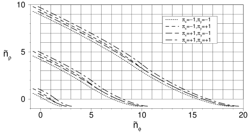
Figure 14: The energy surfaces in the variables $\tilde{n}$ for the energies $25$, $300$, $1026.76$. In contrast to Fig. 11 here the shape of the energy surfaces depends on the energy but the semiclassical states form a regular lattice. For the energy $E=1026.76$ the almost degeneracy of the semiclassical states $(0,16)_{+-}$ and $(0,16)_{-+}$ is shown.

Thus we are finally led to the necessity to fully take into account the variation of $\tilde{\alpha}$. In essence this means to take the surfaces in Fig. 14 as new energy surfaces, and define all quantities (most notably the winding number) with respect to them. Most important, the stationary points are now given by

$${\mbox{\boldmath$\mu$\unboldmath}}\frac{\partial{\mbox{\boldmath$\tilde{I}$\unboldmath}}}{\partial\kappa^{2}}=\frac{\hbar}{4}{\mbox{\boldmath$\mu$\unboldmath}}\frac{\partial{\mbox{\boldmath$\tilde{\alpha}$\unboldmath}}}{\partial\kappa^{2}}=\frac{\Theta^{\prime}}{\cosh\Theta}(\mu_{\phi}-\mu_{\rho})\,.$$ (36)

Although far away from the separatrix $|\Theta|$ is large and this condition almost reduces to the ordinary resonance condition, in general Equations (30) and (31) are no longer summations over resonant tori and consequently the resulting semiclassical density of states is not determined by periodic orbits. Instead the tori to be taken into account in the sum are given by the rational values of a new effective winding number

$$w_{\text{n}}(E,\kappa)=-\frac{\partial\tilde{n}_{\rho}}{\partial\kappa^{2}}\Big{/}\frac{\partial\tilde{n}_{\phi}}{\partial\kappa^{2}}\,,$$ (37)

such that the solutions of Eq. (36) are given by $w_{\text{n}}(E,\kappa)=\mu_{\phi}/\mu_{\rho}$. The overall structure of the trace formula does not change, however, the frequencies and the curvature have to be replaced by the respective expressions obtained from the surface ${\mbox{\boldmath$\tilde{n}$\unboldmath}}(\kappa)$. An important difference between the winding numbers $w$ and $w_{\text{n}}$ is that the latter depends on the energy. This leads to an enormous numerical effort for the calculation of $n_{\text{s}c}(E;\gamma)$, because it is necessary to determine the stationary points for every energy separately. We call this method uniform WKBBT quantization in contrast to the semiuniform WKBBT quantization, since it neglects the varying $\tilde{\alpha}$ in the stationary phase approximation. The uniform WKBBT spectrum calculated with the same parameters as above is shown in Fig. 15. As expected the splitting of the $(0,1)_{--}$ state is now removed. In the evaluation of the sum we define the boundaries of the energy surfaces as ${\mbox{\boldmath$\tilde{n}$\unboldmath}}(\kappa=0)$ and ${\mbox{\boldmath$\tilde{n}$\unboldmath}}(\kappa=1)$. This choice is somewhat arbitrary since one could also define the boundaries as $\tilde{n}_{\rho}=0$ and $\tilde{n}_{\phi}=0$. But we want to focus onto states close to the separatrix where this arbitrariness is not relevant. The little peaks in Fig. 15 are artefacts which could be removed by including larger $\mu$ in the sum.

Figure 15: Comparison of the semiuniform WKBBT density of states (dotted line) to the density calculated with the uniform WKBBT quantization (solid line). The density obtained from the energy eigenvalues calculated in sec. 4 (dashed) gives the expected location of the peak, which is slightly displaced from the peak in the exact quantum mechanical density (long dashed). The main point is that the splitting of the $(0,1)_{--}$ peak is removed.

The derivation of the effective Maslov phase (33) and (34) makes it obvious that in the uniform $\tilde{\alpha}$ the effects of tunneling and scattering orbits are incorporated into the Berry-Tabor sum. Now we want to show that the consideration of an effective $\tilde{\alpha}$ is equivalent to an explicit incorporation of imaginary complex orbits with constant $\tilde{\alpha}$.

We consider two crossed double well potentials, which is slightly more general than the elliptic billiard since the barrier penetration integrals $\Theta_{1}$ and $\Theta_{2}$ are then unrelated. The effective $\tilde{\alpha}$ obtained by the method described in sec. 4 can always be written as $\tilde{\alpha}_{i}=-2\zeta_{i}/\pi+\tilde{\alpha}_{ci}$, with $\zeta_{i}=\arctan{\exp{(-\Theta_{i})}}$ and ${\mbox{\boldmath$\tilde{\alpha}$\unboldmath}}_{c}=(\tilde{\alpha}_{c1},\tilde{\alpha}_{c2})$ is a constant integer vector. We rewrite the cosine term in Eq. (30) with $x=q(S/\hbar-\pi/2{\tilde{\mbox{\boldmath$\alpha$\unboldmath}}_{c}}{{\mbox{\boldmath$\mu$\unboldmath}}})+\pi/4\beta$ and $q_{i}=q\mu_{i}>0$ as the real part of

$$e^{i(x+q_{1}\zeta_{1}+q_{2}\zeta_{2})}=e^{ix}(r_{1}+it_{1})^{q_{1}}(r_{2}+it_{2})^{q_{2}}$$ (38)

with

$$r_{i}=\cos\zeta_{i}=\frac{1}{\sqrt{1+e^{-2\Theta_{i}}}}\;\;\mbox{ and }\;\;t_{i}=\sin\zeta_{i}=\frac{1}{\sqrt{1+e^{2\Theta_{i}}}}\,.$$ (39)

Now $r_{i}$ and $t_{i}$ can be interpreted as the absolute values of the refection and transmission coefficients of the potential barriers for one reflection or transmission ([35, 36]), respectively. Expanding the last term of Eq. (38) gives

$$e^{ix}\sum_{\stackrel{{\scriptstyle k_{1},l_{1}=1}}{{\scriptscriptstyle{k_{1}+l_{1}=q_{1}}}}}^{q_{1}}{q_{1}\choose k_{1}}i^{l_{1}}r_{1}^{k_{1}}t_{1}^{l_{1}}\sum_{\stackrel{{\scriptstyle k_{2},l_{2}=1}}{{\scriptscriptstyle{k_{2}+l_{2}=q_{2}}}}}^{q_{2}}{q_{2}\choose k_{2}}i^{l_{2}}r_{2}^{k_{2}}t_{2}^{l_{2}}\,,$$ (40)

where the summations go above all permutations of $r_{1}$, $t_{1}$ and $r_{2}$, $t_{2}$, i.e. we suppress the binomial coefficients. Finally we expand Eq. (40) and take the real part to give

$$\sum_{\stackrel{{\scriptstyle k_{1}+l_{1}=q_{1}}}{{\scriptscriptstyle{k_{2}+l_{2}=q_{2}}}}}{q_{1}\choose k_{1}}{q_{2}\choose k_{2}}\cos{(x+\frac{\pi}{2}l_{1}+\frac{\pi}{2}l_{2})}\,r_{1}^{k_{1}}t_{1}^{l_{1}}r_{2}^{k_{2}}t_{2}^{l_{2}}\,.$$ (41)

Again the summation is above all permutations of $r_{1}$, $t_{1}$ and $r_{2}$, $t_{2}$. The phase in the cosine term in Eq. (41) can be interpreted as accumulation of phase shifts of $\pi/2$ resulting from single transmissions. Thus Eq. (41) tell us how to extend the summation (30) to a summation over imaginary complex tori. One must incorporate all combinations of real and imaginary complex orbits with the same resulting period by replacing the cosine term in Eq. (30) by Eq. (41).

6 The length spectrum

Instead of calculating the density of states by a summation over resonant tori one can turn the tables and look at the length spectrum, i.e. the Fourier transform of the oscillating part of the density of states $n_{\text{osc}}(E)=n(E)-\overline{n}(E)$. In the context of hyperbolic systems this viewpoint is referred to as inverse quantum chaology, see, e.g. [17, 18].

The familiar way to discover the appearance of periodic orbits in the quantum mechanical spectrum is to calculate its power spectrum. Similar to the phases in the Gutzwiller trace formula, the phases in the Berry-Tabor summation over resonant tori are proportional to the action of periodic orbit representatives of the tori. The action in a billiard scales with $\sqrt{E}$, such that we take the wavenumber $k:=\sqrt{2E}/\hbar$ as the integration variable and determine $\left|p(L)\right|^{2}$ from

$$p(L):=\int_{0}^{\infty}dk\,\varrho(k)n_{\text{osc}}(E(k))\exp\left(ikL\right)\exp\left(-tk\right)\,.$$ (42)

Here the factor $\varrho(k)=\hbar^{2}k$ gives the measure with respect to the wavenumber. The fading function $\exp(-tk)$ is introduced to reduce the significance of higher eigenvalues and it has been chosen in order to make the analytical calculations feasable. $t$ has to be chosen appropriately in order to incorporate the finiteness of the available energy range. Taking the exact eigenvalues up to $E_{\text{max}}=100\,000$ ($\hbar=1$) calculated according to the method described in sec. 3 one deals with $n_{\text{max}}=35\,169$ levels for the ellipse parameter $a=1/\sqrt{2}$. Throughout this section we choose $a=1/\sqrt{2}$ for reasons that will become clear below. The condition to be imposed on $t$ is $t\gg\ln 2/k_{\text{max}}$ with $k_{\text{max}}=\sqrt{2mE_{\text{max}}}/\hbar$. We found it adequate to set $t=0.025$.

Figure 16: Power spectrum $|p(L)|^{2}$ for $a=1/\sqrt{2}$. The smaller figure shows a magnification of the range $[4.0,5.4]$ enclosed by the arrows. The tick marks above mark resonant tori, the tick marks and labels below mark isolated periodic orbits.

Figure 16 shows $|p(L)|^{2}$ versus the length $L$. The tick marks above give the lengths of periodic orbit representatives of resonant tori. The spectrum shows equally spaced clusters of contributions. The small enclosed Figure gives a magnification of the range $[4.0,5.4]$ around the first cluster. Here the peaks correspond to type $R$ resonant tori, with winding number $1/\mu_{\rho}$, the whispering gallery orbits. Their lengths accumulate in the length $L_{b}$ of the sliding orbit along the billiard boundary $o_{b}$ that can be considered as the $\mu_{\rho}\rightarrow\infty$ limit of these orbits. The amplitudes of the contributions from these orbits decrease with growing number of reflections $\mu_{\rho}$, damped by $(1+\mu_{\rho}^{2})^{-1/2}$, the diverging curvature, and the diverging frequency, see (30). The other clusters in Fig. 16 lie around integer multiples of $L_{b}$. Here multiple traversals of the whispering gallery orbits with winding number $1/\mu_{\rho}$ and new ones with winding number $2/\mu_{\rho}$, $3/\mu_{\rho}$ (coprime) etc. accumulate. Contributions of type $O$ tori occur only sparsely in the spectrum as compared to the type $R$ tori. They have no accumulation orbit like the type $R$ tori. The shortest orbits lying on a type $O$ resonant torus have length $L=9.23$ followed by $L=13.18$ and $L=14.67\,$. This means that the low part of the spectrum is dominated by type $R$ tori and the clusters they produce. The whispering gallery orbits lead to an infinite number of (families of) periodic orbits with finite action, thus violating the generic growth behavior of the number of periodic orbits in integrable systems. In addition to resonant tori contributions Fig. 16 also shows peaks at lengths corresponding to the unstable orbit $o_{u}$ and to the stable periodic $o_{s}$ and multiples thereof.

In the following we will have a closer look at the amplitudes corresponding to isolated periodic orbits, and to the amplitudes of the low resonant tori. For this purpose we consider the real part, i.e. the cosine transform, of $p(L)$ because it reveals much more information than the absolute value. Richens showed in [16] that as a limiting case the uniform version of the Berry-Tabor summation contains contributions of stable isolated periodic orbits equal to the corresponding terms in Gutzwiller’s trace formula [34]. He also suggests that the unstable isolated orbits should appear in a similar way, which is rigorously shown for the ellipse billiard in [19]. Thus the $q$th traversal of $o_{s}$ and $o_{u}$ contribute

$$\frac{T(E)}{\pi\hbar\sqrt{\left|\det\left({\bf M}^{q}-{\bf 1}\right)\right|}}\cos\left(q\frac{S(E)}{\hbar}-\mu_{q}\frac{\pi}{2}\right)$$ (43)

to the density of states. Here $T(E)$ is the period, $S(E)$ the action of the periodic orbit, ${\bf M}$ the reduced $2\times 2$ monodromy matrix describing its stability and $\mu_{q}$ the Morse index of its $q$th traversal. For the calculation of Morse indices see e.g. [37]. Since for the stable orbit we have $\mu_{q}=4q+1+2[qw]$, where $[\,]$ denotes the integer part it is not immediately possible to factor out $q$. For $o_{s}$ and $o_{u}$ $\text{tr}\,{\bf M}=2-4L\left(\kappa_{1}+\kappa_{2}\right)+4\kappa_{1}\kappa_{2}L^{2}\,,$ where $L$ is the flight length between two consecutive reflections and $\kappa_{1}$ and $\kappa_{2}$ are the curvatures at the reflection points with a positive sign in case of a convex billiard boundary [38]. For $o_{s}$ we find $L=L_{s}/2$ and $\kappa_{1}=\kappa_{2}=\sqrt{1-a^{2}}$, while for $o_{u}$ the trace is always larger than $2$ because $L=L_{u}/2=2$ and $\kappa_{1}=\kappa_{2}=\left(1-a^{2}\right)^{-1}$. The winding number $w\in[0,1)$ for $o_{s}$ and the stability exponent $u$ for $o_{u}$ are given by

$$\left.\begin{array}[]{r}\exp(\pm i2\pi w)\\ \exp(\pm u)\end{array}\right\}:=\frac{1}{2}\left[\pm\sqrt{(\text{tr}\,{\bf M})^{2}-4}+\text{tr}\,{\bf M}\right]$$ (46)

where the corresponding matrix ${\bf M}$ has to be inserted. The winding number $w$ obtained from the eigenvalues of the monodromy matrix ${\bf M}$ is the same as in Eq. (2). Now we can write the stability term in (43) as $\sqrt{\left|\det\left({\bf M}^{q}-{\bf 1}\right)\right|}=2|\sin(q\pi w)|$ or $2\sinh(qu/2)$, respectively. Matching the signs of the two sine functions for $o_{s}$ one can rewrite (43) as

$$\begin{array}[]{cl}\displaystyle\frac{T(E)}{2\pi\hbar}\frac{\sin(qS/\hbar)}{\sin(q\pi w)}&\text{for $o_{s}$, elliptic,}\\ \displaystyle\frac{T(E)}{2\pi\hbar}\frac{\cos(q(S/\hbar-\mu_{u}\pi/2))}{\sinh(qu/2)}&\text{for $o_{u}$, hyperbolic,}\end{array}$$ (47)

where $\mu_{q}=q\mu_{u}$ has been used for $o_{u}$, with $\mu_{u}=4+2$. It is important to notice that the amplitudes of the contributions of isolated periodic orbits and of resonant tori differ in the power of $\hbar$, the former is proportional to $1/\hbar$, the latter to $1/\hbar^{3/2}$.

A problem arises when the winding number $w$ becomes rational, leading to a divergent amplitude for the contribution of the corresponding number of traversals where neighboring trajectories of $o_{s}$ are closed in phase space. In order to study this phenomenon we take $a=1/\sqrt{2}$ in this section, slightly different from $a=0.7$ as before. Then the winding ratio for the stable orbit Eq. (46) becomes $w=1/2$. As worked out by Richens, in this case the thin resonant torus surrounding the periodic orbit rather than the periodic orbit alone determines the contribution to the density of states. Equation (43) then has to be replaced by

$$\frac{1}{\hbar^{3/2}}\frac{T(E)}{2\pi\left(1+w^{2}\right)^{3/4}\sqrt{|C(E)|}}\frac{\cos\left(q\left(S(E)/\hbar-\pi w-\frac{\pi}{2}\alpha_{\rho}\right)+\frac{\pi}{4}\beta\right)}{\sqrt{q}}\,.$$ (48)

The amplitude is again proportional to $1/\hbar^{3/2}$ signaling a torus contribution.
Inserting the semiclassical results for $n_{\text{osc}}(E)$ into Eq. (42) and taking the real part we obtain

$$\int_{0}^{\infty}dk\,\varrho(k)n_{\text{osc}}(E(k))\cos(kL)\exp(-tk)\approx\sum_{\text{p.obj.}}A_{\text{p.obj.}}(L)$$ (49)

where the summation on the right hand side runs over all “periodic objects”, i.e. resonant tori, isolated periodic orbits and thin resonant tori in cases where the isolated stable periodic orbits become resonant. Taking the fixed EBK phases in Eq. (30) all the different kinds of contributions $A_{\text{p.obj.}}$ can be calculated analytically. The scaling properties of the action variables in equations (2) and (2), the amplitudes in equations (30), (43), and (48) allow for a scaling with respect to the wavenumber $k$. Hence the semiclassical results together with (42) lead to a summation over integrals of the form

$$\tilde{A}(L):=A\int_{0}^{\infty}dk\,\cos\left(\tilde{L}k+n\frac{\pi}{4}\right)\cos\left(Lk\right)\exp\left(-tk\right)k^{\sigma}$$ (50)

with $n\in{\mathbb{Z}},\,A,\tilde{L},L,t\in{\mathbb{R}},\,t>0$ and $\sigma=0,1/2$. Defining the functions

$$f_{\text{cos}}(L):= \frac{\Gamma(\sigma+1)}{\left((\tilde{L}-L)^{2}+t^{2}\right)^{\frac{\sigma+1}{2}}}\cos\left((\sigma+1)\arctan\right(\frac{\tilde{L}-L}{t}\left)\right)$$

$$+ \frac{\Gamma(\sigma+1)}{\left((\tilde{L}+L)^{2}+t^{2}\right)^{\frac{\sigma+1}{2}}}\cos\left((\sigma+1)\arctan\right(\frac{\tilde{L}+L}{t}\left)\right)$$

and similarly $f_{\text{sin}}(L)$ by replacing cosine by sine in Eq. (6) the integrals for $\tilde{A}(L)$ can be solved analytically [23] and are listed in Tab. IV.

$n$	$\tilde{A}(L)$	$n$	$\tilde{A}(L)$
$0$	$Af_{\text{sin}}(L)$	$\pm 4$	$-Af_{\text{sin}}(L)$
$\pm 1$	$\frac{A}{\sqrt{2}}\left(f_{\text{sin}}(L)\mp f_{\text{cos}}(L)\right)$	$\pm 5$	$\frac{A}{\sqrt{2}}\left(-f_{\text{sin}}(L)\pm f_{\text{cos}}(L)\right)$
$\pm 2$	$\mp Af_{\text{cos}}(L)$	$\pm 6$	$\pm Af_{\text{cos}}(L)$
$\pm 3$	$\frac{A}{\sqrt{2}}\left(-f_{\text{sin}}(L)\mp f_{\text{cos}}(L)\right)$	$\pm 7$	$\frac{A}{\sqrt{2}}\left(f_{\text{sin}}(L)\pm f_{\text{cos}}(L)\right)$

Table IV: Table of the results for $\tilde{A}(L)$.

The classical quantities ${\mbox{\boldmath$I$\unboldmath}}^{\mu}$, $\omega$, and $C$ are understood to be calculated for $E=1$. Then the mapping of the parameters is given by:

• $$\left(\tilde{L},A,n,\sigma\right)=\left(2\pi q{\mbox{\boldmath$\mu$\unboldmath}}{\mbox{\boldmath$I$\unboldmath}}^{\mu},\frac{2\epsilon}{\sqrt{|{q{\mbox{\boldmath$\mu$\unboldmath}}}|}|{\mbox{\boldmath$\omega$\unboldmath}}|\sqrt{|C|}},\left(-2q{\mbox{\boldmath$\alpha$\unboldmath}}{\mbox{\boldmath$\mu$\unboldmath}}+\beta\right)\,\,\mbox{mod}\,8,1/2\right)$$ (52)

  for the resonant torus contributions. The degeneracy factor $\epsilon$ is $2$ for type $R$ tori and $1$ for type $O$ tori.

• $$\left(\tilde{L},A,n,\sigma\right)=\left(qL_{s},\frac{L_{s}}{2\pi\sqrt{q}(1+w^{2})^{3/4}\sqrt{|C|}},\left(-4qw-2q\alpha_{\rho}+\beta\right)\,\,\mbox{mod}\,8,1/2\right)$$ (53)

  for the thin resonant torus case where $qw$ is an integer.

• $$\left(\tilde{L},A,n,\sigma\right)=\left(qL_{s},\frac{L_{s}}{2\pi\sin(q\pi w)},-2,0\right)$$ (54)

  for the stable isolated periodic orbit case with $qw$ not an integer.

• $$\left(\tilde{L},A,n,\sigma\right)=\left(qL_{u},\frac{L_{u}}{2\pi\sinh(qu/2)},\left(-2q\mu_{u}\right)\,\,\mbox{mod}\,8,0\right)$$ (55)

  for the unstable isolated periodic orbit case with positive trace.

Figure 17: Comparison of the exact to the semiclassical result for $\Re(p(L))$ ($a=1/\sqrt{2}$). The solid line is the cosine transform of the exact $n_{\text{osc}}(E)$, the dotted line marks the semiclassical curve. (b),(c) and (d) give magnifications of the length ranges $[2.5,5.4]$, $[5.4,10.8]$ and $[10.8,16.2]$, respectively.

The results obtained from these formulas are shown in Fig. 17. Here resonant tori with winding number $w=\mu_{\phi}/\mu_{\rho}$ and $\mu_{\phi},\mu_{\rho}\in\{1,...,50\}$ are included as far as they are realized in phase space. Figure (a) again shows the clustering of the contributions any time a multiple of the sliding orbit length $L_{b}$ is met. In Figures (b), (c) and (d) we show magnifications of the ranges between the $(q-1)$th and $q$th multiple of $L_{b}$ for $q=1,2,3$. The small ticks are labeled by the length of the multiple traversals of $o_{b}$, $o_{s}$ and $o_{u}$ that can be found in that range. The large ticks labeled by numbers above belong to a selection of resonant tori listed in Tab. V.

(b)	type	$w$	$q$	$L$	(c)	type	$w$	$q$	$L$	(d)	type	$w$	$q$	$L$
$1$	$R$	$1/3$	$1$	$4.56$	$1$	$R$	$2/5$	$1$	$8.58$	$1$	$R$	$3/7$	$1$	$12.59$
$2$	$R$	$1/4$	$1$	$4.90$	$2$	$R$	$1/3$	$2$	$9.12$	$2$	$R$	$3/8$	$1$	$13.16$
$3$	$R$	$1/5$	$1$	$5.07$	$3$	$O$	$2/3$	$1$	$9.23$	$3$	$O$	$3/4$	$1$	$13.18$
$4$	$R$	$1/6$	$1$	$5.17$	$4$	$R$	$2/7$	$1$	$9.51$	$4$	$R$	$1/3$	$3$	$13.68$
$5$	$R$	$1/7$	$1$	$5.23$	$5$	$R$	$1/4$	$2$	$9.80$	$5$	$R$	$3/10$	$1$	$14.10$
					$6$	$R$	$2/9$	$1$	$10.00$	$6$	$R$	$3/11$	$1$	$14.43$
					$7$	$R$	$1/5$	$2$	$10.15$	$7$	$O$	$3/5$	$1$	$14.67$
					$8$	$R$	$2/11$	$1$	$10.26$	$8$	$R$	$1/4$	$3$	$14.70$
					$9$	$R$	$1/6$	$2$	$10.34$	$9$	$R$	$3/13$	$1$	$14.91$

Table V: Data for the periodic orbit representatives of resonant tori marked in Fig. 17. $w$ is the winding ratio, $L$ the length and $q$ the number of traversals.

The agreement between the exact and semiclassical curve is remarkably good. It gets a little worse when $L$ becomes larger and the density of peaks grows. Then the sum gives an enormous mixture where the distinction of the individual contributions becomes more or less impossible. In Fig. 18 we show magnifications around some individual periodic objects. The third row shows how the amplitude of the contribution of the traversal of $o_{s}$ alternates in magnitude. For any even number of traversals the contribution is that of a thin torus and the amplitude is of the same order in magnitude as the torus contributions in the first two rows. The remaining traversals contribute as ordinary stable isolated periodic orbits. The fourth row shows the fast decrease of amplitudes of the unstable periodic orbit $o_{u}$ with a growing number of traversals. This feature is familiar from hyperbolic systems where all orbits are of this kind and the exponential decay of amplitudes with orbit length justify, e.g., the cycle expansion of quantum mechanical as well as classical dynamical Zeta functions (see, e.g., [39]).

Figure 18: Comparison of the exact (solid) and semiclassical (dotted) result for $\Re(p(L))$ in the neighborhood of the following periodic objects (a)(i)-(iii) traversals of the type $R$ torus with $w=1/3$, (b)(i) and (ii) traversals of type $O$ torus with $w=2/3$, (b)(iii) type $O$ torus with $w=3/5$, (c) traversals of the stable periodic orbit $o_{s}$ and (c)(i)-(iii) traversals of the unstable periodic orbit $o_{u}$. The width for all pictures is 0.4, the heights are 140 or 20.

We performed the same calculations for $a=0.7$, where $o_{s}$ is close to resonant and also for $a=\cos(\pi(\sqrt{5}-1)/4)$ where $w$ becomes equal to the golden mean, i.e. $o_{s}$ becomes as far away from resonant as possible. The results not represented here indicate that any time a $q$-fold traversal of $o_{s}$ has neighboring trajectories that are almost closed in phase space it is better to replace the stable orbit contribution by a thin torus contribution. For $a=0.7$ this means we have a strong contribution for the first even traversal of the isolated stable periodic orbit which can be viewed as a result of the real complex orbit corresponding to $w=1/2$. For $a=\cos(\pi(\sqrt{5}-1)/4)$ this is the case for $q=3,5,8,...$, the denominators of the continued fraction approximations $2/3,3/5,5/8,...$ for the golden mean.

The version of Berry-Tabor formula in Eq. (31) gives a uniform expression that is valid for all winding numbers of stable isolated periodic orbits. In the non-rational case the contributions to the inverse spectrum can no longer be calculated analytically. In [19] the inverse spectrum was calculated numerically. We restricted ourselves to a resonant case in order to be able to obtain analytical results.

7 Conclusions and outlook

From the classical point of view the billiard in the ellipse is a typical integrable system: the frequencies change from one torus to another and there exist both, stable and unstable isolated periodic orbits, the latter leading to a separatrix on the energy surface. Extending the classical mechanics to the complex plane, we introduced three kinds of complex orbits: (i) tunneling orbits and (ii) scattering orbits, both with imaginary action (“imaginary complex orbit”), and (iii) orbits with complex turning points, complex momentum and real action (“real complex orbits”). The classification of these orbits in terms of the position of the turning points and their connection by a Stokes or anti-Stokes line applies to all separable systems. The action of these orbits appears naturally in the semiclassical treatment of these systems.

The separation of the Schrödinger equation leads to special cases of the spheroidal wave equation corresponding to “spin” $\pm 1/2$. With a simple transformation the two coupled boundary value problems can be turned into a form suitable for the application of a standard shooting method in order to efficiently calculate the eigenvalues. The two discrete spatial symmetries of the ellipse lead to the distinction of four parities, while the time reversal symmetry leads to an asymptotic degeneracy of tori involving a rotational degree of freedom. As expected from the WKB approximation the wave functions are concentrated on the projection of the classical torus onto configuration space. The isolated unstable periodic orbit induces a less pronounced “scar” for states close to the separatrix. Additionally these wave functions strongly localize at the focus points of the ellipse. An explanation of this behavior is under investigation.

The eigenvalue spectrum can best be understood when transformed to the classical action space, where eigenstates are located either on simple EBK lattices far away from the separatrix or in a more complicated transition regime close to the separatrix. In order to semiclassically describe the transition between the EBK lattices in the vicinity of the separatrix a uniform quantization scheme was employed, which smoothes the discontinuity of the Maslov indices at the separatrix. The imaginary complex orbits are used in this context to define a smooth Maslov phase, replacing the discontinuous Maslov index. The semiclassical states are obtained as the intersections of a set of lines in classical action space. Numerically these states agree quite well with the exact results, even for low quantum numbers. The relative error shows regular patterns, except for separatrix states, and it tends to be large for states with at least one small quantum number and for states close to the separatrix. A state with given quantum number is located inside a “semiclassical quantum cell”, and specifying its parity narrows its position down to a “parity box” of width $\hbar/2$. This interpretation of the uniform quantization allows for an illuminating picture of the situation for states close to the separatrix. Without uniformization, parity boxes intersected by the separatrix may contain a wrong number of EBK states.

The Berry-Tabor trace formula rests on EBK quantization. In the original uniform version it contains contributions from real complex orbits, but imaginary complex orbits are not incorporated. A treatment ignoring the separatrix produces faulty peaks in the semiclassical density of states. They occur for states that belong to parity boxes with the wrong number of EBK states. Incorporating the imaginary complex orbit by a smoothly varying Maslov phase leads to a modified trace formula. In the semiuniform WKBBT version these corrections are ignored in the stationary phase approximation, resulting in a sum over resonant tori as in the original version. This, however, cannot correct all the peaks from states belonging to parity boxes with the wrong number of EBK states. In order to obtain satisfactory peaks for these states we had to fully take into account the non-constant Maslov phase. This leads to a uniform WKBBT trace formula quite similar to the original one, with a changed effective energy surface now depending on the energy. The effective resonant tori of this effective energy surface do not correspond to periodic orbits of the billiard. With this sum over (in general) non-periodic orbits we were able to produce the correct peaks for all states. The numerical effort increases considerably because the stationary points have to be found anew for every energy. Even though the uniform WKBBT trace formula might not be a useful tool for the practical calculation of eigenvalues, it can give some hints on how to incorporate complex orbits into formulas of this type. It remains an open question how a uniformization should come about in terms of a Green’s function derivation of the Berry-Tabor trace formula [40]. It is by no means obvious how the variable Maslov phase should be emulated by, say, a summation over complex orbits.

In the study of the length spectrum of our integrable system we focused on the case where the stable orbit has a rational winding number. In this case the divergent Gutzwiller term has to be replaced by a thin torus contribution obtained by Richens. The four types of dominant contributions in the trace formula can be analytically Fourier transformed, such that the inverse spectrum can be explicitly written as a sum over periodic objects. We found a remarkably good agreement, even though in this approach only the real complex tori are partially incorporated in the Richens term. It is an open question why the inverse spectrum is so much less sensitive to the presence of the separatrix in our case.

Extensions of our work can be done in two directions. On the one hand one can take the elliptic billiard as a starting point for the penetration into the nonintegrable regime by a deformation of the billiard boundary. This is the content of [19]. On the other hand one can consider the three dimensional billiards in the ellipsoid [10, 41], starting with the cases of prolate and oblate spheroids. A first step in this direction can be found in [42]. The Berry-Tabor trace formula for a system with three degrees of freedom is much more involved, because the resonant tori can no longer be labeled by a single rational winding number. Instead one has to find a complicated set of resonances on the energy surface [41]. For these 3D billiards, the exact quantum mechanical spectrum, its semiclassical quantum cells, and and its length spectrum are currently under investigation.

References

- [1] M. C. Gutzwiller. Phase-integral approximation in momentum space and the bound states of an atom. J. Math. Phys., 8(10):1997–2001, 1970.
- [2] M. C. Gutzwiller. Energy spectrum according to classical mechanics. J. Math. Phys., 11(6):1791–1806, 1970.
- [3] M. C. Gutzwiller. Periodic orbits and classical quantization conditions. J. Math. Phys., 12(3):343–358, 1979.
- [4] A. Einstein. Zum Quantensatz von Sommerfeld und Epstein. Verh. DPG, 19:82–92, 1917.
- [5] J. B. Keller. Corrected Bohr-Sommerfeld quantum conditions for nonseparable systems. Ann. Phys. (NY), 4:180–188, 1958.
- [6] H.-J. Stöckmann and J. Stein. Quantum chaos in billiards studied by microwave absorption. Phys. Rev. Lett., 64:2215, 1990.
- [7] J. Stein and H.-J. Stöckmann. Experimental determination of billiard wave functions. Phys. Rev. Lett., 68:2867, 1992.
- [8] H. Alt, H.D. Gräf, H.L. Harney, R. Hofferbert, H. Lengeler, C. Rangacharyulu, A. Richter, and P. Schardt. Superconducting billiard cavities with chaotic dynamics : An experimental test of statistical measures. Phys. Rev. E, 50:1, 1994.
- [9] C. G. J. Jacobi. Vorlesungen über Dynamik. Chelsea Publ., New York, 1969.
- [10] P. H. Richter, A. Wittek, M. P. Kharlamov, and A. P. Kharlamov. Action integrals for ellipsoidal billiards. Z. Naturforsch., 50a:693–710, 1995.
- [11] Y. Ayant and R. Arvieu. Semiclassical study of particle motion in two-dimensional and three-dimensional elliptical boxes: I. J. Phys. A: Math. Gen., 20:397–409, 1987.
- [12] W.H. Miller. Semiclassical treatment of multiple turning-point problems - phase shifts and eigenvalues. J. Chem. Phys., 48:1651–1658, 1968.
- [13] M. S. Child. Semiclassical theory of tunneling and curve-crossing problems: a diagrammatic approach. J. Mol. Spectroscopy, 53:280–301, 1974.
- [14] M. V. Berry and K. E. Mount. Semiclassical wave mechanics. Rep. Prog. Phys., 35:315–397, 1972.
- [15] M. V. Berry and M. Tabor. Closed orbits and the regular bound spectrum. Proc. R. Soc. Lond. A, 349:101–123, 1976.
- [16] P. J. Richens. On quantisation using periodic classical orbits. J. Phys. A: Math. Gen., 15:2101–2110, 1982.
- [17] D. Wintgen. Connection between long-range correlations in quantum spectra and classical periodic orbits. Phys. Rev. Lett., 58:1589–1592, 1987.
- [18] A. Bäcker, F. Steiner, and P. Stifter. Spectral statistics in the quantized cardioid billiard. Phys. Rev. E, 52:2463, 1995.
- [19] M. Sieber. Semiclassical transition from an elliptical to an oval billiard. Preprint ULM-TP/96-4, 1996.
- [20] M. V. Berry. Regularity and chaos in classical mechanics, illustrated by three deformations of a circular ’billiard’. Eur. J. Phys., 2:91–102, 1981.
- [21] V. V. Kozlov and D. V. Treshchev. Billiards – A Genetic Introduction to the Dynamics of Systems with Impacts. American Mathematical Society, Providence, RI, 1991.
- [22] S. Chang and R. Friedberg. Elliptical billiards and Poncelet’s theorem. J.Math.Phys., 29:1537–1550, 1988.
- [23] I. S. Gradshteyn and I. M. Ryzhik. Tables of Integrals, Series, and Products. Academic Press, New York, 1965.
- [24] Paul F. Byrd and Morris D. Friedman. Handbook of Elliptic Integrals for Engineers and Physicists. Springer, Berlin, 1971.
- [25] M. Kuś, F. Haake, and D. Delande. Prebifurcation periodic ghost orbits in semiclassical quantization. Phys. Rev. Letters, 71:2167–2171, 1993.
- [26] P.M. Morse and H. Feshbach. Methods of Theoretical Physics. McGraw-Hill, New York, 1953.
- [27] William H. Press, Brian P. Flannery, Saul A. Teukolsky, and William T. Vetterling. Numerical Recipes in C. The Art of Scientific Computing. Cambridge University Press, Cambridge, 1988.
- [28] E. J. Heller. Bound-states eigenfunctions of classically chaotic Hamiltionian systems: Scars of periodic orbits. Phys. Rev. Lett., 53:1515–1518, 1984.
- [29] M.N. Vrahatis. An efficient method for locating and computing periodic orbits of nonlinear mappings. J. of Computational Physics, 119:105–119, 1995.
- [30] G.S. Ezra K.M. Atkins. Quantum-classical correspondence and the transition to chaos in coupled quadratic oscillators. Phys. Rev. E, 51:1822–1837, 1995.
- [31] M. Joyeux. Application of Berry and Tabor’s trace formula to the 2d Fermi resonance Hamiltonian. Chem. Phys. Let., 274:454–464, 1995.
- [32] W.H. Miller. Periodic orbit description of tunneling in symmetric and antisymmetric double-well potentials. J. Phys. Chem., 83:960–963, 1979.
- [33] J. M. Robbins, S. C. Creagh, and R. G. Littlejohn. Complex periodic orbits in the rotational spectrum of molecules: The example of . Phys. Rev. A, 39:2838–2854, 1989.
- [34] M. C. Gutzwiller. Chaos in Classical and Quantum Mechanics, volume 1 of Interdisciplinary Applied Mathematics. Springer, Berlin, 1990.
- [35] Ozorio de Almeida. Tunneling and the semiclassical spectrum of an isolated resonance. J. Chem. Phys., 88:6139–6146, 1984.
- [36] J. M. Robbins, S. C. Creagh, and R. G. Littlejohn. Uniform quantization conditions in the presence of symmetry: The rotational spectrum of . Phys. Rev. A, 41:6052–6062, 1990.
- [37] S. C. Creagh, J. M. Robbins, and R. G. Littlejohn. Geometrical properties of Maslov indices in the semiclassical trace formula for the density of states. Phys. Rev. A, 42:1907–1922, 1990.
- [38] H.R. Dullin. Linear stability in billiards with potential. (preprint), 1996.
- [39] B. Eckhardt. Periodic-orbit theory. In G. Casati, I. Guarneri, and U. Smilansky, editors, Quantum Chaos, pages 77–111. North-Holland, 1993.
- [40] M. V. Berry and M. Tabor. Calculating the bound spectrum by path summation in action-angle variables. J. Phys. A.: Math. Gen., 10:371–379, 1977.
- [41] J. Wiersig and P.H. Richter. Energy surfaces of ellipsoidal billiards. Z. Naturforsch., 51a:219–241, 1996.
- [42] Y. Ayant and R. Arvieu. Semiclassical study of particle motion in two-dimensional and three-dimensional elliptical boxes: II. J. Phys. A: Math. Gen., 20:1115–1136, 1987.