Spatiotemporal Chaos in Large Systems:
The Scaling of Complexity with Size

Abstract.

The dynamics of a nonequilibrium system can become complex because the system has many components (e.g., a human brain), because the system is strongly driven from equilibrium (e.g., large Reynolds-number flows), or because the system becomes large compared to certain intrinsic length scales. Recent experimental and theoretical work is reviewed that addresses this last route to complexity. In the idealized case of a sufficiently large, nontransient, homogeneous, and chaotic system, the fractal dimension $D$ becomes proportional to the system’s volume $V$ which defines the regime of extensive chaos. The extensivity of the fractal dimension suggests a new way to characterize correlations in high-dimensional systems in terms of an intensive dimension correlation length $\xi_{\delta}$. Recent calculations at Duke University show that $\xi_{\delta}$ is a length scale smaller than and independent of some commonly used measures of disorder such as the two-point and mutual-information correlation lengths. Identifying the basic length and time scales of extensive chaos remains a central problem whose solution will aid the theoretical and experimental understanding of large nonequilibrium systems.

1. Introduction

Is the weather difficult to forecast because the world is so big? Do human hearts, unlike those of mice, sometimes spontaneously fibrillate because they are large enough to sustain a different kind of dynamics [Win94]? Are there limits to building an arbitrarily powerful synchronous digital parallel computer because a sufficiently large network of coupled nonlinear computer clocks may become unstable to asynchronous behavior? These questions capture the essence of some recent experimental and theoretical efforts to understand how the dynamics of physical systems may depend on their size. Progress in answering these questions will likely be useful for engineering applications in which one wants to design, control, simulate, and forecast complex dynamical systems. But progress in understanding these issues is also rewarding in its own right. There is pleasure in discovering unifying principles that can explain the fascinating never-repeating patterns that are found in many chemical, mechanical, biological, electronic, fluid, and plasma driven dissipative systems [CH93].

In the following, I review some recent and ongoing research, both experimental and theoretical, that is trying to answer these kinds of questions concerning the relation of dynamics to system size. For reasons that are discussed further below, my review focuses on a restricted class of sustained nonequilibrium systems, viz., those that are nontransient, homogeneous, and not driven strongly out of equilibrium. These conditions represent idealizations and simplifications of the complexities that occur in many natural and artificial systems and so provide an important opportunity to obtain insight about how one particular mechanism—increase in size—may contribute to overall complexity. A particular hope is that studying the thermodynamic limit of infinitely large system size, $L\to\infty$, may prove especially productive for analyzing complex systems since various ideas from statistical mechanics, thermodynamics, and hydrodynamics may then apply [HS89, CH93]. A related hope is that subsystems of a finite inhomogeneous system, over appropriate length and time scales, may be quantitatively understood in terms of what one learns from subsystems of infinite homogeneous systems. Future research will need to address the challenging questions of transient dynamics, spatial inhomogeneities, and other routes to complexity that bring in more realistic details.

To illustrate the kinds of insights that one might obtain from a thermodynamic approach to large nonequilibrium systems, we can suggest a partial answer to the above question of whether the earth’s weather is hard to predict because the world is so big. We idealize and assume that the earth’s atmosphere can be treated as a homogeneous turbulent medium. We then carry out a thought experiment of letting the radius of the earth, and so its surface area, increase indefinitely while somehow keeping the composition of the atmosphere and its physical processes unchanged.

In this limit and assuming homogeneity, thermodynamics suggests that we think about two kinds of quantities for characterizing the dynamics [Cal85]: extensive quantities analogous to the energy, entropy, or mass of an equilibrium system, whose values grow in proportion to the system volume $V$; and intensive quantities analogous to the pressure, temperature, chemical potential, or mass density of an equilibrium system, whose values are independent of system size (for a sufficiently large size). Extensive and intensive quantities arise from the locality of physical interactions [LL80, Section 2]. A sufficiently large subsystem of an infinite system is coupled only weakly to other subsystems, by an amount of order the ratio of its surface area (which represents the region of coupling) to its volume. Over some time scale that increases with increasing subsystem size, the weak coupling implies that the subsystem dynamics will be approximately nontransient and uncorrelated with the dynamics of other subsystems. In the thermodynamic limit, various parameters are extensive since they are proportional to the number of independent subsystems (which are statistically identical by the assumption of homogeneity), or are intensive since they characterize a particular subsystem.

As discussed below in Section 4, theory and numerical experiments indicate that the fractal dimension $D$ of a large homogeneous turbulent system such as our idealized atmosphere will be extensive, increasing in proportion to the surface area of the earth for a fixed atmospheric depth. In contrast, the largest positive Lyapunov exponent $\lambda_{1}$ is an intensive quantity, becoming independent of system size $L$ for large enough $L$.

One can then argue that short-term meteorological forecasting is limited not by the large size of the atmosphere but rather by its many interacting components and their local nonlinear couplings. This follows since the forecasting time $1/\lambda_{1}\approx\mbox{2 weeks \cite[cite]{[\@@bibref{}{Lorenz93book}{}{}]}}$ is an intensive quantity, independent of system size in the thermodynamic limit. Similar thermodynamic reasoning suggests ways to test other potential relations between quantities used to describe spatiotemporal dynamical systems. Thus some researchers [RB87, vdWB93] have speculated about possible relations between the reciprocal of the correlation time, $1/\tau$, of time series obtained from a chaotic system and the largest Lyapunov exponent $\lambda_{1}$ or between $1/\tau$ and the metric entropy $H$ (a dynamical quantity that quantifies instability by the rate at which new information is created [Ott93]). But as pointed out by Sirovich and Deane [SD91, page 262], the time $\tau$ is an intensive quantity and so should be related to other intensive quantities such as the exponent $\lambda_{1}$ or to the entropy density $h=\lim_{V\to\infty}H/V$, rather than to extensive quantities such as the entropy $H$. Similarly, the asymptotic exponential decay of the high-frequency part of the power spectrum $P(\omega)$ associated with a bounded deterministic system [FM81, GAHW82] should have an intensive decay rate. Verifying this intensive behavior could resolve some conjectures by Sigeti [Sig95], that this decay rate may be related to the intensive $\lambda_{1}$ or to the extensive entropy $H$.

The assumptions of homogeneity and extensivity invoked in these arguments raise numerous interesting questions: is there a characteristic length scale above which a homogeneous nonequilibrium system becomes extensively chaotic ($D\propto V$) and, if so, what determines this length scale? In particular, is the earth’s atmosphere extensively chaotic and is $\lambda_{1}$ indeed an intensive meteorological quantity? As system size is increased (with all other parameters held fixed), is there a gradual or abrupt transition to extensive scaling? Are intensive quantities such as $\lambda_{1}$ local quantities in that their values can be calculated from information localized to some region of space? If so, by what algorithms? Perhaps most importantly, what intensive quantities should be used for characterizing large nonequilibrium systems? The correlation functions, fractal dimensions and Lyapunov exponents discussed below in Section 4 are logical, rather than physical, choices suggested by mathematical theory. They lack the deeper significance of quantities such as energy, entropy, and temperature which ultimately follow from conservation laws of additive quantities [LL80]. Nonequilibrium systems generally lack conservation laws because of the fluxes of energy and matter required from external sources to drive systems from equilibrium.

In the absence of a fundamental theory of sustained nonequilibrium systems that can suggest the appropriate quantities to measure, this review will consider only some simple-minded ways to characterize spatiotemporal disorder, viz., several different kinds of correlation lengths. Although such lengths are crude ways to summarize the information available in correlation functions, and correlation functions themselves only represent lower-order statistical information of some probability distribution function, the study of correlation lengths is an important first step that can indicate which basic length scales are relevant in a large nonequilibrium system. A more refined analysis may occasionally be justified by the details of a particular experiment (e.g., the statistics of defects in Bénard convection [CMT94, EHMA95]) but further progress will ultimately depend on new theory.

As discussed below in Section 4, the extensive scaling of the fractal dimension with system volume suggests a relatively new measure of spatiotemporal disorder, the dimension correlation length $\xi_{\delta}$ introduced by Cross and Hohenberg [CH93, Page 948, Eq. (7.38)]. Researchers from my group at Duke University, using a powerful parallel computer, have provided some of the first systematic studies of $\xi_{\delta}$ for models of homogeneous spatiotemporal chaos [EG94, EG95, OEG96, OEG97]. These calculations yielded the somewhat unexpected result that the length $\xi_{\delta}$ is generally independent from, and smaller than, the correlation lengths derived from the more familiar two-point and mutual information [Fra89] correlation functions.

This result has implications for physics and for simulation. One is that at least two length scales are needed to characterize homogeneous spatiotemporal chaos. Another is that the concept of correlation is not so straightforward and care is required to choose the appropriate definition in some given context. A third implication is that the length $\xi_{\delta}$ suggests one answer to what is meant by a “big” nonequilibrium system, namely one for which the system size $L$ satisfies $L\gg\xi_{\delta}$. Fourth, it is natural to speculate that the length $\xi_{\delta}$ is the characteristic size of weakly interacting subsystems. If so, this has implications for using parallel computers to simulate the long-time dynamics of large spatiotemporal chaotic systems since one could replace a long time integration (which is difficult to parallelize) with a shorter time integration over a much larger spatial region (which is easier to parallelize using domain decomposition). By analogy to ergodicity which allows one to replace ensemble averages by time averages, this could be called “spatial ergodicity” since the many independent subsystems in the large domain would constitute different realizations of the dynamics over the length scale $\xi_{\delta}$.

The rest of this review is divided into the following sections. In Section 2, several routes are discussed that lead to increased dynamical complexity. It is argued that the scaling of complexity with size is a particularly promising route from a theoretical point of view. In Section 3, some representative large-aspect ratio experiments are discussed that have guided our understanding of the thermodynamic limit of spatiotemporal chaos. In Section 4, several different correlation lengths are introduced, including the dimension correlation length. The parametric dependence of the different correlation lengths are then discussed for numerical calculations on a particular two-dimensional model of spatiotemporal chaos. Finally, in Section 5, key points of this review are collected and some questions identified for further research.

This review is oriented towards the other participants of this workshop, i.e., mainly towards fluid dynamicists who have worked more in the area of Navier-Stokes turbulence than in nonlinear dynamics and spatiotemporal chaos. For this reason, I have tried to be somewhat more pedagogical in motivating the questions asked and ideas used. The books by Strogatz [Str94] and Ott [Ott93] are good references for nonlinear dynamics of low-dimensional systems while the book by Manneville [Man90] and the review article by Cross and Hohenberg [CH93] provide good surveys of the nonequilibrium physics of spatially extended systems. Readers might also find useful a more detailed knowledge of thermodynamics and statistical physics than is usually discussed in fluid dynamics texts, e.g., at the level of Landau and Lifshitz [LL80] or of Callen [Cal85].

2. Routes to Increased Complexity

A specific motivation for investigating how dynamics may scale with system size is the fact that it remains extremely difficult to understand many of the complex nonequilibrium systems in nature or even in the more controlled settings of laboratory experiments such as Rayleigh-Bénard convection [Bus78, CH93]. A reasonable strategy might then be to study separately some of the different mechanisms that increase the complexity of nonequilibrium systems and then to study what happens when these different mechanisms are combined. (For now, I will avoid trying to pin down the slippery concept of “complexity”, which will be discussed briefly in Section 4.) In this section, three routes to increased complexity will be discussed for sustained nonequilibrium systems: increasing the number of interacting components, driving the system further from equilibrium, and making the system large with other parameters held fixed.

Before discussing these routes, it will be useful to clarify what is meant by “understanding” the spatiotemporal dynamics of a sustained nonequilibrium system and why our understanding is presently so poor. An essential prerequisite for understanding any physical system is that one can define its state mathematically and measure its state physically. How to define the state of a system is often not clear and can be ambiguous, e.g., one can choose a microscopic (molecular) or a macroscopic (continuum) description of the same fluid. In either case, the state of a system is a set of numbers which is necessary and sufficient for solving certain known dynamical equations. (The set of numbers and the appropriate equations must often be discovered together which historically has been difficult in many cases.) Once the state of a system is known, one can ask further questions such as: how to classify different states, how states change with parameters, what kind of bifurcations separate one state from another, how does the stability of states change with parameters, and how does transport of energy, momentum, or mass depend on a state.

The difficulty of understanding spatiotemporal chaos lies precisely in finding a sufficiently reduced description of the system in terms of states that are mathematically well-defined, computationally accessible, and physically measurable. The Navier-Stokes equations are a valuable reduction of molecular dynamics but their turbulent solutions are, in turn, so complex that a further reduction and simplification would be useful at still longer wavelengths and over longer time scales. Some tentative initial steps have been taken in finding such reductions [Zal89, BC92, MH93, CH95, DHBE96] but our knowledge remains quite limited. Identifying the appropriate length scales over which a further reduction might be constructed, or even knowing whether such length scales exist, is a central unsolved problem.

Systems in thermodynamic equilibrium are perhaps an outstanding example to keep in mind that are well understood in the sense of knowing how to specify states. Thermodynamic theory tells us that any two macroscopic thermodynamic parameters, say pressure $p$ and temperature $T$, suffice to characterize an equilibrium system [LL80] and remaining parameters can be determined from equations of state. For given thermodynamic parameters like $p$ and $T$, equilibrium states are not necessarily homogeneous and can exist in different phases and most substances exist in only a modest number of phases such as solid, liquid or gas phases. (Some substances such as metallic plutonium have many crystalline phases but still no more than of order one hundred.) Phases can undergo transitions as parameters are varied and the stability of a phase can be calculated from knowledge of its free energy. The phase transitions are mainly of two kinds, first-order (subcritical or discontinuous) and second-order (supercritical or continuous). The theory of critical phenomena [BDFN92] provides a powerful quantitative and experimentally tested method to characterize second-order phase transitions. There are critical exponents that describe how order parameters scale near a second-order transition, and these exponents have universal properties in that they depend only on a few details such as the lattice symmetry and spatial dimensionality of the equilibrium system.

By comparison, our understanding of low-dimensional nonequilibrium systems is already in a much less satisfactory state, not even worrying about higher dimensional, spatially extended systems which is the concern of this review. While a “microscopic” state for a given set of ordinary differential equations (abbreviated as o.d.e.s in the following) is readily defined in terms of a point in some phase space, it is the “macroscopic” long-time description of the phase-space attractors that is not well understood. By using Fourier analysis to compute the power spectrum of a time series of some dynamical system, the corresponding attractor can be classified simply and efficiently as being stationary, periodic, quasiperiodic, or nonperiodic [GB80]. With some effort, the nonperiodic states can be partially further classified, e.g., by their Lyapunov spectrum or by their fractal dimension [Ott93]. At this time, a mathematical characterization and classification of attractors and of their bifurcations remains incomplete, especially of bifurcations from a non-chaotic state to a chaotic state or from one chaotic state to another. For spatially extended high-dimensional systems, even less is known about the kinds of attractors and bifurcations that can occur [Bun91, CH94]. It is an open and important question whether there are macroscopic parameters analogous to temperature or entropy that give a concise, useful, and computable description of spatiotemporal chaos at long wavelengths.

I have taken some time to discuss what are largely elementary observations about the challenge of defining or measuring states of nonequilibrium systems since these are central issues in learning how to quantify such systems. The earth’s atmosphere is a good example of a nonequilibrium system that remains poorly understood because we do not have useful ways to characterize its complex dynamics. The following is a partial list of why atmospheric dynamics is complex: the atmosphere is made up of many physical components such as nitrogen, carbon dioxide, water vapor, and ozone, leading to many coupled spatiotemporal fields such as temperature, pressure, velocity, and concentrations; the atmosphere is inhomogeneous through the presence of clouds and through coupling to difficult-to-characterize topography such as deserts, forests, ocean surfaces, and ice caps; the earth’s atmosphere has a large geometric aspect ratio (ratio of lateral width to depth) and thus permits dynamics on long wavelengths; and the atmosphere is strongly driven out of equilibrium by heating from the sun and so is highly turbulent, involving a huge range of length and time scales. Also, the atmosphere remains difficult to observe since it is immense compared to the regions of earth where scientists live or can make measurements.

From this meteorological example, we can identify at least three distinct routes to increased complexity that (unfortunately for theorists) typically occur together in many nonequilibrium systems. These routes are: many interacting components, strong driving from equilibrium, and large size. We discuss these briefly in turn and then concern ourselves with this last route for the remainder of this article.

2.1. Complexity Arising From Many Different Components

One route to complexity arises by coupling more and more different components together. This kind of complexity can occur whether or not there are spatially dependent variables, e.g., many elements can be wired together in an electronic circuit or all the chemicals of a chemistry set can be stirred together to see what happens. Adding more and more components together corresponds mathematically to coupling more and more o.d.e.s and studying dynamics in a higher- and higher-dimensional phase space. The brain is complex in this way because of its many different components: there are many different kinds of neurons communicating chemically via many different kinds of neurotransmitters, and the neurons further communicate electrically though action potentials whose information content possibly depends on the geometric shapes of the different neurons.

Presently, there is little useful knowledge about how any measure of complexity scales with the number of different components in a dynamical system, nor is it even clear how to pose this problem in a productive way. Three of the more famous unsolved problems in science are linked to this approach to increased complexity. One is the origin of life, which possibly arose spontaneously out of a prehistoric chemical soup made up of sufficiently many reacting chemicals [Kau93]. A second problem is the characterization and stability of biological ecologies, which consist of many species (components) interacting in some given environment [Mur93]. A third problem is how the computing ability of neural tissue arose (or arises) from the coupling of many neurons.

The mathematical and computational challenges of dealing with many interacting components are sufficiently severe that many researchers try to avoid this regime by studying systems with few components. This is one reason why fluid dynamical experiments such Bénard convection and Taylor-Couette flow continue to play such an important role in nonequilibrium physics research [CH93], since there is already plenty of interesting dynamics to explore with just one component, say water or a gas.

2.2. Complexity Arising From Strong Driving

A second route to complexity is that of a system being driven strongly from equilibrium, which other speakers at this Workshop have talked about. For fluid dynamicists, this is the familiar and challenging territory of high Reynolds-number flows, e.g., fluids pushed through a pipe at high velocity. This route is actually less general than adding more components or by increasing the system size [CH93] since many physical systems change their properties substantially when driven too far from equilibrium. For example, chemical gradients in reaction-diffusion systems can be increased only so far before some component may start to precipitate out. The pumping field of a laser can be increased only so far before a laser may be ruined by an electrical discharge. Increasing the temperature gradient across a system can lead to phase changes or to chemical decomposition.

If strong driving can be attained, then a common consequence is the creation of spatiotemporal structure on ever smaller length scales compared to the size of the experimental apparatus itself. As an example, for fluid flow characterized by a sufficiently large Reynolds number $R$, the Kolmogorov theory of homogeneous turbulence tells us that there is a length that scales as $R^{-3/4}$, below which the dynamics is damped out by dissipation and so can be ignored [LL87, Section 33]. More generally, Cross and Hohenberg have speculated that the range of length scales (and so the fractal dimension) will grow algebraically as $R^{a}$ for sufficiently large $R$, where $R$ is the parameter driving the system from equilibrium and $a$ is some positive constant [CH93, Eq.(7.3), page 941].

Since in a Fourier representation of fields, an increasing number of Fourier components become active and coupled as the Reynolds number increases, one might consider the limit of strong driving as a particular case of the previously discussed route involving many coupled components. But the situation here is different since the addition and interaction of new modes with increasing $R$ corresponds to a parameter change of fixed known equations (the Navier-Stokes equations) while the increase in the number of components of a chemical or ecological system corresponds to changing the mathematical equations themselves.

2.3. Complexity Arising From Large System Size

The third route to complexity is perhaps the most widely occurring and arises from making a system large compared to certain natural length scales while keeping fixed the number of components and the magnitudes of thermodynamic gradients (which sustain the system in a nonequilibrium state). This approach has been studied quantitatively in the laboratory and by theorists only relatively recently because only in the last decade or so have computers become sufficiently powerful, inexpensive, and widely available so as to allow careful control of large experimental systems, and the accumulation and analysis of large amounts of spatiotemporal data.

What is meant by a “large” experimental system here? For many experimental systems that are driven slowly out of equilibrium by increasing some thermodynamic gradient, there is a stable uniform state that becomes linearly unstable to a nonuniform spatiotemporal state with a cellular structure. With increased driving, the primary linear instability typically occurs first at a critical wavelength $\lambda_{c}$ so that one can initially say that an experimental system of size $L$ is large when its aspect ratio $\Gamma=L/\lambda_{c}\gg 1$. In Section 4, we will come across other larger lengths (correlation lengths), compared to which the system should also be large.

Presently, experimentalists can attain aspect ratios of order $10^{2}$ to $10^{3}$ while maintaining fairly uniform boundary conditions [CH93]. For certain model equations and using gigaflop-class computers, computational scientists can simulate one-dimensional aspect ratios of order $10^{4}$ [SKJ⁺92, Ego94] and two-dimensional aspect ratios of order $10^{3}$ [CM96]. As impressive as these achievements are, these aspect ratios are tiny compared to the effective aspect ratio of order $10^{8}$ for a macroscopic equilibrium crystal, which may be one centimeter on a side compared to a atomic lattice spacing of a few Angstroms. This observation raises concerns whether experiments on even the largest nonequilibrium systems are attaining dynamics that are independent of the size and shape of the experimental apparatus, or that are independent of the choice of boundary conditions such as conducting or thermally insulating lateral walls. Some of the results discussed in Section 4 concerning the dimension correlation length suggest that aspect ratios of $\Gamma\geq 100$ are, in fact, sufficiently large for the dynamics to be considered statistically homogeneous and independent of boundary conditions but further quantitative studies are needed.

A serious difficulty in studying the large-aspect-ratio limit, either experimentally or computationally, is the diverging time scale for transients to decay with increasing system size. Thus in recent large-aspect-ratio reaction-diffusion experiments of Ouyang and Swinney concerning the onset of chemical turbulence [OS91], typical experimental observation times were about a week or less. Yet the lateral size of their reaction cell, $L=2.5\,\rm cm$, combined with the typical diffusion constant of their reagents, $D\approx 10^{-5}\,\rm cm^{2}/sec$, gives a lateral chemical diffusion time $\tau=L^{2}/D\approx 1\,\rm week$ and so their experiments are only on the edge of being nontransient. Similarly, lateral thermal diffusion times in convection experiments can be of order days for large cells in which case weeks or more of observation may be required to establish that transients have sufficiently decayed. Finding experimental systems with fast time scales is then an important goal. Two leading candidates from fluid dynamics are crispation experiments (parametrically forced surface waves excited by shaking a container of fluid up and down periodically [GR90]) and convection experiments of a fluid near its critical point, which allows for extremely thin layers of fluid to be studied without creating substantial non-Boussinesq effects [AS93]. Electronic and laser systems can be found with faster time scales but so far are less useful for quantitative comparisons with theory since they lack a mathematical description as accurate or as well parameterized as the Navier-Stokes equations.

In addition to the long time scales for transients to decay in large-aspect-ratio nonequilibrium systems, a related complication is the lack of good diagnostics to identify the presence or end of transient behavior. In some calculations [CK88], the transients seem statistically stationary over long periods of time and then change abruptly to a nontransient regime. As mentioned in the footnote on page 1, experiments, simulations, and theory suggest that the slowest time scale for transients to decay in a nonequilibrium system is sometimes not set by diffusion over the largest lateral dimension $L$, but by even slower mechanisms that are not well understood. This slower-than-diffusive scaling is possibly a consequence of intricately winding basins of attraction in a high-dimensional phase space although a quantitative demonstration of this idea is so far lacking.

3. Large-Aspect-Ratio Experiments of Spatiotemporal Chaos

In this section, a few experimental results are summarized to indicate the kinds of insights that experiments have provided about large nonequilibrium systems, especially from convection experiments. Only a few highlights will be given here since Cross and Hohenberg have given an especially complete and detailed review of convection experiments (as well as of other experimental systems), to which the reader should turn for more details and references [CH93]. A key conclusion will be that spatiotemporal chaos is a common phenomenon in large-aspect-ratio nonequilibrium systems, even for weak driving in the sense of maintaining a system just above the onset of a primary bifurcation from a uniform to non-uniform state. Visually, the time evolution of various fields involves the creation, annihilation, motion, and interaction of defects, which are regions where a local spatial periodicity can not be defined.

Once a goal of studying the scaling of complexity with size has been identified, the discussion of Section 2 suggests that one should try to find experimental systems that avoid the other routes to complexity. This can be done by choosing systems with as few components as possible (to reduce the total number of coupled equations), by choosing systems that are driven out of equilibrium as weakly as possible (so that nonlinearities are weak and more easily treated mathematically, and to reduce the range of length and time scales that need to be considered), and by choosing systems for which one can construct high-precision homogeneous large-aspect-ratio experiments with good visualization and good reproducibility. These are difficult goals and it is impressive that experimentalists have succeeded in approaching these idealizations for a variety of systems.

Theorists would add another goal for experimentalists, which is to simplify the mathematical effort by identifying systems that can be quantitatively described by models with only one spatial variable. This has turned out to be more challenging to achieve than many researchers expected since boundary conditions that restrict an experimental medium to one-dimensional behavior often raise the threshold for the onset of chaos to strong levels of driving. Because of the challenges of finding one-dimensional large-aspect-ratio systems with interesting dynamics near onset, many experiments continue to be done in $2\frac{1}{2}$ dimensions, in which there are two large lateral directions and a short transverse direction. Few experiments or simulations have been done in truly three-dimensional large-aspect-ratio systems, although there is growing interest in this topic, e.g., for researchers studying excitable media who would like to know whether the onset of fibrillation depends on the three-dimensional structure of heart muscle [Win95].

Somewhat by trial and error and for historical reasons, Rayleigh-Bénard convection (Fig. 1)

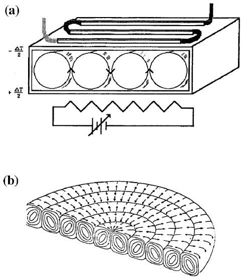
Figure 1. (a) A schematic picture of a Rayleigh-Bénard convection apparatus. Two horizontal flat plates of high thermal conductivity (typically made of copper or sapphire) are separated by a vertical height $d$ and the gap is filled with a fluid such as water. A spatially uniform and time-independent vertical temperature gradient is imposed on the fluid by heating the bottom plate to a fixed temperature $T_{\rm lower}=T+\triangle{T}/2$ (e.g., by a variable current flowing through resistors) and cooling the upper plate to a temperature $T_{\rm upper}=T-\triangle{T}/2$ where $T$ is the mean temperature of the fluid. The positive temperature difference $\triangle{T}$ across the fluid is the bifurcation parameter for driving the system from equilibrium. (b) Cross-section of curved convection rolls. For light directed vertically into the fluid and reflected off the bottom plate, the alternating warm and cold regions of convecting fluid act as diverging and converging lenses, allowing the spatial pattern to be visualized by shadowgraphy as alternating light and dark bands (see Fig. 2).

has become a central paradigm for experimental and theoretical research in large-aspect-ratio nonequilibrium physics. Convection does not quite involve the minimum number of components possible in a fluid experiment since there is a temperature field in addition to the usual velocity and pressure fields of the Navier-Stokes equations. But the presence of the temperature field has the important consequence of allowing a continuous bifurcation, from a uniform motionless conducting state to a state of finite-amplitude convection rolls in which warm fluid rises and cold fluid falls spatially over a characteristic wavelength that is basically twice the depth $d$ of the fluid, $\lambda_{c}\approx 2d$. Some other experimental advantages of Rayleigh-Bénard convection are the ease of building highly precise containers with static homogeneous boundaries, the ease of visualization throughout the interior of the fluid, the slow increase in complexity of the dynamics as the temperature gradient is increased, and the absence of a mean flow. As pointed out above, a drawback is the long time scale for transients to decay, a lower bound for which is given by the horizontal (lateral) thermal diffusion time.

A convection experiment can be described by a minimum of three dimensionless parameters [Bus78]. The most important is the Rayleigh number $R=\alpha gd^{3}\triangle{T}/\nu\kappa$ where $\alpha$ is the thermal-expansion coefficient of the fluid, $g$ is the acceleration of gravity (the source of buoyancy forces), $d$ is the depth of the fluid, $\triangle{T}$ is the vertical temperature difference across the plates, $\nu$ is the kinematic viscosity, and $\kappa$ is the thermal diffusivity. In a typical experiment or simulation, all of the parameters entering the Rayleigh number are fixed except the temperature difference $\triangle{T}$, and so the Rayleigh number is conveniently thought of as being proportional to the temperature difference across the plates. A linear stability analysis of the conducting fluid in a laterally infinite layer shows that convection begins when the Rayleigh number increases beyond a critical value $R_{c}=1707.76\cdots$, which corresponds to a temperature difference of a few degrees Celsius in room-temperature water experiments with fluid depths of a few millimeters. Since the bifurcation to convection is continuous, it is convenient to introduce a reduced Rayleigh number, $\epsilon=(R-R_{c})/R_{c}$ which is a small parameter near onset. Perturbative expansions in $\epsilon$ near onset lead to the amplitude equation formalism [CH93] which has made many successful quantitative predictions concerning pattern formation.

A second dimensionless parameter is the Prandtl number $\sigma=\nu/\kappa$, which is the ratio of the strengths of the two channels of dissipation. The Prandtl number influences the types of secondary bifurcations which convection rolls undergo at higher Rayleigh number, but weakly affects the dynamics sufficiently close to onset. It is a fluid property that is weakly dependent on temperature and is of order one for many gases. Different experimental values can be selected by using different fluids such as large-$\sigma$ oils, moderate-$\sigma$ gases, and low-$\sigma$ liquid mercury. A third dimensionless parameter is the aspect ratio $\Gamma=L/d$ (where $L$ is the largest lateral distance), which determines how weakly the lateral boundaries influence the dynamics. For this review, the aspect ratio is the interesting parameter since it provides a way to increase dynamical complexity. Computational scientists can simulate three-dimensional convection with periodic lateral boundary conditions in which case only the parameters $R$, $\sigma$, $\Gamma$, together with initial data, need to be specified. For experimentalists who require real walls to contain a fluid, other parameters must be considered such as the thermal boundary conditions on the lateral walls (which often have a thermal conductivity comparable to the fluid) and the shape of the container. Experimentally and theoretically, the influence of these other parameters on dynamics is not well understood although some experiments show that the choice of lateral boundary conditions can strongly influence the spatiotemporal dynamics [MAC91]. How this influence varies with increasing aspect ratio is a key question to resolve with future research.

The quantitative study of large-aspect-ratio dynamics began in 1978, with a pioneering Rayleigh-Bénard convection experiment by Guenter Ahlers and Robert Behringer who were then at AT&T Bell Laboratories [AB78]. These researchers studied the onset of convection in liquid helium at cryogenic temperatures of a few degrees Kelvin. Using convection cells with three different aspect ratios of about 2, 5, and 57, they made the remarkable and unexpected discovery that the Rayleigh number $R_{t}=R_{t}(\Gamma)$ at which turbulent or chaotic behavior was first observed (as the Rayleigh number was increased in small constant steps from below to above the onset of convection) decreased with increasing $\Gamma$, and seemed to approach the onset of convection itself, $R_{t}\to R_{c}$, as the aspect ratio became large. In fact, within experimental error the Ahlers-Behringer experiment for $\Gamma=57$ said that the onset of chaos coincided with the onset of convection, $R_{t}\approx R_{c}$. This last point was a particularly exciting development since it showed for the first time that a turbulent state existed in a parameter range that might be quantitatively amenable to perturbation theory (in the small parameter $\epsilon=(R-R_{c})/R_{c}\to 0^{+}$).

The discovery of chaos close to the onset of convection in a large aspect-ratio cell was a big surprise at the time and is still not well understood today, eighteen years later. The reason for the surprise was that a linear stability theory of periodic two-dimensional roll solutions of the Boussinesq equations in a laterally infinite container, had been developed over many years by Fritz Busse and collaborators [Bus78]. This theory predicted that stable time-independent periodic convection rolls should exist sufficiently close to onset, with the roll wavelengths lying in a known range that depends on both $R$ and $\sigma$ [SLB65]. This prediction had been qualitatively confirmed by prior experiments in smaller aspect ratio cells and was therefore expected to be more quantitatively correct in the limit of large aspect ratio, which approached the theoretical assumption of a laterally infinite container. Busse’s theory further predicted that, with increasing $R$, all periodic two-dimensional rolls eventually became unstable above some Rayleigh number $R_{u}=R_{u}(\sigma)$ although some rolls may first become unstable for values of $R$ smaller than $R_{u}$ depending on their wavelength. What happens for $R>R_{u}$ (all two-dimensional periodic rolls unstable) is a long-time nonlinear effect not predicted by a linear analysis: the unstable rolls could evolve into a new stationary pattern (e.g., consisting of curved convection rolls) or into a sustained time-dependent state. In any case, the linear stability theory together with prior experiments suggested that any time-dependent behavior, and certainly any chaotic behavior, would not be seen until the reduced Rayleigh number $\epsilon=(R-R_{c})/R_{c}$ was of order one, and this result should hold especially in the limit of large aspect ratio.

An irony of this pioneering experiment was that no visual information was available to indicate the spatial patterns of the convecting fluid. Ahlers and Behringer had obtained their conclusions by analyzing time series of the Nusselt number, which is a dimensionless scalar measure of the total heat transported from the bottom plate to the top plate of the convection experiment. Not until 1985, with an innovative high-pressure gas experiment of Pocheau, Croquette, and Le Gal [PCL85], did researchers succeed for the first time in visualizing large-aspect-ratio convection patterns. The details of that experiment largely exceeded the imagination of those who had tried to guess the mechanism of the time dependence in the Ahlers-Behringer experiment. Some of these details are illustrated in Fig. 2, which is taken from a recent and more refined version of a pressurized gas convection experiment [MBCA96].

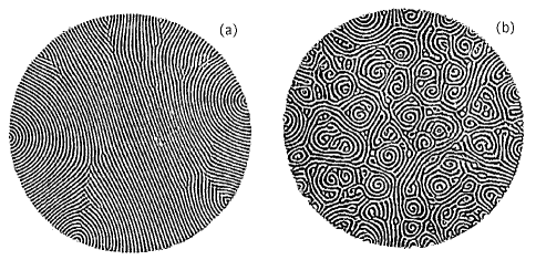
Figure 2. Two instantaneous Rayleigh-Bénard convection patterns from different spatiotemporal chaotic states, in a $\Gamma=74.6$ cylindrical convection cell [MBCA96]. The patterns were observed by shadowgraphy; the white areas correspond to cool gas descending into the plane of the figure and the dark areas correspond to warm gas rising out of the plane of the figure. Pattern (a) corresponds to a fixed reduced Rayleigh number $\epsilon=0.243$ while pattern (b), a spiral-defect chaos state, is more strongly driven with $\epsilon=0.894$. These chaotic states occur in a range of reduced Rayleigh number $\epsilon<\epsilon_{u}\approx 2$ for which theory predicts the existence of stable periodic infinite two-dimensional rolls. The convecting fluid is gaseous carbon dioxide at a mean temperature of about $30^{\circ}\,\rm C$, with Prandtl number $\sigma=0.94$, and under a pressure of $p=33\,\rm bar$. The local periodicity of the convection rolls, disrupted by defects, is a general feature of many large spatiotemporal chaotic states.

Patterns (a) and (b) immediately suggest (as did the earlier experiment of Pocheau et al) why the Busse stability analysis did not apply to the Ahlers-Behringer experiment, although both for different reasons. Fig. 2(a) shows that even for this large aspect ratio, the lateral boundaries can have a strong effect on the geometry of the convection rolls, which have a substantial curvature and so are three-dimensional over much of the interior of the convection cell. This curvature can be understood qualitatively as a consequence of the cylindrical geometry, of the empirical fact that convection rolls tend to be perpendicular to the side walls for certain lateral thermal boundary conditions, and of the fact that near onset, the rolls oscillate spatially within a narrow range of wavelengths centered on the critical wavelength $\lambda_{c}\approx 2d$. Further from onset, but still below the Rayleigh number for which all two-dimensional infinite periodic rolls are unstable, Fig. 2(b) shows that the Busse stability analysis can fail because the basic pattern can be so disordered that there are no substantial regions of straight rolls. Measurements suggest that the chaotic state in the interior of Fig. 2(b) does not depend on the shape or size of the convection cell [MBCA96] and thus this state (unlike Fig. 2(a)) is a good candidate for studying the thermodynamic limit of infinite system size. Despite the intricate time-dependent structure of both patterns, they still consist of locally periodic rolls, with a distribution of local wavelengths that is almost entirely stable according to Busse’s linear stability analysis [HFG85, MBCA93].

Since the above 1978 and 1985 experiments, many other experiments, simulations, and analytical calculations—on convection and on other systems—have shown that large homogeneous sustained nonequilibrium systems with spatiotemporal chaos have various features in common that we briefly summarize [CH93]:

1. Sufficiently large systems typically have chaotic solutions and the chaos can occur close to the primary instability from a uniform state as the system size increases. Bigger systems seem to be more susceptible to chaos although a precise statement of this fact has yet to be made.

2. The spatiotemporal dynamics is often associated with defects (regions where a local periodicity can not be defined [CH93, Section V.B, page 898]), whose dynamics seem to determine both the spatial and temporal disorder (but not the fractal dimension as discussed in Section 4 [OEG96]). These defects are evident in Fig. 2(a), which has focus singularities, dislocations, disclinations and grain boundaries, and in Fig. 2(b) which has in addition spiral and target defects. The time evolutions of these states show that the defects can nucleate, annihilate, move, and interact with other defects and with lateral boundaries. Over the past fifteen years, researchers have studied the dynamics of isolated defects and of isolated pairs of defects, with the hope (not yet realized) that insights of few-defect dynamics might apply to many-defect states such as Fig. 2(b). A good example of this approach is the recent theoretical paper by Cross and Tu [CT95] on the spiral-defect chaos state of Fig. 2(b).

3. From both experimental and computational studies of large-aspect-ratio systems, there seem to be only a few bifurcations that lead from the uniform state to spatiotemporal chaos as the system is driven further from equilibrium. After the onset of spatiotemporal chaos, further distinguishable bifurcations are rarely observed, although this may reflect our present inability to identify such bifurcations theoretically. These qualitative observations suggest, somewhat paradoxically, that the thermodynamic limit may be easier to understand than low-dimensional chaos since there exist only a few phases in that limit [SPS⁺92]. For small-aspect-ratio low-dimensional models, there can be an infinity of bifurcations over a finite parameter interval, e.g., for the logistic map or for the Lorenz equations [Str94].

4. There have been few examples discovered or studied in which nontrivial critical exponents occur at a continuous bifurcation in a large-aspect-ratio system. One example is the bifurcation of a chaotic to uniform (laminar) state via spatiotemporal intermittency, which was predicted to lie in the universality class of directed percolation [CH93, Page 954]. Experiments and simulations did not confirm this prediction although some details need to be studied further. A more recent example (discussed in Section 4 in another context) is a study by Miller and Huse of a two-dimensional deterministic spatiotemporal chaotic nonequilibrium lattice that undergoes an Ising-like phase transition as a coupling constant is varied [MH93]. These authors used analytical and numerical calculations to argue that this deterministic nonequilibrium model should behave exactly like the equilibrium two-dimensional Ising model at long wavelengths (i.e., near the Ising phase transition). Some doubt was recently cast on this conclusion by ambitious numerical simulations of the Miller-Huse model by Marcq et al [MCM96], who found evidence for critical exponents that are close to, but distinctly different than the Ising values. This discrepancy is important to resolve since it would help to identify when equilibrium statistical mechanics might apply to sustained nonequilibrium systems. A related area of future research would be to understand the possible relevance of probabilistic (as opposed to deterministic) nonequilibrium models for understanding deterministic dynamics. There has been considerable research concerning the critical properties of probabilistic models, which show a wider variety of universality classes than those found in equilibrium systems [SZ95].

We finish this section by coming back to one of the questions raised by the Ahlers and Behringer experiment: is it true that the onset of chaos approaches the onset of convection in the limit of infinite aspect ratio: $R_{t}\to R_{c}$ as $\Gamma\to\infty$? This seems to be a delicate question that will be difficult to settle by experiment or by simulations, because of the diverging transient time as $\Gamma$ becomes large. To some extent, interest in this question has been preempted by more recent theory and new experiments which show that, for a convection cell rotating at a constant angular frequency $\Omega$, the onset of chaos should rigorously coincide with the onset of convection above a critical rotation speed $\Omega_{c}$. This system thus seems to be particularly attractive for studying the thermodynamic limit since analytical progress should be possible near onset [CMT94].

4. Characteristic Length Scales of Spatiotemporal Chaos

From the discussion of the previous section, we see that a key challenge for understanding how complexity scales with size, for large homogeneous sustained nonequilibrium systems, is to find ways to characterize the spatiotemporal disorder that is commonly observed. This problem is difficult physically and mathematically. The lack of conservation laws, detailed balance, and free-energy-like functionals has hindered the development of a basic theory of sustained nonequilibrium systems that could indicate appropriate quantities to measure, e.g., ones perhaps analogous to scalar macroscopic equilibrium parameters such as the temperature or chemical potential. The nonperiodicity of spatiotemporal chaos makes the problem of characterization mathematically open-ended since there is an infinity of ways to characterize slippery concepts like “disordered”, “random” [Knu81, Section 3.5] and “complex” [Zur90]. For example, random fields can be described incompletely by an infinity of $n$-point correlation functions (of which only the $2$-point function is routinely computed), and a high-dimensional strange attractor (perhaps the source of the random fields) can be described incompletely by the infinity of multifractal dimensions $D_{q}$ [Ott93] (of which only one value, the correlation dimension $D_{2}$, is routinely calculated). Further, many proposed mathematical definitions for “random” are not computable from finite amounts of imprecise data and, even when they are, they have not been compared with each other in a systematic statistical way. Given these difficulties, it is better to look carefully at specific experimental and computational results such as Fig. 2 for guidance in posing theoretical questions. As an example, Fig. 2(b) shows spirals of a certain characteristic average width and this width turns out to vary with Rayleigh number $R$ and with Prandtl number $\sigma$. For this particular experiment, one could then try to predict how this width varies with parameters [CT95].

In this section, this more modest approach is pursued and we consider some recent efforts to answer a basic question suggested by experiments and simulations: what length scales are associated with homogeneous spatiotemporal chaos? If various length scales are identified, one can further ask how they vary with parameters and with each other. The calculations discussed below show that there are at least two independent length scales associated with homogeneous spatiotemporal chaos. One length scale, the two-point correlation length $\xi_{2}$, is determined by the time-averaged spatial disorder as measured by the two-point (or the mutual information [OEG96]) correlation function of a field. The second length scale, the dimension correlation length $\xi_{\delta}$, arises from the extensivity of fractal dimensions in phase space. We discuss these two length scales in turn and then demonstrate that they are independent by studying a nonequilibrium model for which the length $\xi_{2}$ diverges while the length $\xi_{\delta}$ remains finite as a parameter is varied [OEG96]. Some implications of the fact that these length scales are independent from one another are then discussed.

4.1. What does a two-point correlation length $\xi_{2}$ mean?

The two-point correlation function of a random field has a long tradition of application in fluid dynamics and in condensed matter physics because of the ease with which it can be computed and because theory is sometimes able to predict some of its features. However, its meaning in a spatiotemporal context is not so clear as we now discuss. To introduce some notation and definitions, let us consider a nonperiodic spatiotemporal scalar field $u(t,x)$ which is assumed for simplicity to be one-dimensional with zero mean. (The field $u(t,x)$ could be the temperature field fluctuations $T(t,x,y_{0},z_{0})-\langle T\rangle$ measured along some $x$-coordinate in a Bénard convection cell.) For spatial coordinates $x^{\prime}$ and $x$, the two-point correlation function $C_{2}(x^{\prime},x)$ is defined by

(4.1) $$C_{2}(x^{\prime},x)=\left\langle u(t,x^{\prime})u(t,x)\right\rangle,$$

where the brackets $\langle\cdots\rangle$ denote averaging over the time variable $t$ (and perhaps also over realizations calculated independently on different processors of a parallel computer [Ego94]). For the homogeneous systems that we assume, $C_{2}=C_{2}(|x^{\prime}-x|)$ is a function of only the magnitude of the difference between the spatial positions. In many (but not all) cases, the two-point correlation function asymptotically decays exponentially for a sufficiently large spatial separation,

(4.2) $$C_{2}(|x^{\prime}-x|)\to\exp(-|x^{\prime}-x|/\xi_{2}),\qquad\mbox{as $|x^{\prime}-x|\to\infty$}.$$

which defines the two-point correlation length $\xi_{2}$. Fig. 4 of Ref. [OEG96] illustrates this exponential decay for the two-dimensional Miller-Huse model [MH93], from which the length $\xi_{2}$ can be extracted from a log-linear plot.

An important point to appreciate in the definition Eq. (4.1) is that the definition of $C_{2}$ is only weakly dependent on time correlations of spatial fields. If one considers Eq. (4.1) as averaging over various snapshots at different times $t$ of the product $u(t,x^{\prime})u(t,x)$, then the order of the snapshots does not matter in the summation. It is then unclear how the spatial disorder measured by $\xi_{2}$ relates to the deterministic dynamics that generates the disorder. As an example, meteorologists since the 1950’s have measured two-point correlation functions of the earth’s weather patterns, e.g., of the varying heights on a constant pressure surface [Bue58, Figure 5, page 507]. (The author is indebted to Edward Lorenz for this reference.) The correlations measured from a specific point do not fall off exponentially rapidly with increasing distance but do fall off substantially over a length scale of about $1500\,\rm km$, which we take as an estimate of the two-point correlation length $\xi_{2}$. If the weather at two different points is dynamically (not just spatially) uncorrelated when the points are further apart than about the distance $\xi_{2}$, then the earth’s weather system might be understood as consisting of weakly interacting, statistically independent subsystems of size $\xi_{2}$. The number $N$ of such subsystems can be estimated from the ratio of the earth’s surface area to to the area of an approximately circular subsystem:

(4.3) $$N\approx\frac{4\pi R_{e}^{2}}{\pi\xi_{2}^{2}}\approx\frac{4\pi 6400^{2}}{\pi 1500^{2}}\approx 70,$$

where we have used the value $R_{e}=6400\,\rm km$ for the radius of the earth. Since each subsystem has its own complex internal dynamics with many degrees of freedom, Eq. (4.3) would provide a lower bound to the fractal dimension of the earth’s weather. The value of $70$ is consistent with the failure of time-series-based algorithms [ABT93] to estimate the fractal dimension of the weather since these algorithms fail to converge for fractal dimensions larger than about five [Poo89, Lor91].

Similarly, a recent cardiology experiment has provided some of the first spatiotemporal voltage measurements on the surface of a pig’s heart that was ingeniously kept in sustained fibrillation for many minutes [BJG⁺93]. From this data, a two-point correlation function was calculated which, although it did not decay exponentially, did fall off sufficiently rapidly so as to suggest a two-point correlation length $\xi_{2}\approx 6\,\rm mm$. From the average radius of the pig heart $R_{\rm pig}\approx 25\,\rm mm$, the arguments leading to Eq. (4.3) can be used to estimate the number $N$ of independent subsystems on the surface of the fibrillating heart, which turns out to be $N\approx 70$. (The appearance of the number $70$ in both estimates is purely coincidental and has no known religious significance.) As a lower bound to the fractal dimension of the heart, the value 70 is consistent with the inability of researchers to detect low-dimensional dynamics in ventricular fibrillation by traditional time series methods [WKP⁺95].

Is it reasonable to expect the two-point correlation length $\xi_{2}$ to provide dynamical information as suggested above, which could cut the Gordian knot of not being able to calculate large fractal dimensions from data? A simple argument suggests that $\xi_{2}$ and $D$ are generally independent quantities. One can disorder a phonograph record by drilling holes into it in such a way so as to impose any desired correlation length $\xi_{2}$. By then rotating the phonograph record rigidly with an angular frequency $\omega(t)$ derived from some $D$-dimensional dynamical system, time series of any desired fractal dimension can be created for any specified correlation length $\xi_{2}$. Fig. 2 and related time evolutions suggest, however, that such phonograph dynamics is not representative of spatiotemporal chaotic states which typically involve the non-rigid motion of defects. A quantitative exploration of a relation between the fractal dimension $D$ and length $\xi_{2}$ might then be insightful.

4.2. The Dimension Correlation Length $\xi_{\delta}$

A possibly different length scale associated with spatiotemporal chaos can be found by thinking about attractors in phase space, rather than about the disorder of fields such as $u(t,x)$. As David Ruelle first pointed out in 1982 [Rue82], widely separated subsystems of a turbulent flow should be weakly correlated in which case the spectrum of Lyapunov exponents $\lambda_{i}$ for the entire system should be the union of exponents associated with each of the non-interacting subsystems. This implies that the spectrum should be intensive in the sense that $\lambda_{i}=f(i/V)$ is a function only of an intensive index $i/V$ where $V$ is the volume of the system. This further implies (via Eq. (4.4) below) that the fractal dimension $D$ of an attractor should be extensive, i.e, $D\propto V$, for sufficiently large system size $L$, in which case we say that the dynamical system has extensive chaos. The extensivity of $D$ was first demonstrated numerically by Paul Manneville in 1985 for chaotic solutions of a one-dimensional partial differential equation, the Kuramoto-Sivashinsky equation [Man85].

Extensivity of $D$ has since been established numerically in other one- and two-dimensional mathematical models (see Fig. 5 below) and in fact has been proposed by Cross and Hohenberg to be the essential defining feature of spatiotemporal chaos [CH93, Page 945]. This definition presently has the serious drawback of not being computable with experimental data. Only one numerical method is known for calculating fractal dimensions of high-dimensional dynamical systems which is the Kaplan-Yorke formula for the Lyapunov dimension $D_{\mathcal{L}}$ in terms of the spectrum of Lyapunov exponents:

(4.4) $$D_{\mathcal{L}}=K+\frac{1}{|\lambda_{K+1}|}\sum_{i=1}^{K}\lambda_{i},$$

where the integer $K$ is the largest integer such that the sum of the first $K$ Lyapunov exponents is nonnegative. The formula for $D_{\mathcal{L}}$ has been proved to be equal to the information dimension $D_{1}$ in some cases [Ott93], but it is not known whether this equality holds for extensively chaotic systems. With present algorithms based on time series [ABT93], only the first few largest exponents can be calculated reliably, which usually are not enough to determine the integer $K$ in Eq. (4.4). If dynamical equations are known explicitly (so that the equations can be linearized analytically around some given nonlinear solution), then all the Lyapunov exponents can be calculated numerically by studying directly the exponential growth of hypervolumes of infinitesimal simplices in the tangent space of some given nonlinear orbit [PC89]. The computational effort to find enough exponents to use Eq. (4.4) (all the positive and enough negative ones) grows only algebraically with the dimension $D_{\mathcal{L}}$, as opposed to exponentially with $D_{\mathcal{L}}$ for algorithms based on time series. Even with this algebraic growth, most calculations of $D_{\mathcal{L}}$ are computationally intense and only recently, with the increasing availability of parallel computers, have researchers been able to calculate the Lyapunov spectrum and dimension of many one- and two-dimensional extensively chaotic mathematical models.

Since the dimension $D_{\mathcal{L}}$ grows in proportion to the system volume $V$ for large enough $V$, the dimension is itself not an interesting quantity since it merely indicates the size of the system. More useful is to define an intensive Lyapunov dimension density $\delta$:

(4.5) $$\delta=\lim_{V\to\infty}D_{\mathcal{L}}/V,$$

which can be thought of as the number of active degrees of freedom per unit volume. Since the dimension density has physical units of inverse volume, Cross and Hohenberg [CH93] suggest going one step further by defining a dimension correlation length $\xi_{\delta}$:

(4.6) $$\xi_{\delta}=\delta^{-1/d},$$

where $d$ is the dimensionality of the system (e.g., $d=2$ for a large-aspect-ratio convection experiment). This length can then be readily compared with other lengths such as the critical wavelength $\lambda_{c}$, the two-point correlation length $\xi_{2}$, and the largest lateral system size $L$.

Two examples may help to interpret the meaning of $\xi_{\delta}$, which may be thought of as the radius of a volume that contains one degree of freedom. If a one-dimensional system of length $L$ has a stable limit cycle as the length $L$ is varied (e.g., a stable plane wave), then the dimension $D=1$ (any limit cycle has dimension one), the dimension density $\delta=1/L$ is a small number that vanishes with increasing $L$, and $\xi_{\delta}=1/\delta=L$ is a big length equal to the size of the system. An opposite extreme would be a one-dimensional coupled map lattice with $L$ sites, with each site containing a chaotic tent map of dimension $D=1$. In the limit of zero coupling, the dimension $D\to L$, $\delta\to 1$, and $\xi_{\delta}\to 1$ approaches the distance between neighboring sites and is small compared to the system size $L$. It would be interesting to determine the values of $\xi_{\delta}$ for the two chaotic states of Fig. 2, e.g., from simulations with two-dimensional Generalized Swift-Hohenberg equations [XG95] or indirectly from experimental data by using the extensive scaling of the Karhunen-Loève decomposition [ZG96]. A reasonable conjecture is that Fig. 2(b) will have a smaller value of $\xi_{\delta}$ than Fig. 2(a).

4.3. A Comparison of Two-Point and Dimension Correlation Lengths

Are the two correlation lengths  $\xi_{2}$ and $\xi_{\delta}$ related for homogeneous spatiotemporal chaos, i.e., does average spatial disorder determine dynamical complexity? It is unlikely that they would be equal to each other but a falsifiable hypothesis is that they are proportional to one another, $\xi_{2}\propto\xi_{\delta}$, in which case they should be considered to be equivalent. One way to test this hypothesis is to find a mathematical model of a sustained nonequilibrium system for which one of these quantities varies strongly with parameters and then to compare one with the other. A hint of how to find such a model comes from the theory of critical phenomena, which tells us that the correlation length $\xi_{2}$ diverges to infinity near a second-order phase transition of an equilibrium system [LL80, Section 148]. This observation poses several difficult physics questions: what is meant by a phase transition in an infinite nonequilibrium system? Do any examples exist and, if so, do nonequilibrium phase transitions have critical properties?

Two recent candidates for such models have been recently studied by my group at Duke, the one-dimensional complex Ginzburg-Landau (CGL) equation [EG94, EG95, Ego94] and the two-dimensional Miller-Huse model [OEG96]. For simplicity, I briefly review some results for the Miller-Huse model, which more clearly succeed in falsifying the above hypothesis, and which are also interesting in their own right [OEG96]. The discussion will also help to illustrate some of the ideas discussed in previous sections such as how a system approaches extensive behavior and how the length $\xi_{\delta}$ is calculated.

The Miller-Huse model is a clever deterministic nonequilibrium version of the famous two-dimensional Ising model [LL80], which itself models the continuous onset of ferromagnetic order for discrete magnetic spins (i.e., when the spins all align in the same direction), as the temperature is decreased from the paramagnetic (unmagnetized) phase. The model is a coupled map lattice (CML) in which space and time are discretized and the lattice variables have continuous real values. (There is no meaningful continuum limit of this model as the lattice spacing and time step go to zero, as would be the case for the numerical discretization of a partial differential equation.) On a finite two-dimensional $L\times L$ square lattice with periodic boundary conditions, a piecewise-linear one-dimensional chaotic map $y_{i+1}=\phi(y_{i})$ is placed on each of the $L^{2}$ lattice sites. The output of each map is then coupled to its nearest neighbor values by a simple linear diffusive coupling with strength $g$. The model is not intended to correspond closely to any physical system but, in the spirit of the Ising model and of critical phenomena, some details at long wavelengths are expected to be independent of the lattice and of the lattice map, and so might correspond to actual physical systems. That a phase transition might occur can be understood as a competition between local chaos, which generates disorder, and diffusion, which tends to damp disorder.

The CML is defined mathematically in the following way. Let us denote by $y^{t}_{i}\in[-1,1]$ the variable at spatial site $i$ at integer time $t$ (with $t=0$, $1$, $\cdots$), and then define the following rule for updating each lattice variable synchronously to time $t+1$ [MH93]:

(4.7) $$y_{i}^{t+1}=\phi(y_{i}^{t})+g\sum_{j(i)}\left(\phi(y_{j}^{t})-\phi(y_{i}^{t})\right),$$

where the parameter $g$ is the spatial coupling constant and where the sum goes over the four indices $j(i)$ that are nearest neighbors to site $i$. The function $\phi$ defining the local map is given by

(4.8) $$\phi(y)=\left\{\begin{array}[]{ccrcccr}-2-3y&\mbox{for}&\mbox{$-1$\ }&\leq&y&\leq&-1/3,\\ 3y&\mbox{for}&-1/3&\leq&y&\leq&1/3,\\ 2-3y&\mbox{for}&1/3&\leq&y&\leq&\mbox{$1$,\ }\end{array}\right.$$

and is shown in Fig. 3, together with a representative time series of its chaotic dynamics.

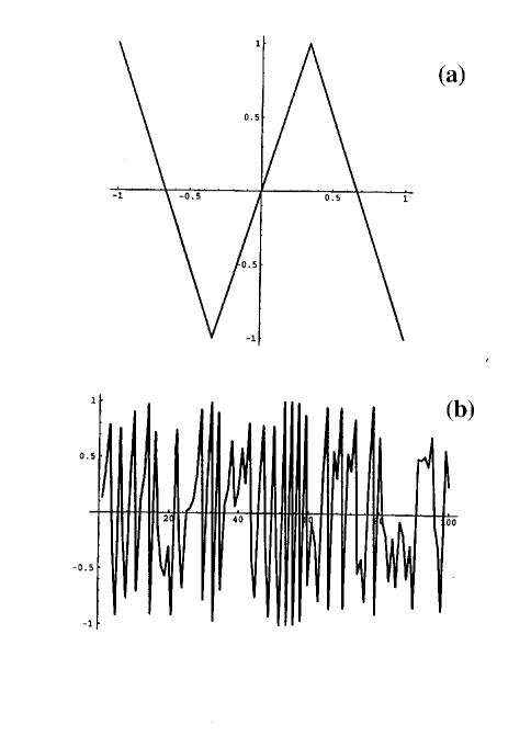
Figure 3. (a) Plot of the odd Miller-Huse map $y_{i+1}=\phi(y_{i})$, Eq. (4.8) of the interval $[-1,1]$ into itself. The map has a slope of constant magnitude 3 everywhere and is chaotic for nearly all initial conditions in the interval $[-1,1]$. (b) Time series $y_{i}$ versus $i$ for 100 iterations of the Miller-Huse map, illustrating its chaotic behavior.

It maps the interval $[-1,1]$ into itself and is chaotic since the map has a slope of constant magnitude equal to 3 which is everywhere greater than one. A crucial insight of Miller and Huse was to choose the local map Eq. (4.8) to have odd parity, $\phi(-y)=-\phi(y)$, which turns out to be necessary (but not sufficient) to allow an Ising-like phase transition. Positive and negative values of lattice variables then correspond to the up-spin and down-spin magnetic variables of the Ising model.

As a function of the lattice coupling parameter $g$, the qualitative behavior of this CML can be described as follows. If one initializes each lattice variable $y^{0}_{i}$ inside the interval $[-1,1]$ and provided $g$ is smaller than $1/4$, the dynamics will be bounded forever. For small values of $g$, the dynamics settle down after some transient into a spatiotemporal chaotic state consisting visually of small domains of sites that all have negative or positive values together; these regions of similar sign are called “droplets” by analogy to the clusters of up- and down-spins found in the Ising model (Fig. 4).

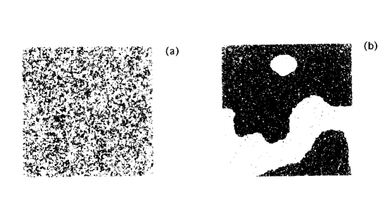
Figure 4. Onset of long-range spatial order in the two-dimensional Miller-Huse CML on a periodic $128\times 128$ square lattice, as the coupling constant $g$ is increased from below to above the phase transition point at $g_{c}=0.205$. Sites with positive and negative lattice values are colored red and green respectively. (a) Instantaneous lattice values for $g=0.190$, for which the two-point correlation length $\xi_{2}=3$ is comparable to the lattice spacing. (b) Instantaneous lattice values for $g=0.235$ for which $\xi_{2}$ is comparable to the size of the system. The two green droplets eventually annihilate leaving a homogeneous “ferromagnetic” red state.

These small fluctuating droplets corresponds to a high-temperature disordered paramagnetic phase. As $g$ is increased towards the critical value $g_{c}=0.205$, the dynamics remain chaotic and the droplets grow in size. Correspondingly, the correlation length $\xi_{2}$ of the field values $y^{t}_{i}$ starts to increase until it becomes of order the system size at the critical value $g_{c}$. For still larger values of $g$, one finds just one or two droplets spanning the entire lattice, corresponding to a low-temperature ferromagnetic, ordered phase. The idea is then to compare the lengths $\xi_{2}$ and $\xi_{\delta}$ across the nonequilibrium transition point of $g=0.205$ as $\xi_{2}$ diverges to infinity.

For coupling constant $g=0.199$, Fig. 5 shows that the Miller-Huse CML is, in fact, extensively chaotic as the lattice area (total number of lattice sites $N$) is increased.

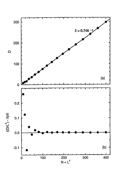
Figure 5. Lyapunov fractal dimension $D$ versus the area of the lattice $N=L^{2}$ for the periodic Miller-Huse CML Eq. (4.8) and for coupling constant $g=0.199$. The dimension $D$ was calculated from the Kaplan-Yorke formula Eq. (4.4) by iterating the CML for  $T=50,000$ iterations after transients died out. (a) The dimension grows linearly and extensively with lattice area for $N>100$. The slope of this curve for large $N$ gives a dimension density $\delta=0.746$, corresponding to a dimension correlation length $\xi_{\delta}=\delta^{-1/2}=1.16$. (b) The normalized deviation $(D/N-\delta)/\delta$, of the dimension density $\delta$ from the value $D/N$, illustrates the rapid approach to extensive scaling for small systems sizes $L>9$.

For small $N$, the Lyapunov dimension $D_{\mathcal{L}}$ behaves irregularly, which corresponds to the sensitive dependence of low-dimensional dynamics on parameter changes. For lattices sizes $L$ larger than about 9, the extensive regime begins and $D_{\mathcal{L}}$ grows linearly with $N$. The dimension density $\delta=0.746$ is obtained from a least-squares fit of the linear part of the curve and this value corresponds to a dimension correlation length of $\xi_{\delta}=\delta^{-1/d}=\delta^{-1/2}=1.16$ which is comparable to one lattice spacing. Fig. 5(b) shows that the onset of extensive behavior is not abrupt. The deviation from extensivity decays rapidly and non-monotonically.

Fig. 6 is the most important figure in this paper and shows how the two lengths, $\xi_{2}$ and $\xi_{\delta}$, vary in the vicinity of the Miller-Huse nonequilibrium phase transition at $g_{c}=0.205$.

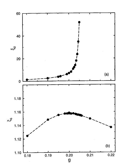
Figure 6. Variation of (a) the two-point correlation length $\xi_{2}$ and (b) the dimension correlation length $\xi_{\delta}$ with the coupling constant $g$ for the Miller-Huse CML on a square periodic lattice. The length $\xi_{2}\propto(g-g_{c})^{-\nu}$ diverges with an exponent $\nu\approx 1$ [MCM96] near the critical value $g_{c}=0.205$ while the length $\xi_{\delta}$ is bounded and varies smoothly, attaining a local maximum at a value $g=0.200$ that is distinctly less than $g_{c}$. Lattice sizes of up to $L=1024$ were used to calculate these lengths, with integration times of up to $T=3\times 10^{5}$.

As is the case with the Ising model, the two-point correlation length diverges at the critical value $g_{c}$, $\xi_{2}\propto(g-g_{c})^{-\nu}$, with critical exponent $\nu\approx 1$ in accord with the arguments of Miller and Huse [MCM96]. In contrast, Fig. 6(b) shows that $\xi_{\delta}$ over the same range of $g$ is bounded and varies smoothly over the small range of 1.12 to 1.16, attaining a local maximum at the value $g=0.200$ which is distinctly less than the value $g_{c}$ at which the transition occurs.

Despite the dramatic ordering of lattice variables with increasing $g$ as depicted in Fig. 4, we conclude that there is no relation between the average spatial disorder (as measured by the diverging two-point correlation length $\xi_{2}$) and the dynamical complexity of the corresponding strange attractor (as measured by the intensive dimension correlation length $\xi_{\delta}$). At least two length scales, and likely an infinity of lengths scales, are needed to characterize homogeneous spatiotemporal chaos. An unfortunate corollary is that the length $\xi_{2}$ can not be used to estimate the dimension density $\xi_{\delta}$ and hence the fractal dimensions of complex dynamical systems like the weather and the heart, as originally suggested by the heuristic arguments associated with (4.3).

Other calculations confirm these conclusions. Thus calculations for different system sizes $L$ of a one-dimensional partial differential equation, the complex Ginzburg-Landau (CGL) equation, show similarly that over a certain parameter range, the length $\xi_{2}$ can grow rapidly to large values while the length $\xi_{\delta}$ remains moderate and nearly constant [EG95, Ego94]. Calculations on a certain CML [BGHJ92] have shown that systems with generic algebraic decay of spatial correlations, for which the length $\xi_{2}$ is effectively infinite over a continuous range of parameters, can still be extensively chaotic, with a finite dimension correlation length $\xi_{\delta}$ [OEG97]. An interesting implication of these recent calculations is that $\xi_{\delta}$ always seems of moderate size, often comparable to the critical wavelength $\lambda_{c}$ of a pattern-forming instability and small compared to the two-point correlation length $\xi_{\delta}$. This suggests that many large-aspect-ratio experiments such as those shown in Fig. 2 are already in the extensively chaotic regime and can be used to test future theoretical work on extensive chaos.

These results present two interesting theoretical puzzles. One is to discover what mathematics and physics determines the magnitude of the length $\xi_{\delta}$. For the Miller-Huse CML, the value $\xi_{\delta}\approx 1$ says that the dynamics of each lattice map $\phi(y)$ is effectively independent of all others, even though the diffusive coupling leads to the onset of long range order as measured by $\xi_{2}$. This is somewhat plausible since there is a strong source of local chaos even in the absence of coupling between neighbors. The more mysterious situation is for systems with continuous spatial variables such as the CGL equation and for the convecting fluid in Fig. 2. In these cases, there is no chaos except in the presence of spatial coupling; sufficiently small isolated subsystems have either stationary or periodic nontransient dynamics.

The second theoretical puzzle is whether there is some way to estimate the dimension correlation length $\xi_{\delta}$ directly from finite amounts of imprecise experimental data. The calculations described above for the Miller-Huse CML used a brute-force computationally-intense method that first required calculating the Lyapunov fractal dimension of the entire system from known dynamical equations for several different volumes, and then extracting the length $\xi_{\delta}$ from the extensive scaling. This is utterly impractical for spatiotemporal data of the sort represented in Fig. 2 since there is no known way of calculating many Lyapunov exponents from time series recorded from high-dimensional systems. Instead, one might hope to exploit the fact that $\xi_{\delta}$ is an intensive quantity and so might depend only on information localized to some region of space.

There have been two recent attempts to estimate the value of $\xi_{\delta}$ from time series by generalizations of the Procaccia-Grassberger algorithm [Ott93] for low-dimensional systems [Tsi93, BHM93] but these efforts lack a rigorous justification and their numerical convergence is not convincing. More recently, Scott Zoldi and the author have proposed using a variation of the Karhunen-Lòeve decomposition (KLD) [Pre88], in which the KLD is applied to data in concentric volumes of increasing radius and then the KLD eigenvalues from these different calculations are combined to provide an estimate of an intensive correlation length $\xi_{\rm KLD}$ which has properties similar to the dimension correlation length $\xi_{\delta}$ [ZG96]. While this approach can not quantitatively predict the value of $\xi_{\delta}$, calculations for the Miller-Huse model show that the length $\xi_{\rm KLD}$ behaves qualitatively like $\xi_{\delta}$ as the coupling $g$ is varied, and so might serve the purpose of an easily calculated, localized order parameter for characterizing large, weakly inhomogeneous, spatiotemporal chaotic systems.

5. Conclusions

This survey article has discussed recent and ongoing efforts to understand how one particular mechanism—increase of system size—affects the complexity of nontransient homogeneous sustained nonequilibrium systems. Perhaps the single most important idea from this discussion is that of extensive chaos: for sufficiently large homogeneous chaotic systems, the fractal dimension $D$ (effective number of degrees of freedom) becomes proportional to the volume $V$ of the system as illustrated in Fig. 5. This mathematical statement can be interpreted physically as saying that big homogeneous systems become complex in a simple way with increasing size, by replicating weakly-interacting and statistically similar subsystems of some characteristic size that we have defined as the dimension correlation length $\xi_{\delta}$. Another interpretation of extensive chaos is that there are no interesting collective effects with growing size, as might be expected if small dynamical units somehow bind themselves into a larger effective unit with fewer total degrees of freedom. Collective effects would possibly appear as a proportionality $D\propto L^{\alpha}$ (where $L$ is the system size), with an exponent $\alpha$ that is not the dimensionality $d$ of the system.

Extensive chaos is important because it shifts attention away from characterizing a system by global quantities (e.g., by its fractal dimension), towards understanding the properties of a subsystem and how different subsystems interact. Research along these lines for sustained nonequilibrium systems is still only in its infancy [Zal89, BC92, MH93, EG95, CH95, OEG96, DHBE96] but should blossom in the near future if for no other reason that computer power continues to increase steadily, which will allow a wider variety of physical problems to be simulated and studied mathematically, and which will permit further quantitative comparisons between theory and experiment.

Besides surveying recent progress in theory and experiment, this review has also tried to point out interesting open questions. I conclude this paper by summarizing some of these questions, with the hope of stimulating further research:

1. A theme throughout this paper was that big homogeneous chaotic systems can be considered as a gas of weakly interacting subsystems. It would be insightful to find some way to demonstrate this idea directly, rather than indirectly by the extensive scaling of the fractal dimension. One idea would be to study how localized short-lived infinitesimal perturbations propagate in spatiotemporal chaotic systems. Do they die off substantially on the length scale of $\xi_{\delta}$?

2. Can the idea of a subsystem provide a way to quantify the dynamics of inhomogeneous sustained nonequilibrium systems, at least for the simplified case of parameter values that are slowly varying in space? If a spatially dependent parameter $p(x)$ varies on a length scale large compared to $\xi_{\delta}$, then one can speculate that a subsystem centered at position $x_{0}$ would, over a certain range of length and time scales, be similar to a subsystem of an infinite homogeneous dynamical system whose spatially uniform parameter value corresponds to the value $p_{0}=p(x_{0})$. This idea was recently confirmed for a Miller-Huse model with a spatially varying coupling constant $g$, using a correlation length based on the extensivity of the Karhunen-Lòeve decomposition [ZG96].

3. The Navier-Stokes equations can be considered as arising from a long-wavelength, long-time-scale averaging of molecular dynamics. Fig. 2(b) suggests an analogous reduction: over length scales large compared to the dimension correlation length $\xi_{\delta}$ (the size of the spirals in this figure?), can the intricate local dynamics be replaced by a simple hydrodynamic-like equation, perhaps with a Gaussian uncorrelated noise source arising from the local chaos? This has been successfully done in two cases, for the one-dimensional Kuramoto-Sivashinsky equation [CH95] and for a one-dimensional CML with a conserved quantity [BC92]. However, there are no principles known for deriving such equations or even for determining whether such equations exist.

4. Are intensive quantities like $\xi_{\delta}$ local quantities that depend only on information in a finite region of space? If so, are there time-series based algorithms that can estimate these intensive quantities, without first calculating an extensive quantity? The calculations of Ref. [ZG96] suggests that this should be possible but more work is needed.

5. What determines the time scale for transients to decay in sustained nonequilibrium systems? In particular, what is the mathematical origin of supertransients [CK88, LW95] for which the decay time grows exponentially with system size? A resolution of this question will be important for establishing the concept of subsystems in nonequilibrium systems, since subsystems should become nontransient over any experimental or computational observation time.

6. Can one use the idea of spatial ergodicity to replace difficult-to-parallelize long-time integrations by easier-to-parallelize short-term integrations in large spatial systems? Especially interesting would be a quantitative comparison of statistics obtained from a simulation involving $N$ independent realizations (integrations of separate systems on separate processors starting from different initial conditions) with statistics obtained from one large system that contains about $N$ weakly interacting subsystems of size $\xi_{\delta}$.

7. Finally, will the concept of weakly interacting subsystems help to solve the problem of how to control large spatiotemporal chaotic systems by weak perturbations [HQH95], e.g., by stabilizing an unstable periodic orbit? Numerical experiments have shown that weak perturbations applied at a point can only control dynamics out to some radius from that point [ALT94], with the implication that spatially distributed control sites are needed. It would be interesting to study whether the length $\xi_{\delta}$ is a lower bound for the scale at which different control points should be separated in space, so that as few control points as possible are used.

References

- [AB78] G. Ahlers and R. P. Behringer, The Rayleigh-Bénard instability and the evolution of turbulence, Prog. Theor. Phys. Suppl. 64 (1978), 186.
- [ABT93] H. D. Abarbanel, R. Brown, and L. S. Tsimring, The analysis of observed chaotic data in physical systems, Rev. Mod. Phys. 65 (1993), no. 4, 1331–1392.
- [ALS86] C. David Andereck, S. S. Liu, and Harry L. Swinney, Flow regimes in a circular Couette system with independently rotating cylinders, J. Fluid Mech. 164 (1986), 155–183.
- [ALT94] Igor Aranson, Herbert Levine, and Lev Tsimring, Controlling spatiotemporal chaos, Phys. Rev. Lett. 72 (1994), no. 16, 2561–2564.
- [AS93] Michel Assenheimer and Victor Steinberg, Rayleigh-Bénard convection near the gas-liquid critical point, Phys. Rev. Lett. 70 (1993), no. 25, 3888–3891.
- [BC92] M. S. Bourzutschky and M. C. Cross, Coupled map models for chaos in extended systems, Chaos 2 (1992), no. 2, 173–181.
- [BDFN92] J. J. Binney, N. J. Dowrick, A. J. Fisher, and M. E. J. Newman, The Theory of Critical Phenomena, Oxford University Press, Oxford, England, 1992.
- [BGHJ92] Ravi Bhagavatula, G. Grinstein, Yu He, and C. Jayaprakash, Algebraic correlations in conserving chaotic systems, Phys. Rev. Lett 69 (1992), no. 24, 3483–3486.
- [BHM93] M. Bauer, H. Heng, and W. Martienssen, Characterization of spatiotemporal chaos from time series, Phys. Rev. Lett. 71 (1993), no. 4, 521–524.
- [BJG+93] P. V. Bayly, E. E. Johnson, H. S. Greenside, P. D. Wolf, W. M. Smith, and R. E. Ideker, A quantitative measurement of spatial order in ventricular fibrillation, Journal of Cardiovascular Electrophysiology 4 (1993), 533–546.
- [Bue58] C. Eugene Buell, The correlation between wind and height on an isobaric surface II: summer data, J. of Meteorology 15 (1958), 502–512.
- [Bun91] L. Bunimovich, Simple and complex patterns in coupled map lattices, Chaos, Order, and Patterns (New York) (R. Artuso et al, ed.), Plenum Press, 1991, pp. 229–236.
- [Bus78] F. H. Busse, Nonlinear properties of convection, Rep. Prog. Phys. 41 (1978), 1929–1967.
- [Cal85] Herbert B. Callen, Thermodynamics and an Introduction to Thermostatistics, Second ed., Wiley, New York, 1985.
- [CH93] M. C. Cross and P. C. Hohenberg, Pattern formation outside of equilibrium, Rev. Mod. Phys. 65 (1993), no. 3, 851–1112.
- [CH94] M. C. Cross and P. C. Hohenberg, Spatiotemporal chaos, Science 263 (1994), 1569–1570.
- [CH95] Carson C. Chow and Terence Hwa, Defect-mediated stability: an effective hydrodynamic theory of spatiotemporal chaos, Physica D 84 (1995), 494–512.
- [CK88] James P. Crutchfield and Kunihiko Kaneko, Are attractors relevant to turbulence?, Phys. Rev. Lett. 60 (1988), no. 26, 2715–2718.
- [CM96] Hugues Chaté and Paul Manneville, Phase diagram of the two-dimensional complex Ginzburg-Landau equation, Physica A 224 (1996), 348–368.
- [CMT94] M. C. Cross, D. Meiron, and Yuhai Tu, Chaotic domains: a numerical investigation, Chaos 4 (1994), no. 4, 607–619.
- [CN84] M. C. Cross and A. Newell, Convection patterns in large aspect ratio systems, Physica 10D (1984), 299–328.
- [CT95] M. C. Cross and Yuhai Tu, Defect dynamics for spiral chaos in Rayleigh-Bénard convection, Phys. Rev. Lett. 75 (1995), no. 5, 834–837.
- [DHBE96] Harry Dankowicz, Philip Holmes, Gal Berkooz, and Juan Elezgaray, Local models of spatio-temporally complex fields, Physica D 90 (1996), 387–407.
- [EG94] D. A. Egolf and H. S. Greenside, Relation between fractal dimension and spatial correlation length for extensive chaos, Nature 369 (1994), 129–131.
- [EG95] D. A. Egolf and H. S. Greenside, Characterization of the transition from defect to phase turbulence, Phys. Rev. Lett. 74 (1995), no. 10, 1751–1754.
- [Ego94] David A. Egolf, Characterization of Extensively Chaotic States and Transitions, Ph.D. thesis, Duke University, Department of Physics, Duke University, Durham, NC, 1994.
- [EHMA95] Robert E. Ecke, Yuchou Hu, Ronnie Mainieri, and Guenter Ahlers, Excitation of spirals and chiral symmetry breaking in Rayleigh-Bénard convection, Science 269 (1995), 1704–1707.
- [FM81] Uriel Frisch and Rudolf Morf, Intermittency in nonlinear dynamics and singularities at complex times, Phys. Rev. A 23 (1981), no. 5, 2673–2705.
- [Fra89] Andrew M. Fraser, Information and entropy in strange attractors, IEEE Trans. Info. Theory 35 (1989), no. 2, 245–262.
- [GAHW82] H. S. Greenside, G. Ahlers, P. C. Hohenberg, and R. W. Walden, A simple stochastic model for the onset of turbulence in Rayleigh-Bénard convection, Physica 5D (1982), 322–334.
- [GB80] J. P. Gollub and S. V. Benson, Many routes to turbulent convection, J. Fluid Mech. 100 (1980), 449–470.
- [GC84] H. S. Greenside and W. M. Coughran, Jr., Nonlinear pattern formation near the onset of Rayleigh-Bénard convection, Phys. Rev. A 30 (1984), 398–428.
- [GR90] J. P. Gollub and R. Ramshankar, Spatiotemporal chaos in interfacial waves, New Perspectives in Turbulence (Berlin) (S. Orszag and L. Sirovich, eds.), Springer-Verlag, 1990, pp. 165–194.
- [HFG85] M. S. Heutmaker, P. N. Fraenkel, and J. P. Gollub, Convection patterns: time evoluation of the wave-vector field, Phys. Rev. Lett 54 (1985), 1369–1372.
- [HQH95] Gang Hu, ZHilin Qu, and Kaifen He, Feedback control of chaos in spatiotemporal systems, Int. J. Bifurcations and Chaos 5 (1995), no. 4, 901–936.
- [HS89] P. C. Hohenberg and Boris I. Shraiman, Chaotic behavior of an extended system, Physica D 37 (1989), 109–115.
- [Kau93] Stuart A. Kauffman, The Origins of Order, Oxford University Press, New York, 1993.
- [Knu81] D. E. Knuth, Seminumerical Algorithms, 2nd ed., The Art of Computer Programming, vol. 2, Addison-Wesley, Reading, Mass., 1981.
- [LL80] L. Landau and E. Lifshitz, Statistical Physics, Third ed., vol. 5, Part 1, Pergamon, New York, 1980.
- [LL87] L. Landau and E. Lifshitz, Fluid Mechanics, Second ed., vol. 6, Pergamon, New York, 1987.
- [Lor91] Edward N. Lorenz, Dimension of weather and climate attractors, Nature 353 (1991), 241–243.
- [Lor93] Edward N. Lorenz, The Essence of Chaos, U. Washington Press, Seattle, 1993.
- [LW95] Ying-Cheng Lai and Raimond L. Winslow, Geometric properties of the chaotic saddle responsible for supertransients in spatiotemporal chaotic systems, Phys. Rev. Lett. 74 (1995), no. 26, 5208–5211.
- [MAC91] C. W. Meyer, G. Ahlers, , and D. S. Cannell, Stochastic influences on pattern formation in Rayleigh-Bénard convection, Phys. Rev. A 44 (1991), 2514.
- [Man85] Paul Manneville, Liapounov exponents for the Kuramoto-Sivashinsky model, Macroscopic modeling of turbulent flows (New York) (O. Pironneau, ed.), Lecture Notes in Physics, vol. 230, Springer-Verlag, 1985, pp. 319–326.
- [Man90] Paul Manneville, Dissipative Structures and Weak Turbulence, Perspectives In Physics, Academic Press, New York, 1990.
- [MBCA93] Stephen W. Morris, Eberhard Bodenschatz, David S. Cannell, and Guenter Ahlers, Spiral defect chaos in large-aspect-ratio Rayleigh-Bénard convection, Phys. Rev. Lett. 71 (1993), no. 13, 2026–2029.
- [MBCA96] Stephen W. Morris, Eberhard Bodenschatz, David S. Cannell, and Guenter Ahlers, The spatio-temporal structure of spiral-defect chaos, Physica D 97 (1996), 164–179.
- [MCM96] Philippe Marcq, Hugues Chaté, and Paul Manneville, Universal critical behavior in two-dimensional coupled map lattices, Phys. Rev. Lett. 77 (1996), no. 19, 4003–4006.
- [MH93] Jonathan Miller and David A. Huse, Macroscopic equilibrium from microscopic irreversibility in a chaotic coupled-map lattice, Phys. Rev. E 48 (1993), no. 4, 2528–2535.
- [Mur93] J. D. Murray, Mathematical Biology, Second ed., Springer, Berling, 1993.
- [MWF95] David Morrison, Sidney Wolff, and Andrew Fraknoi, Abell’s Exploration of the Universe, 7th ed., Saunders College Publication, Menlo Park, CA, 1995.
- [OEG96] Corey O’Hern, David Egolf, and Henry Greenside, Lyapunov spectral analysis of a nonequilibrium Ising-like transition, Phys. Rev. E 53 (1996), no. 4, 3374–3386.
- [OEG97] Corey O’Hern, David Egolf, and Henry Greenside, Extensive chaos in a coupled map lattice with algebraic decay of spatial correlations, In preparation, 1997.
- [OS91] Q. Ouyang and Harry L. Swinney, Transition to chemical turbulence, Chaos 1 (1991), no. 4, 411–420.
- [Ott93] Edward Ott, Chaos in dynamical systems, Cambridge U. Press, New York, 1993.
- [PC89] T. S. Parker and L. O. Chua, Practical numerical algorithms for chaotic systems, Springer-Verlag, New York, 1989.
- [PCL85] A. Pocheau, V. Croquette, and P. Le Gal, Turbulence in a cylindrical container of argon near threshold of convection, Phys. Rev. Lett 55 (1985), 1094–1097.
- [Poo89] Robert Pool, Is something strange about the weather?, Science 243 (1989), 1290–1293.
- [Pre88] Rudolph W. Preisendorfer, Principal Component Analysis in Meteorology and Oceanography, Developments in Atmospheric Science, vol. 17, Elsevier, Amsterdam, 1988.
- [RB87] D. R. Rasmussen and T. Bohr, Temporal chaos and spatial disorder, Phys. Letts. A 125 (1987), no. 2,3, 107–110.
- [Rea93] Peter L. Read, Applications of chaos to meteorology and climate, The Nature of Chaos (Oxford) (Tom Mullin, ed.), Clarendon Press, 1993, pp. 223–260.
- [Rue82] David Ruelle, Large volume limit of the distribution of characteristic exponents in turbulence, Commun. Math. Phys. 87 (1982), 287–302.
- [SD91] Lawrence Sirovich and Anil E. Deane, A computational study of Rayleigh-Bénard convection. Part 2. Dimension considerations., J. Fluid Mech. 222 (1991), 251–265.
- [Shr86] Boris I. Shraiman, Order, disorder, and phase turbulence, Phys. Rev. Lett. 57 (1986), no. 3, 325–328.
- [Sig95] David E. Sigeti, Survival of deterministic dynamics in the presence of noise and the exponential decay of power spectra at high frequency, Phys. Rev. E 52 (1995), no. 3, 2443.
- [SKJ+92] K. Sneppen, J. Krug, M. H. Jensen, C. Jayaprakash, and T. Bohr, Dynamic scaling and crossover analysis for the Kuramoto-Sivashinksy equation, Phys. Rev. A 46 (1992), 7351–7354.
- [SLB65] A. Schlüter, D. Lortz, and F. Busse, On the stability of steady finite amplitude convection, J. Fluid Mech. 23 (1965), 129–144.
- [SPS+92] B. I. Shraiman, A. Pumir, W. Van Saarloos, P. C. Hohenberg, H. Chaté, and M. Holen, Spatiotemporal chaos in the one-dimensional complex Ginzburg-Landau equation, Physica D 57 (1992), 241–248.
- [Str94] Steven H. Strogatz, Nonlinear Dynamics and Chaos, Addison-Wesley, Reading, MA, 1994.
- [SZ95] B. Schmittmann and R. K. P. Zia, Statistical Mechanics of Driven Diffusive Systems, Phase Transitions and Critical Phenomena, vol. 17, Academic Press, New York, 1995.
- [Tsi93] Lev. S. Tsimring, Nested strange attractors in spatiotemporal chaotic systems, Phys. Rev. E 48 (1993), no. 5, 3421–3426.
- [vdWB93] Willem van de Water and Tomas Bohr, Critical properties of lattices of diffusively coupled quadratic maps, Chaos 3 (1993), no. 4, 747–756.
- [Win94] A. T. Winfree, Electrical turbulence in three-dimensional heart muscle, Science 266 (1994), 1003–1006.
- [Win95] A. T. Winfree, Persistent tangles of vortex rings in excitable media, Physica D 84 (1995), 126–147.
- [WKP+95] Francis X. Witkowski, Katherine M. Kavanagh, Patricia A. Penkoske, Robert Plonsey, Mark L. Spano, William L. DItto, and Daniel T. Kaplan, Evidence for determinism in ventricular fibrillation, Phys. Rev. Lett. 75 (1995), no. 6, 1230–1233.
- [XG95] Haowen XI and J. D. Gunton, Spatiotemporal chaos in a model of Rayleigh-Bénard convection, Phys. Rev. E 52 (1995), no. 5, 4963–4975.
- [Zal89] Stéphane Zaleski, A stochastic model for the large scale dynamics of some fluctuating interfaces, Physica D 34 (1989), 427–438.
- [ZG96] S. Zoldi and H. Greenside, Karhunen-Loève Decomposition of Extensive Chaos, Submitted to Phys. Rev. Lett; LANL chao-dyn/9610007, 1996.
- [Zur90] Wojciech H. Zurek (ed.), Complexity, Entropy, and the Physics of Information, Santa Fe Institute Studies in the Sciences of Complexity, vol. VIII, Redwood City, CA, Santa Fe Institute, Addison-Wesley, 1990.