Scalar transport in compressible flow

Abstract

Transport of scalar fields in compressible flow is investigated. The effective equations governing the transport at scales large compared to those of the advecting flow $v$ are derived by using multi-scale techniques. Ballistic transport generally takes place when both the solenoidal and the potential components of $v$ do not vanish, despite of the fact that $v$ has zero average value. The calculation of the effective ballistic velocity ${\mbox{\boldmath$V$}}_{b}$ is reduced to the solution of one auxiliary equation. An analytic expression for ${\mbox{\boldmath$V$}}_{b}$ is derived in some special instances, i.e. flows depending on a single coordinate, random with short correlation times and slightly compressible cellular flow. The effective mean velocity ${\mbox{\boldmath$V$}}_{b}$ vanishes for velocity fields which are either incompressible or potential and time-independent. For generic compressible flow, the most general conditions ensuring the absence of ballistic transport are isotropy and/or parity invariance. When ${\mbox{\boldmath$V$}}_{b}$ vanishes (or in the frame of reference comoving with velocity ${\mbox{\boldmath$V$}}_{b}$), standard diffusive transport takes place. It is known that diffusion is always enhanced by incompressible flow. On the contrary, we show that diffusion is depleted in the presence of time-independent potential flow. Trapping effects due to potential wells are responsible for this depletion. For time-dependent potential flow or generic compressible flow, transport rates are enhanced or depleted depending on the detailed structure of the velocity field.

¹ CNRS, URA 1362, Observatoire de Nice, B.P. 4229, 06304 Nice Cedex 4, France.

² Courant Institute of Mathematical Sciences, New York University, New York, N.Y. 10012.

1 Introduction

One of the most interesting issues in statistical mechanics is related to the effects of a given microscopic dynamics on phenomena occurring at much larger scales. A well-known example is provided by kinetic theory. When the Knudsen number is small, i.e. the scales of interest are much larger than the mean free path, hydrodynamic equations can be derived. In these equations only the macroscopic scales are involved. The microscopic small-scale degrees of freedom are averaged out and do not appear explicitly. This important point is physically related to the fact that macroscopic and microscopic space-time scales are widely separated (scale separation). In this situation it is indeed just the mean cumulative result of many almost independent effects which is relevant for the large-scale dynamics. This also explains the universality of hydrodynamic equations, whose structure is essentially dictated by the symmetries and the conservation laws of the microscopic dynamics. The details of the dynamics only affect the numerical value of the transport coefficients, e.g. the viscosity in Navier-Stokes equations. A remarkable application of this universality has been made in lattice gas methods [1, 2].

The analogy with kinetic theory is very useful for any system involving scale separation. Let us consider for example the transport of a scalar field $\Theta$ by a velocity field $v$ [3]. Such a problem arises, for example, studying the spreading of particles advected by a given velocity field and subject to molecular diffusion. At space-time scales much larger than those of $v$, we physically expect the dynamics of $\Theta$ to be governed by an effective transport equation. From a technical point of view, exploiting the scale separation to derive the effective equations involves a singular perturbation problem (see, e.g., Ref. [4]). To deal with it, multi-scale techniques (also known as homogenization) have been mostly used [5]. A well known application of these techniques is for scalar transport by incompressible velocity fields (divergence-free). In Ref. [6] it was shown that the large-scale dynamics of the scalar in the presence of scale separation is indeed governed by an effective equation, which is always diffusive. The calculation of the effective diffusivity is reduced to the solution of one auxiliary equation. From this equation it follows that the effective diffusivity is always larger than the molecular one, i.e. incompressible flow enhance diffusion. The auxiliary equation can be solved and the effective diffusivity calculated exactly in some special instances, e.g. parallel flow [7], or asymptotically in the limit of high Péclet numbers for cellular flow [8, 9]. Numerical techniques are otherwise generally needed [10, 11]. Variational principles [12] for the effective diffusivity have also been derived both for static and time-dependent incompressible flow. Note that for random flow arbitrarily small wavevectors might be excited. The existence of a range of scales where scale separation applies is thus not guaranteed. A necessary condition is that the variance of the vector potential be finite [13, 14]. When the previous condition is violated, anomalous transport might occur. Hereafter and in the sequel we shall suppose that, for scales sufficiently large, scale separation holds and we shall be interested in the dynamics at these scales. Another transport phenomenon which has attracted much interest is momentum transport in Navier-Stokes incompressible flow. This system provides a very interesting counterexample to the possible belief that, if scale separation holds, the dynamics of the large scales is necessarily diffusive. The so-called anisotropic kinetic alpha effect [15] generically appears in the absence of parity-invariance and isotropy. Furthermore, even when these two conditions are satisfied, the effective viscosity might be negative [16, 17]. Large scales are then strongly amplified, nonlinearities become relevant and the dynamics at large scales presents some peculiar properties [18, 19].

The aim of our paper is to investigate scalar transport in compressible flow. The results presented here illustrate the important differences between scalar transport by compressible and incompressible flow. First, it is known that transport rates are always enhanced by incompressible flow. We show that for generic compressible flow this property is not valid. For arbitrary time-independent potential flow we actually prove that transport is always depleted because of trapping. For time-dependent potential flow or generic compressible flow it is shown by explicit examples that transport rates are enhanced or depleted depending on the specific structure of the velocity field. Second, and more surprisingly, trapping effects due to the compressibility of the flow can enhance the spreading of particles and lead to very efficient ballistic transport. This means that the average distance of a particle from its initial position does not vanish, but actually grows linearly with time. Note that the small-scale velocity field is supposed to have zero average value. Still, because of compressibility, an effective mean velocity emerges in the large-scale dynamics. Particles are indeed strongly concentrated or rarefied and sample the small scales in a very non-uniform way. It is therefore possible to have an effective large-scale mean velocity even if the small-scale flow has zero average value.

The paper is organized as follows. In Section 2, we formulate the problem and present some simple heuristic arguments. The multi-scale technique for ballistic transport is presented in Section 3. Simple examples of flows leading to ballistic transport are discussed in Section 4. The general conditions ensuring the absence of the ballistic effect, i.e. isotropy and/or parity invariance, are finally discussed in Section 5. For the flows where the ballistic effect is absent, transport is diffusive in the presence of scale separation. The general formalism for the calculation of the effective diffusivities in compressible flow is presented in Section 6. The special case of static potential flow is investigated in detail in Section 7. The final Section is reserved for conclusions.

2 Formulation and heuristics

Particles advected by a velocity field $v$ and subject to molecular diffusion obey the following Langevin equation

$${d{\mbox{\boldmath$x$}}({\mbox{\boldmath$a$}},t)\over dt}\,=\,{\mbox{\boldmath$v$}}({\mbox{\boldmath$x$}},t)+{\mbox{\boldmath$W$}}(t).$$ (1)

The function ${\mbox{\boldmath$x$}}({\mbox{\boldmath$a$}},t)$ denotes the position at time $t$ of the particle which was initially in $a$. The random process ${\mbox{\boldmath$W$}}(t)$ is Gaussian, independent of $v$, has zero mean and is white-noise in time

$$E\left(W_{i}(t)\,\,W_{j}(t^{\prime})\right)=2\,\kappa\,\delta_{ij}\,\delta(t-t^{\prime}).$$ (2)

The constant $\kappa$ appearing in (2) is the molecular diffusivity. The velocity field $v$ is here supposed to belong to one of the following classes : (i) deterministic and periodic in space and time or periodic in space and time-independent. The period in the various directions need not be the same ; (ii) random, homogeneous and stationary or homogeneous and time-independent. In both cases the velocity is a prescribed function of $x$, and possibly of $t$, and we shall not be concerned with the mechanisms maintaining the flow. The mean value $\langle\cdot\rangle$ denotes the average over the periodicities for deterministic flow and the ensemble average in the random case. The velocity field has vanishing average value

$$\langle{\mbox{\boldmath$v$}}\rangle=0.$$ (3)

Note that this hypothesis does not involve any restriction since we can always perform a Galilean transformation to reduce to the case (3).

The Fokker-Planck equation for the probability density $\Theta({\mbox{\boldmath$x$}},t)$ which is associated with the Langevin equation (1) is (see, e.g., Ref. [20]) :

$$\partial_{t}\Theta+{\mbox{\boldmath$\partial$}}\cdot\left({\mbox{\boldmath$v$}}\Theta\right)=\kappa\,\partial^{2}\Theta,$$ (4)

where $\partial$ denotes the spatial gradients. The problem discussed in this paper is the large-scale behaviour of (4). Specifically, we are interested in the dynamics of the field $\Theta$ on scales large compared with those typical of the small-scale dynamics, e.g., the periodicities of $v$. This is the situation encountered in the evolution of spots of particles for large times. As it was discussed in the introduction, the goal is to derive effective transport equations involving only the large-scale degrees of freedom and to calculate the transport coefficients.

Before presenting the systematic formalism of the next Section, it is worth to consider a simple heuristic argument, in the same spirit as in Ref. [21] for the dynamo problem. Taking the average in (4) and trying to write down a closed equation for the mean $\langle\Theta\rangle$, we face the classical closure problem : the Reynolds stress tensor $\langle{\mbox{\boldmath$v$}}\Theta\rangle$ cannot be expressed as a function of $\langle\Theta\rangle$. The same closure problem appears also analyzing higher-order fields correlations [22], which will not be considered here. However, in the presence of scale separation the situation changes. An approach similar to the Born-Oppenheimer approximation in solid-state physics [23] becomes feasible. There, the electrons are much faster and follow at any moment the ionic configuration. Here, the small-scale dynamics has enough time to readjust to the large-scale field and becomes essentially slaved to it. It is then possible to express the Reynolds stress tensor by a gradient decomposition as

$$J_{i}=\langle v_{i}\Theta\rangle=(V_{b})_{i}\langle\Theta\rangle-\kappa^{E}_{ij}\nabla_{j}\langle\Theta\rangle+\ldots,$$ (5)

where the remainder includes higher order terms in the gradients. Inserting (5) into (4), we obtain

$$\partial_{t}\langle\Theta\rangle+{\mbox{\boldmath$V$}}_{b}\cdot\nabla\langle\Theta\rangle=\kappa^{E}_{ij}\nabla_{j}\nabla_{j}\langle\Theta\rangle.$$ (6)

This equation describes ballistic transport with mean velocity ${\mbox{\boldmath$V$}}_{b}$ and diffusion in the comoving frame of reference with an effective diffusivity $\kappa^{E}_{ij}$. A spot of particles will then be rigidly transported by the mean velocity ${\mbox{\boldmath$V$}}_{b}$ and at the same time its contour is deformed, diffusing with diffusion coefficient $\kappa^{E}_{ij}$. The corresponding long-time behaviour of particles dispersion is

$$\langle(x_{i}(t)-x_{i}(0))\,(x_{j}(t)-x_{j}(0))\rangle=\left(V_{b}\right)_{i}\,\left(V_{b}\right)_{j}\,t^{2}+2\kappa^{E}_{ij}\,t.$$ (7)

It is remarkable that, despite of the zero average condition (3), a mean velocity ${\mbox{\boldmath$V$}}_{b}$ appears in (6) and the dispersion in (7) is quadratic in $t$. The physical mechanisms leading to this effect will be made clear by the examples of Section 4. There are nevertheless some classes of flow where we can already foresee (the systematic arguments are presented in Section 5) that the ballistic term in (6) will be absent and dispersion is linear in $t$. First of all, for incompressible flows the term proportional to the mean $\langle\Theta\rangle$ should not appear. A constant field, being a trivial solution of (4), has in fact no dynamical role. Second, for parity-invariant or isotropic flows we also expect ${\mbox{\boldmath$V$}}_{b}=0$. A deterministic parity-invariant flow has indeed a center of symmetry, e.g. the origin, so that

$${\mbox{\boldmath$v$}}(-{\mbox{\boldmath$x$}},t)=-{\mbox{\boldmath$v$}}({\mbox{\boldmath$x$}},t).$$ (8)

For random flow, parity invariance means that the statistical properties of $v$ are left invariant by the operations ${\mbox{\boldmath$x$}}\mapsto-{\mbox{\boldmath$x$}}$ and ${\mbox{\boldmath$v$}}\mapsto-{\mbox{\boldmath$v$}}$. Since any vector and its opposite are equivalent, it follows ${\mbox{\boldmath$V$}}_{b}=0$. The effective velocity also vanishes for isotropic flow since no preferential direction can be picked out.

Note that two other examples of transport phenomena also leading to a first-order dynamics are known : the anisotropic kinetic alpha (AKA) effect [15] and the $\alpha$-effect [21] in magneto-hydrodynamics. For the presence of both these effects the breaking of parity-invariance is needed and the AKA effect disappears for isotropic flow as well. The main difference with respect to ballistic transport is that the AKA and the $\alpha$ dynamics are not purely dispersive and lead to large-scale instabilities in three dimensions.

3 Multi-scale theory for ballistic transport

A general method for dealing with the singular perturbation problems encountered in systems with scale separation is provided by multi-scale techniques [5]. As discussed in the previous Section, we are interested in the dynamics of the large scales. In concrete situations the scale separation between small and large scales is obviously always finite. The common procedure using asymptotic methods is however to consider the limit of very small perturbations, obtain an expansion which is asymptotically valid and use it then for finite values of the perturbation (see, e.g., Ref. [4]). In our case the units are therefore defined in such a way that the typical scales of the velocity field $v$ are $O(1)$, while the large scales where transport takes place are supposed $O(\epsilon^{-1})$, with $\epsilon\ll 1$. In multi-scale techniques a new set of space-time variables $X$ and $T$ (called “slow”) is introduced. The rationale in the choice of the variables is that the large-scale dynamics should take place on scales $O(1)$ in the new variables. For example, since the spatial large scales are $O(\epsilon^{-1})$, we should define ${\mbox{\boldmath$X$}}=\epsilon{\mbox{\boldmath$x$}}$. As about the choice of the time variable, it depends on the specific case. Ballistic transport corresponds to a first-order equation in space and time. It follows that slow time for this case should be defined as $T=\epsilon t$. On the contrary, for diffusive transport the rescaling should be $T=\epsilon^{2}t$ since the diffusion equation is first-order in time, but second-order in space. The different re-scalings illustrate the fact, well-known in hydrodynamics, that advection and diffusion take place on different time scales. In order to capture both one could use a two-time formalism, as in [2]. However, for the sake of clarity we prefer treating advection and diffusion separately. In this Section, which is devoted to ballistic transport, we define then $T=\epsilon t$. The key for overcoming the singularity of the perturbation is to pretend that fast and slow variables are independent. This allows to correctly capture the dynamics of stirring between large and small-scale modes which is missed by regular perturbation theory (see, e.g., Ref. [4]). It follows that

$$\partial_{i}\mapsto\partial_{i}+\epsilon\nabla_{i}\,\,\,,\qquad\partial_{t}\mapsto\partial_{t}+\epsilon\partial_{T}\,\,\,,$$ (9)

where we shall denote the derivatives with respect to fast space variables by the symbol $\partial$ and those with respect to slow variables by $\nabla$. The solution $\Theta$ of (4) is then sought as a series in $\epsilon$ :

$$\Theta=\Theta^{(0)}+\epsilon\,\Theta^{(1)}+\epsilon^{2}\,\Theta^{(2)}+\ldots,$$ (10)

where all functions depend a priori on both fast and slow variables. Let us then insert the expansion (10) and the derivatives (9) into the original equation (4). By equating terms having equal powers of $\epsilon$, a hierarchy of equations is generated. The general structure of the equations is :

$${\cal A}f\equiv\partial_{t}f+{\mbox{\boldmath$\partial$}}\cdot\left({\mbox{\boldmath$v$}}f\right)-\kappa\,\partial^{2}f=g,$$ (11)

where $f$ is the unknown function and $g$ is known (possibly as a function of the solution of lower order equations). Since the operator ${\cal A}$ has derivatives on the left of all the terms, the solvability conditions $\langle g\rangle=0$ must be satisfied for equation (11) to have a solution (Fredholm alternative) The solvability conditions fix the dependence of the $\Theta^{(n)}$ functions in (10) on the slow variables averaging over the small-scale degrees of freedom. It is therefore not surprising that it is precisely by the solvability conditions that the effective equations for the dynamics of the large scales are obtained.

The equations which are relevant for the analysis of ballistic transport are :

$${\cal A}\Theta^{(0)} = 0\,,$$ (12)

$${\cal A}\Theta^{(1)} = -\partial_{T}\Theta^{(0)}-{\mbox{\boldmath$v$}}\cdot\nabla\Theta^{(0)}+2\kappa{\mbox{\boldmath$\partial$}}\cdot\nabla\Theta^{(0)}.$$ (13)

Let us first briefly consider the incompressible case. Since ${\mbox{\boldmath$\partial$}}\cdot{\mbox{\boldmath$v$}}=0$, the solution of (12) is a trivial constant field $\Theta^{(0)}=\Theta^{(0)}({\mbox{\boldmath$X$}},T)$. Inserting this expression into (13) and using (3) and the periodicity of $v$ (or its homogeneity in the random case), we easily find that

$$\partial_{T}\langle\Theta^{(0)}\rangle=0.$$ (14)

No dynamical process is therefore taking place on time-scales $O(\epsilon^{-1})$. This is in agreement with the known result [6] that (in the presence of scale separation) incompressible flow always lead to diffusive transport, which involves time scales $O(\epsilon^{-2})$.

The situation changes when a compressible velocity field is considered. Using the linearity of (12), its solution $\Theta^{(0)}$ can be expressed as

$$\Theta^{(0)}=\langle\Theta^{(0)}\rangle({\mbox{\boldmath$X$}},T)\,\,m({\mbox{\boldmath$x$}},t),$$ (15)

where $m$ has unit average value. The solution $m$ is in general a nontrivial function due to the interplay between the solenoidal and the potential components of $v$. By inserting (15) into (13), the following solvability condition is found

$$\partial_{T}\langle\Theta^{(0)}\rangle({\mbox{\boldmath$X$}},T)+{\mbox{\boldmath$V$}}_{b}\cdot\nabla\langle\Theta^{(0)}\rangle({\mbox{\boldmath$X$}},T)=0.$$ (16)

Equation (16) is indeed the one describing ballistic transport. The progress with respect to the heuristic arguments of Section 2 is that we have now the expression of the effective velocity

$${\mbox{\boldmath$V$}}_{b}=\langle m({\mbox{\boldmath$x$}},t)\,{\mbox{\boldmath$v$}}({\mbox{\boldmath$x$}},t)\rangle,$$ (17)

with the field $m$ being the solution of the auxiliary problem

$$\partial_{t}\,m+{\mbox{\boldmath$\partial$}}\cdot\left({\mbox{\boldmath$v$}}\,m\right)-\kappa\,\partial^{2}\,m=0\,;\qquad\langle m\rangle=1.$$ (18)

Note that (17) has a very simple physical interpretation. The interplay between potential and solenoidal components modifies an initially uniform distribution of particles into a nontrivial density $m$. Equation (17) simply illustrates the fact that the small scales are sampled non-uniformly with the density $m$, which is naturally selected by the dynamics.

In Section 5 we shall discuss the conditions ensuring ${\mbox{\boldmath$V$}}_{b}=0$. For generic compressible flow ${\mbox{\boldmath$V$}}_{b}$ will however not vanish and we have reduced its calculation to the solution of (18). Except for a few cases, discussed in the sequel, this equation cannot be solved analytically and numerical methods should be used. We shall not dwell here on numerical aspects (see, e.g., Refs. [10, 11]). We just remark that solving auxiliary problems rather than the original equation is very convenient since only small scales are involved in (18).

4 Examples of ballistic transport

4.1 Flows depending on a single coordinate

The main features of ballistic transport are well illustrated by the simple class of time-independent flow depending on a single coordinate. For these flows we show here that the effective velocity ${\mbox{\boldmath$V$}}_{b}$ can be calculated analytically.

A two-dimensional example is

$${\mbox{\boldmath$v$}}({\mbox{\boldmath$x$}})=\left(-{d\phi\over dx}(x)\,;\,w(x)\right).$$ (19)

The flow is clearly a superposition of the potential part $-d\phi/dx$ and the solenoidal component $w$. In the following we shall consider the two-dimensional case for simplicity, but our results can be easily extended to more dimensions. The solution of (18) for the flows (19) is the Boltzmann distribution corresponding to the potential $\phi$ :

$$m={\exp\left(-\phi/\kappa\right)\over\langle\exp\left(-\phi/\kappa\right)\rangle}.$$ (20)

Note that (20) depends on the potential component only. This property is due to the very simple geometry involved in the flows (19). It follows from (20) that the $x$-component of the ballistic velocity vanishes because of homogeneity or periodicity (see eq. (53)). On the other hand, the expression of the $y$-component is :

$$\left(V_{b}\right)_{y}={\langle w(x)\exp\left(-\phi(x)/\kappa\right)\rangle\over\langle\exp\left(-\phi(x)/\kappa\right)\rangle},$$ (21)

which in general does not vanish. Equation (21) provides the analytic expression of the effective ballistic velocity.

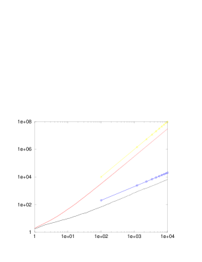
Figure 1: Log-log plot of the dispersions $\langle x^{2}(t)\rangle$ (lower curve) and $\langle y^{2}(t)\rangle$ corresponding to the flow (22), versus time. These curves were obtained by Monte-Carlo simulation. The asymptotic slopes are respectively 1 and 2, consistently with the fact that the ballistic velocity points in the $y$-direction. The values for the ballistic velocity generated in the simulation agree with the theoretical prediction (23).

For the sake of concreteness, let us consider in more detail the following simple periodic flow :

$${\mbox{\boldmath$v$}}=(\sin x\,;\,-\cos x).$$ (22)

The averages appearing in (21) can be calculated in terms of the Bessel functions $I_{0}$ and $I_{1}$ of imaginary argument. The relevant formulae, from [24], are listed for convenience in Appendix B. The final result is

$$\left(V_{b}\right)_{y}={I_{1}(1/\kappa)-I_{1}(-1/\kappa)\over I_{0}(1/\kappa)+I_{0}(-1/\kappa)}={I_{1}(1/\kappa)\over I_{0}(1/\kappa)}.$$ (23)

For large values of the molecular diffusivity $\kappa$, the Bessel functions can be expanded and

$$\left(V_{b}\right)_{y}={1\over 2\kappa}+O(1/\kappa^{2}),$$ (24)

which agrees with the general expression (A.7) derived in Appendix A. When $\kappa$ is small, we can use the asymptotic expansions (B.5) and (B.6) to obtain

$$\left(V_{b}\right)_{y}=1-{\kappa\over 2}+O(\kappa^{2}).$$ (25)

Both (24) and (25) can obviously be also obtained directly from (21). For small $\kappa$’s the field $m$ has a sharp maximum in $\pi$ around which it reduces to a Gaussian with variance $\kappa$. The result (25) is then obtained by using Laplace method. The expansion (25) is in agreement with the fact that $w(\pi)=1$ and molecular noise forbids the concentration of all particles in the minimum of the potential. A closer look at the streamlines of the flow reveals the very simple dynamics associated with the ballistic transport (22). The potential component concentrates the particles in the middle of the channel $(0,2\pi)$. Here, the solenoidal part $w$ transports the particles in the positive $\hat{y}$-direction. In the general case the mechanism is more complicated and cannot be treated analytically but this simple example highlights the essential role of both the solenoidal and the potential components for ballistic transport.

4.2 A cellular flow

Another velocity field such that the auxiliary equation (18) can also be tackled analytically, at least partially, is the following slightly perturbed cellular flow

$${\mbox{\boldmath$v$}}=(\cos y+\delta\cos x\,;\,\sin x)\equiv{\mbox{\boldmath$v$}}^{I}+\hat{\mbox{\boldmath$x$}}\delta\cos x.$$ (26)

The term proportional to the constant $\delta$ is a small compressible perturbation, while for $\delta=0$ the flow (26) reduces to the projection of the incompressible ABC flow [25] (with A=0, B=C=1) on the $x-y$ plane. We shall derive here the asymptotic expression of the effective velocity ${\mbox{\boldmath$V$}}_{b}$ valid for large Péclet numbers.

The incompressible BC flow ${\mbox{\boldmath$v$}}^{I}$ consists of square convective cells with separatrices parallel to the diagonals. The mechanism of effective diffusion at high Péclet numbers for this type of flow is well understood [8, 9]. Particles within the cells simply circulate along the streamlines and their density rapidly becomes almost uniform. On the contrary, particles close to the separatrices may cross the cell boundary because of molecular noise. The width of the layers where these transitions typically occur is proportional to $\sqrt{\kappa}$. For small $\kappa$, it is therefore possible to calculate the asymptotic behaviour of the effective diffusivity $\kappa^{E}$ by using boundary layer theory. The stream function of our BC flow ${\mbox{\boldmath$v$}}^{I}$ coincides with the one considered in Ref. [9] with the transformations

$$x^{\prime}={x+y\over\sqrt{2}}\,;\qquad y^{\prime}={x-y\over\sqrt{2}}-{\pi\over 2},$$ (27)

and $\tilde{u}=\sqrt{2}$, $d=\sqrt{2}\pi$, $\beta=1$ (see eqs. (2) and (3) in Ref. [9]). The corresponding expression of the effective diffusivity derived in Ref. [9] (eqs. (26) and (28)) is :

$$\kappa^{E}\simeq{2\over 0.749\sqrt{\pi}}\kappa^{1/2}.$$ (28)

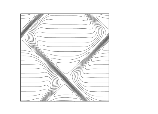
Figure 2: Contour lines of the function $m$ corresponding to the slightly perturbed flow (26), obtained by solving the auxiliary problem (18) numerically. The parameter values are $\delta=0.05$ and $\kappa=0.01$.

On the other hand, the effective diffusivity for the incompressible BC flow ${\mbox{\boldmath$v$}}^{I}$ can be expressed as (see, e.g., Ref. [10]) :

$$\kappa^{E}_{\alpha\beta}=\kappa\delta_{\alpha\beta}-{1\over 2}\left[\langle v^{I}_{\alpha}s_{\beta}\rangle+\langle v^{I}_{\beta}s_{\alpha}\rangle\right],$$ (29)

where $s$ has zero average value and satisfies

$$\partial_{t}\,{\mbox{\boldmath$s$}}+\left({\mbox{\boldmath$v$}}^{I}\cdot{\mbox{\boldmath$\partial$}}\right){\mbox{\boldmath$s$}}-\kappa\,\partial^{2}\,{\mbox{\boldmath$s$}}=-{\mbox{\boldmath$v$}}^{I}.$$ (30)

The effective diffusivity, which is in general a second-order tensor, reduces for the BC flow to a scalar thanks to the following symmetries :

$$x\mapsto y+{\pi\over 2}\,;\quad y\mapsto x-{\pi\over 2}\,;\quad v^{I}_{x}\mapsto v^{I}_{y}\,;\quad v^{I}_{y}\mapsto v^{I}_{x},$$ (31)

and

$$x\mapsto\pi-x\,;\quad y\mapsto y-\pi\,;\quad v^{I}_{x}\mapsto-v^{I}_{x}\,;\quad v^{I}_{y}\mapsto v^{I}_{y}.$$ (32)

An immediate consequence of (31) is that the diagonal components of the tensor in (29) are equal and the symmetry (32) implies that the non-diagonal components vanish. It follows that

$$\kappa^{E}=\kappa^{E}_{xx}=\kappa^{E}_{yy}=-\langle v^{I}_{y}s_{y}\rangle,$$ (33)

where $s_{y}$ is the zero-average solution of the equation

$$\partial_{t}\,s_{y}+\left({\mbox{\boldmath$v$}}^{I}\cdot{\mbox{\boldmath$\partial$}}\right)s_{y}-\kappa\,\partial^{2}\,s_{y}=-\sin x.$$ (34)

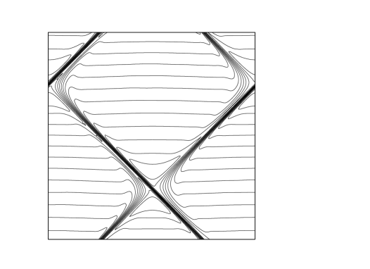
Figure 3: Same as in Figure 2, with parameters $\delta=0.05$ and $\kappa=0.001$.

The crucial remark is now that equation (34) coincides with the auxiliary equation (18) for the flow (26) at the dominant order in $\delta$. When the solution of (18) is sought as

$$m=m^{(0)}+\delta\,m^{(1)}+\delta^{2}\,m^{(2)}+\ldots,$$ (35)

it is easy to check that $m^{(0)}=1$ and $m^{(1)}=-s_{y}$. It follows from (17), (28) and (33) that the asymptotic behaviour of $\left(V_{b}\right)_{y}$ is

$$\left(V_{b}\right)_{y}\simeq{2\delta\over 0.749\sqrt{\pi}}\kappa^{1/2}+O(\delta^{2}).$$ (36)

Note that the behaviour in $\kappa$ of terms of higher order in $\delta$ is not under our control in this expansion.

The $x$-component of the ballistic velocity vanishes for arbitrary $\delta$ and $\kappa$. Independently of the value of $\delta$, the flow (26) has in fact the symmetry (32) :

$$x\mapsto\pi-x\,;\qquad y\mapsto y-\pi\,;\qquad v_{x}\mapsto-v_{x}\,;\qquad v_{y}\mapsto v_{y}.$$ (37)

By using (37) in (18), we immediately obtain

$$m(\pi-x\,;\,y-\pi)=m(x\,;\,y),$$ (38)

and

$$\left(V_{b}\right)_{x}=\langle v_{x}\,m\rangle=0.$$ (39)

The prediction (36) is compared in Table 1 to the values obtained by solving numerically the auxiliary equation (18) for the flow (26). The equation has been solved by using pseudo-spectral methods [26] and the parameter $\delta=0.05$. The contour plots of the field $m$ are shown in Figs. 2 and 3 for $\kappa=0.01$ and $\kappa=0.001$, respectively. The resolution is $256\times 256$, which ensures that the boundary layers are properly resolved.

	Spectral $64^{2}$	Asympt. Pred.
$\kappa$	$\left(V_{b}\right)_{y}$	$\left(V_{b}\right)_{y}$
$1.\times 10^{-1}$	$2.0\times 10^{-2}$	$2.4\times 10^{-2}$
$5.\times 10^{-2}$	$1.5\times 10^{-2}$	$1.7\times 10^{-2}$
$1.\times 10^{-2}$	$7.1\times 10^{-3}$	$7.5\times 10^{-3}$
$5.\times 10^{-3}$	$5.2\times 10^{-3}$	$5.3\times 10^{-3}$

Table 1: The $y$-component of the ballistic velocity $\left(V_{b}\right)_{y}$ for the flow (26) with $\delta=0.05$.

It is evident that the quality of the prediction (36) improves when $\kappa$ is decreased. This is in agreement with the asymptotic nature of the boundary-layer technique which has been used in the calculations.

4.3 Random flows with short correlation times

It is known that the effective diffusivity for incompressible flow with short-correlation times can be calculated exactly (see, e.g., Ref. [10]). The aim of this Section is to show that short correlation times also allow to calculate the effective ballistic velocity for compressible flow.

Specifically, the velocity field is supposed to be a homogeneous, Gaussian random process having zero average value and correlation function

$$\langle v_{\alpha}({\mbox{\boldmath$x$}},t)\,v_{\beta}({\mbox{\boldmath$0$}},t^{\prime})\rangle=F_{\alpha\beta}({\mbox{\boldmath$x$}})\,\delta(t-t^{\prime}).$$ (40)

In order to calculate the average (17) we can now use the formula of Gaussian integration by parts (see, e.g., Refs. [27, 28]). The average is then expressed as

$${\mbox{\boldmath$V$}}_{b}=\langle m{\mbox{\boldmath$v$}}\rangle=\int\,d{\mbox{\boldmath$x$}}^{\prime}\,dt^{\prime}\langle{\mbox{\boldmath$v$}}({\mbox{\boldmath$x$}},t){\mbox{\boldmath$v$}}({\mbox{\boldmath$x$}}^{\prime},t^{\prime})\rangle\langle{\delta m({\mbox{\boldmath$x$}},t)\over\delta{\mbox{\boldmath$v$}}({\mbox{\boldmath$x$}}^{\prime},t^{\prime})}\rangle.$$ (41)

From the auxiliary eq. (18) and the $\delta$-correlation in time it immediately follows

$${\mbox{\boldmath$V$}}_{b}=-\int_{0}^{\infty}\langle{\mbox{\boldmath$v$}}({\mbox{\boldmath$x$}},t)\left({\mbox{\boldmath$\partial$}}\cdot{\mbox{\boldmath$v$}}\right)({\mbox{\boldmath$x$}},0)\rangle\,dt,$$ (42)

where the stochastic differential equation (18) is interpreted à la Stratonovich since we are interested in the physical limit of short correlation times. Eq. (42) had already been derived in Ref. [22] using path-integral methods. Note that the average appearing in (42) vanishes for incompressible flow. It also vanishes for parity-invariant and isotropic flow, in agreement with the results of the next Section.

An alternative derivation of (42) is to neglect the diffusive term in the auxiliary equation (18) and integrate on the characteristics :

$$m({\mbox{\boldmath$x$}},t)={\exp\left(-\int_{-\infty}^{t}({\mbox{\boldmath$\partial$}}\cdot{\mbox{\boldmath$v$}})({\mbox{\boldmath$x$}}({\mbox{\boldmath$a$}},s)\,;\,s)\,ds\right)\over\langle\exp\left(-\int_{-\infty}^{t}({\mbox{\boldmath$\partial$}}\cdot{\mbox{\boldmath$v$}})({\mbox{\boldmath$x$}}({\mbox{\boldmath$a$}},s)\,;\,s)\,ds\right)\rangle}.$$ (43)

The characteristics are the Lagrangian trajectories defined by the equation

$${d{\mbox{\boldmath$x$}}({\mbox{\boldmath$a$}},t)\over dt}={\mbox{\boldmath$v$}}({\mbox{\boldmath$x$}}({\mbox{\boldmath$a$}},t)\,;\,t),$$ (44)

where $a$ is the initial position of the particle. In (43) the integration has to made on the trajectory such that ${\mbox{\boldmath$x$}}({\mbox{\boldmath$a$}},t)={\mbox{\boldmath$x$}}$. Inserting (43) into (17) we obtain an expression of the ballistic velocity as time integral of Lagrangian correlations. This is the equivalent of Taylor’s formula for effective diffusivities. The presence of the exponential makes it however very difficult to use. When the flow has a short correlation time one can however simplify (43) by exploiting the fact that Lagrangian and Eulerian statistics tend to coincide. Using again Gaussian integration by parts (42) immediately follows.

5 General conditions for the absence of ballistic    transport

The aim of this Section is to identify some general classes of flows where ballistic transport is absent and pure diffusion takes place.

A first class where ${\mbox{\boldmath$V$}}_{b}=0$ is the one of incompressible flow. This has already been shown by (14) in Section 3.

Let us then consider parity-invariant flow, i.e. velocity fields having at least one center of symmetry according to the definition (8) in Section 2. It follows from (8) that the solution $m$ of (18) having unit average value satisfies

$$m(-{\mbox{\boldmath$x$}},t)=m({\mbox{\boldmath$x$}},t).$$ (45)

In the random case, the statistics is invariant under the operations

$${\mbox{\boldmath$x$}}\mapsto-{\mbox{\boldmath$x$}}\,;\qquad{\mbox{\boldmath$v$}}\mapsto-{\mbox{\boldmath$v$}}\,;\qquad m\mapsto m.$$ (46)

An immediate consequence of (8) and (45) (or (46) for the random case) is the vanishing of the ballistic velocity ${\mbox{\boldmath$V$}}_{b}=0$.

To give a direct confirmation of these considerations we present in Fig. 4 the dispersions for the flow

$${\mbox{\boldmath$v$}}=(\sin x\,;\,\sin x+\sin 3x).$$ (47)

This flow depends on a single coordinate as discussed in Section 4.1. Unlike (22), the flow (47) has however the center of symmetry $x=\pi$. It follows then that ballistic transport is forbidden. The difference is best appreciated by comparing Figs. 1 and 4. In the first case $\langle y^{2}(t)\rangle\propto t^{2}$ while in Fig. 4 $\langle y^{2}(t)\rangle\propto t$, corresponding to diffusive transport.

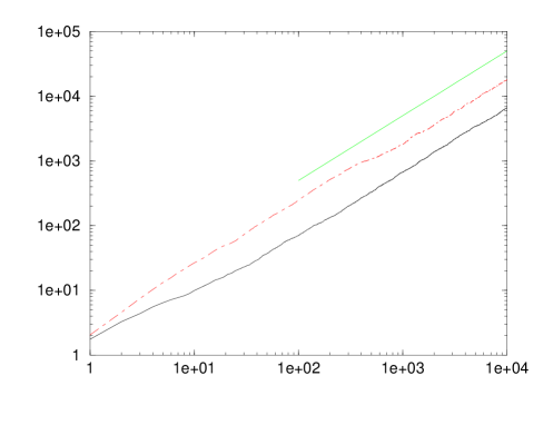
Figure 4: The dispersions $\langle x^{2}(t)\rangle$ (lower curve) and $\langle y^{2}(t)\rangle$ for the flow (47). The straight line is proportional to $t$.

We consider now homogeneous and isotropic random flow. These flows are defined, According to the definition in [29], these flows are such that their statistical properties are unaffected by translations and/or rotations accompanied by a simultaneous rotation of the laboratory frame. Note that, unlike the definition in Ref. [29], we distinguish here between isotropy and statistical parity-invariance, e.g. a 3D helical flow can be isotropic even if it is not parity-invariant. Since no preferential direction but $v$ appears in (18), the statistical properties of the couple $(m,{\mbox{\boldmath$v$}})$ are invariant under rotations. Homogeneity and the absence of a preferential direction imply then that the single-point correlation

$${\mbox{\boldmath$V$}}_{b}=\langle{\mbox{\boldmath$v$}}({\mbox{\boldmath$x$}},t)\,m({\mbox{\boldmath$x$}},t)\rangle=0.$$ (48)

In practice, information on isotropy or parity-invariance of the flow may not be available. To check whether ballistic transport is present one could then use the expansion in powers of ${1\over\kappa}$ derived in Appendix B. To leading order, this expansion shows that

$${\mbox{\boldmath$V$}}_{b}\ =\ -{1\over\kappa}\cdot\langle{\mbox{\boldmath$v$}}{\cal H}^{-1}\left({\mbox{\boldmath$\partial$}}\cdot{\mbox{\boldmath$v$}}\right)\rangle+\ O\left({1\over\kappa^{2}}\right)\ ,$$ (49)

where ${\cal H}^{-1}\ =\ \left(\partial_{\tau}-\partial^{2}\right)^{-1}$ is the Green’s function of the heat diffusion operator. For time-independent flows, the latter expression reduces to

$${\mbox{\boldmath$V$}}_{b}\ =\ -{1\over\kappa}\cdot\langle{\mbox{\boldmath$v$}}^{I}\,\phi\rangle+\ O\left({1\over\kappa^{2}}\right)\ ,$$ (50)

where ${\mbox{\boldmath$v$}}^{I}$ represents the incompressible component of the velocity field and $\phi$ the potential of the irrotational component. The averages in the asymptotic expressions (49) or (50) are easy to measure and can be used to estimate whether the ballistic drift is present or not.

Finally, we investigate time-independent potential velocity fields, i.e. satisfying

$${\mbox{\boldmath$v$}}({\mbox{\boldmath$x$}})=-{\mbox{\boldmath$\partial$}}\phi({\mbox{\boldmath$x$}}),$$ (51)

where $\phi$ is the potential. The stationary solution of (18) for this class of flows is the Boltzmann distribution (see, e.g., Ref. [20]) :

$$m={\exp\left(-{\phi\over\kappa}\right)\over\langle\exp\left(-{\phi\over\kappa}\right)\rangle}.$$ (52)

It follows from periodicity (or homogeneity) that

$${\mbox{\boldmath$V$}}_{b}\propto\,\langle{\mbox{\boldmath$v$}}\exp\left(-{\phi\over\kappa}\right)\rangle\,=\,\kappa\langle{\mbox{\boldmath$\partial$}}\left(\exp\left(-{\phi\over\kappa}\right)\right)\rangle\,=\,0.$$ (53)

Ballistic effect is therefore impossible for time-independent potential flow. Note that the condition of time-independence is essential for this result. Indeed, if $\phi$ depends on time the solution of (18) is not the Boltzmann distribution. Furthermore, let us consider the one-dimensional flow

$$v(x,t)=\cos(x-\kappa\,\omega\,t)+a\cos(x+\kappa\,\omega\,t).$$ (54)

Using (A.5) in Appendix A, it is easy to check that the first coefficient of the perturbative expansion in $1/\kappa$ of the ballistic velocity is

$$V_{b}=\left({\omega\over 1+\omega^{2}}{1-a^{2}\over 2}\right){1\over\kappa}+O\left({1\over\kappa^{2}}\right).$$ (55)

The fact that (55) does not vanish illustrates the fact that ballistic transport is possible for time-dependent potential flow. One can also easily check that the expression (42), valid for compressible $\delta$-correlated flow, does not generally vanishes for potential flow.

6 Effective diffusivities for compressible flow

In the previous Section we have considered advective effects in large-scale transport by compressible flow. It is physically clear that diffusive effects will also be present. In order to systematically treat them, multi-scale techniques can again be used. To capture both advective and diffusive effects, two independent slow times $T_{1}=\epsilon t$ and $T_{2}=\epsilon^{2}t$ are needed. The solvability condition at order $\epsilon$ gives the advective effects, as shown in Section 3, while at order $\epsilon^{2}$ we also include diffusive effects (see Ref. [2]). For the flows where the ballistic velocity ${\mbox{\boldmath$V$}}_{b}$ vanishes, no advective time is needed. The formalism is then the same as in Section 3, with the only difference that the slow time is now defined as $T=\epsilon^{2}t$. Since there are just technical differences between the two cases ${\mbox{\boldmath$V$}}_{b}\neq 0$ and ${\mbox{\boldmath$V$}}_{b}=0$, we shall treat in detail the latter and give only the final results for the former.

As in Section 3 we denote the fast variables by $x$, $t$ and the slow space variable is defined as ${\mbox{\boldmath$X$}}=\epsilon{\mbox{\boldmath$x$}}$. The analogous of equation (9) for the derivatives is now :

$$\partial_{i}\mapsto\partial_{i}+\epsilon\nabla_{i}\,\,\,,\qquad\partial_{t}\mapsto\partial_{t}+\epsilon^{2}\partial_{T}\,\,\,,$$ (56)

The solution $\Theta$ of the Fokker-Planck equation (4) is again sought in the form of a series in $\epsilon$. When (56) and (10) are inserted into (4), a hierarchy of equations of the form (11) is recovered. For the analysis of turbulent diffusion the following three equations are needed :

$${\cal A}\Theta^{(0)} = 0\,,$$ (57)

$${\cal A}\Theta^{(1)} = -{\mbox{\boldmath$v$}}\cdot\nabla\Theta^{(0)}+2\kappa{\mbox{\boldmath$\partial$}}\cdot\nabla\Theta^{(0)}\,,$$ (58)

$${\cal A}\Theta^{(2)} = -\partial_{T}\Theta^{(0)}-{\mbox{\boldmath$v$}}\cdot\nabla\Theta^{(1)}+2\kappa{\mbox{\boldmath$\partial$}}\cdot\nabla\Theta^{(1)}+\kappa\nabla^{2}\Theta^{(0)}.$$ (59)

The operator ${\cal A}$ is defined by (11). Using the linearity of (57), we can express the solution as in (15), where the field $m$ satisfies (18). We can then insert (15) into (58). Using again the linearity of the operator ${\cal A}$, we obtain:

$$\Theta^{(1)}={\mbox{\boldmath$\chi$}}\cdot\nabla\langle\Theta^{(0)}\rangle+\,m\langle\Theta^{(1)}\rangle.$$ (60)

where the vector field $\chi$ satisfies

$$\partial_{t}{\mbox{\boldmath$\chi$}}+\underline{{\mbox{\boldmath$\partial$}}}\cdot\left(\underline{{\mbox{\boldmath$v$}}}{\mbox{\boldmath$\chi$}}\right)-\kappa\,\partial^{2}{\mbox{\boldmath$\chi$}}=-{\mbox{\boldmath$v$}}\,m+2\kappa\,{\mbox{\boldmath$\partial$}}\,m.$$ (61)

The underline in the l.h.s. of (61) is meant to make it clear that in the scalar product the components of $\partial$ have to be contracted only with those of $v$, and not of $\chi$. As expected, the solvability condition for (61) requires ${\mbox{\boldmath$V$}}_{b}=0$ (which we have supposed to be true). In the cases when ${\mbox{\boldmath$V$}}_{b}$ does not vanish, the calculations with the two-times formalism give the following modified equation

$$\partial_{t}{\mbox{\boldmath$\chi$}}+\underline{{\mbox{\boldmath$\partial$}}}\cdot\left(\underline{{\mbox{\boldmath$v$}}}{\mbox{\boldmath$\chi$}}\right)-\kappa\,\partial^{2}{\mbox{\boldmath$\chi$}}=-m\,\left({\mbox{\boldmath$v$}}-{\mbox{\boldmath$V$}}_{b}\right)+2\kappa\,{\mbox{\boldmath$\partial$}}\,m,$$ (62)

where ${\mbox{\boldmath$V$}}_{b}$ is given by (17). Eq. (61) is clearly a particular case of (62).

The equation for the large scales dynamics emerges as the solvability condition for (59)

$$\partial_{T}\langle\Theta^{(0)}\rangle=\kappa^{E}_{\alpha\beta}\nabla_{\alpha}\nabla_{\beta}\langle\Theta^{(0)}\rangle,$$ (63)

where the effective diffusivity tensor is

$$\kappa^{E}_{\alpha\beta}=\kappa\delta_{\alpha\beta}-{1\over 2}\left[\langle v_{\alpha}\chi_{\beta}\rangle+\langle v_{\beta}\chi_{\alpha}\rangle\right].$$ (64)

When ${\mbox{\boldmath$V$}}_{b}\neq 0$, the effective equation for the mean value of the field becomes

$$\partial_{T}\langle\Theta^{(0)}\rangle+{\mbox{\boldmath$V$}}_{b}\cdot\nabla\langle\Theta^{(0)}\rangle=\kappa^{E}_{\alpha\beta}\nabla_{\alpha}\nabla_{\beta}\langle\Theta^{(0)}\rangle,$$ (65)

where the effective diffusivity has the expression (64) and the $\chi$ field is the solution of (62).

The diffusivity tensor $\kappa^{E}_{\alpha\beta}$ might of course be anisotropic, reflecting the fact that the flow could be non-invariant under arbitrary rotations. The term in the square parentheses in (64) does not have a definite sign for generic compressible flow. The quantity $\kappa^{E}-\kappa$ is in fact known to be positive for incompressible flow and in the next Section we show that it is always negative for static potential flow (see also the following example).

There are some special instances where the effective diffusivity can be calculated analytically, e.g. the flows of the class (19). We shall not dwell on the details here since the solution of (18) is the Boltzmann distribution (20) and the solution of (61) is essentially the same as the one which will be discussed in Section 7.2. The final result is that $\kappa^{E}_{xx}$ is given by (80), the non-diagonal components vanish and

$$\kappa^{E}_{yy}=\kappa+{\langle e^{\phi/\kappa}\rangle\over\kappa}\langle\left(\psi-{\langle\psi e^{\phi/\kappa}\rangle\over\langle e^{\phi/\kappa}\rangle}\right)^{2}\left({e^{\phi/\kappa}\over<e^{\phi/\kappa}>}\right)\rangle,$$ (66)

which is clearly larger than $\kappa$. The function $\psi$ is defined by

$$\psi(x)=\int_{0}^{x}w(z)\exp\left(-{\phi(z)\over\kappa}\right)\,dz,$$ (67)

and it is still a periodic function since the ballistic velocity is supposed to vanish.

For generic compressible flow, the solutions of the auxiliary equations (18) and (61) are not generally known and one should then resort to numerical methods, as in the incompressible case [10, 11].

7 Static potential flow

One of the results derived in Section 5 is that no ballistic transport is possible for static potential flow. In the presence of scale separation, transport by these flows is therefore always diffusive. This is rather intuitive from a physical point of view. Particles are indeed concentrated into the minima of the potential where the velocity however vanishes. For the flow in Section 4.1 one immediately realizes, for example, that without the streaming in the $\hat{y}$-direction due to the solenoidal part no ballistic advection would be possible. As a matter of fact, we expect that even diffusion should be very sensitive to the presence of potential wells. Let us indeed consider a stagnation point ${\mbox{\boldmath$x$}}_{0}$ (${\mbox{\boldmath$v$}}({\mbox{\boldmath$x$}}_{0})=0$) and the quantity

$${\cal T}={\mbox{\boldmath$v$}}({\mbox{\boldmath$x$}})\cdot({\mbox{\boldmath$x$}}-{\mbox{\boldmath$x$}}_{0}).$$ (68)

When ${\cal T}$ is expanded in a Taylor series, the first non-zero term is generically quadratic :

$${\cal T}\simeq S_{ij}({\mbox{\boldmath$x$}}-{\mbox{\boldmath$x$}}_{0})_{i}\,({\mbox{\boldmath$x$}}-{\mbox{\boldmath$x$}}_{0})_{j}={1\over 2}\left(\partial_{i}v_{j}+\partial_{j}v_{i}\right)({\mbox{\boldmath$x$}}-{\mbox{\boldmath$x$}}_{0})_{i}\,({\mbox{\boldmath$x$}}-{\mbox{\boldmath$x$}}_{0})_{j}.$$ (69)

In order to have strong trapping the velocity field should be such that the particles are driven back to ${\mbox{\boldmath$x$}}_{0}$, i.e. ${\cal T}<0$ everywhere in a neighbourhood of ${\mbox{\boldmath$x$}}_{0}$. This is by definition what happens in the minima of the potential $\phi$ for the flows (51). On the contrary, this strong form of trapping is impossible for incompressible flow. The tensor $S$ is in fact traceless and not all its eigenvalues can be negative. The conclusion of these simple heuristic arguments is that a depletion of transport is expected for static potential flow. This expectation is confirmed by the systematic results of the next Section showing that the effective diffusivity is indeed smaller than the molecular diffusivity.

7.1 Depletion of transport

For static potential velocity fields of the class (51) the calculation of the effective diffusivity can be reduced to the solution of one auxiliary equation only. We can then show that diffusive transport is always depleted.

The solution of the first auxiliary equation (57) is the Boltzmann distribution :

$$\Theta^{(0)}=\langle\Theta^{(0)}\rangle({\mbox{\boldmath$X$}},T)\,\,{\exp\left(-{\phi\over\kappa}\right)\over\langle\exp\left(-{\phi\over\kappa}\right)\rangle}.$$ (70)

Inserting (70) into (61), we obtain :

$$\partial_{t}{\mbox{\boldmath$\Xi$}}+\underline{{\mbox{\boldmath$\partial$}}}\cdot\left(\underline{{\mbox{\boldmath$v$}}}\,{\mbox{\boldmath$\Xi$}}\right)-\kappa\,\partial^{2}{\mbox{\boldmath$\Xi$}}=\kappa\,{\mbox{\boldmath$\partial$}}\left(\exp\left({-{\phi\over\kappa}}\right)\right),$$ (71)

where ${\mbox{\boldmath$\Xi$}}={\mbox{\boldmath$\chi$}}\langle\exp\left(-{\phi\over\kappa}\right)\rangle$ and has zero average value. It is then convenient to define

$${\mbox{\boldmath$\Upsilon$}}=\exp\left({\phi\over\kappa}\right){\mbox{\boldmath$\Xi$}}.$$ (72)

The equation for $\Upsilon$ is easily derived from (71)

$$\partial_{t}{\mbox{\boldmath$\Upsilon$}}-\left({\mbox{\boldmath$v$}}\cdot{\mbox{\boldmath$\partial$}}\right)\,{\mbox{\boldmath$\Upsilon$}}-\kappa\,\partial^{2}{\mbox{\boldmath$\Upsilon$}}={\mbox{\boldmath$v$}}.$$ (73)

We can now recast the averages appearing in the expression of the effective diffusivity (64) in a more convenient form. Let us indeed multiply the components $\alpha$ and $\beta$ of (73) by $\Xi_{\beta}$ and $\Xi_{\alpha}$, respectively. By summing, taking the average and using the definitions of $\Xi$ and $\Upsilon$, we obtain after some algebra :

$$-{1\over 2}\left[\langle v_{\alpha}\,{\mbox{\boldmath$\chi$}}_{\beta}\rangle+\langle v_{\beta}\,{\mbox{\boldmath$\chi$}}_{\alpha}\rangle\right]=-\kappa\langle\exp\left(-{\phi\over\kappa}\right)({\mbox{\boldmath$\partial$}}\Upsilon_{\alpha})\cdot({\mbox{\boldmath$\partial$}}\Upsilon_{\beta})\rangle\,/\langle\exp\left(-{\phi\over\kappa}\right)\rangle.$$ (74)

In order to derive this equality we have used the periodicity (or homogeneity) of $v$. It is evident from (74) that the correction to the molecular value which appears on the r.h.s. of (64) is negative definite. This proves that transport is always depleted.

Let us then show that, despite of the fact that the correction due to the flow $v$ is negative, the whole effective diffusivity $\kappa^{E}_{\alpha\beta}$ is still positive, i.e. the absolute value of the correction is always smaller than $\kappa$. Inserting the expression of $\chi$ in terms of $\Upsilon$ into (64) and integrating by parts we have

$$|\delta\kappa|\equiv\left(\kappa\delta_{\alpha\beta}-\kappa^{E}_{\alpha\beta}\right)n_{\alpha}n_{\beta}=\kappa{\langle\exp\left(-{\phi\over\kappa}\right)\partial_{\parallel}({\mbox{\boldmath$\Upsilon$}}\cdot\hat{n})\rangle\over\langle\exp\left(-{\phi\over\kappa}\right)\rangle},$$ (75)

where $\hat{n}$ is a generic direction and $\partial_{\parallel}=(\hat{n}\cdot{\mbox{\boldmath$\partial$}})$. Using the Schwartz inequality leads to

$$|\delta\kappa|\leq\kappa{\langle\exp\left(-{\phi\over\kappa}\right)(\partial_{\parallel}({\mbox{\boldmath$\Upsilon$}}\cdot\hat{n}))^{2}\rangle^{1/2}\over\langle\exp\left(-{\phi\over\kappa}\right)\rangle^{1/2}}\leq\kappa{\langle\exp\left(-{\phi\over\kappa}\right)({\mbox{\boldmath$\partial$}}({\mbox{\boldmath$\Upsilon$}}\cdot\hat{n}))^{2}\rangle^{1/2}\over\langle\exp\left(-{\phi\over\kappa}\right)\rangle^{1/2}}=\sqrt{\kappa|\delta\kappa|}.$$ (76)

Equation (74) has been used to derive the last equality. The consequence of (76) is that the effective diffusivity tensor $\kappa^{E}_{\alpha\beta}$ is indeed positive definite, in agreement with the known fact that the original Fokker-Planck equation is stable [20].

We have then shown that a static potential flow always leads to depletion of transport. This should be contrasted to the case of incompressible flow, where transport properties are always enhanced. Remark that for time-dependent potential flow the result just proved does not generally hold. The time-dependence can in fact destroy the trapping effects due to potential wells and lead to an enhancement of transport. One can easily provide an explicit example by taking again the flow (54) with $a=1$ (the flow is then parity-invariant and no ballistic effect is present). The analytic expression of the effective diffusivity is not known. For our aims it is however enough to perform an expansion for large $\kappa$ quite similar to the one presented in Appendix A. The first term of the expansion of $\kappa^{E}$ is obtained by some simple algebra :

$$\kappa^{E}=\kappa+{1\over\kappa}{\omega^{2}-3\over(\omega^{2}+1)^{2}}+O(1/\kappa^{2}).$$ (77)

The fact that $\kappa^{E}$ can be either larger or smaller than $\kappa$ indicates that no general rule can be expected. Enhancement or depletion of transport properties are both possible, depending on the detailed structure of the flow.

7.2 The one-dimensional case

The calculation of the effective diffusivity has been reduced to the solution of the auxiliary equation (71). While in the multi-dimensional case no general solution is known, the equation can be solved analytically in 1D. The reason for this simplification is that in one dimension the order of the equation can be lowered, thus reducing it to a first-order differential equation. We shall consider in detail the case of periodic, deterministic flow. The random case is handled similarly.

It follows from equation (73) that

$${d\over dx}(\Upsilon+x)=c\exp\left({\phi\over\kappa}\right),$$ (78)

where $c$ is a constant and $x$ is the spatial coordinate. One more integration leads to

$$\Upsilon=c\,\int_{0}^{x}\exp\left({\phi\over\kappa}\right)\,dy\,\,+\,\,c^{\prime}\,-\,x.$$ (79)

The constants $c$ and $c^{\prime}$ are fixed by imposing the conditions that the function $\chi$ appearing in (72) is periodic and has zero average. For the calculation of $\kappa^{E}$ only the value of $c$ turns out to be actually needed. By imposing the periodicity of (79), we finally obtain the expression of the effective diffusivity :

$$\kappa^{E}={\kappa\over\langle\exp({\phi\over\kappa})\rangle\langle\exp(-{\phi\over\kappa})\rangle}.$$ (80)

It follows from (80) that for small values of the molecular diffusivity the ratio $\kappa^{E}/\kappa$ is exponentially small and has the structure of an Arrhenius factor. The term in (80) is indeed proportional to the probability for a particle to jump out of a well of depth equal to the difference between the absolute maximum and minimum of the potential (see e.g. Section 5.10 in Ref. [20]). The mechanism of transport is thus essentially a random walk between the minima of the potential. Particles are trapped for very long times in the bottom of potential wells. Because of large fluctuations in the noise, they can occasionally jump out of a minimum falling into the adjacent one. The same mechanism evidently works also in the multidimensional case and is responsible for the depletion of transport found in Section 7.1.

For Gaussian random flow the averages in (80) can be easily calculated :

$${\kappa^{E}\over\kappa}=\exp\left(-{\langle\phi^{2}\rangle\over\kappa^{2}}\right).$$ (81)

Note that for transport to be diffusive at sufficiently large scales, the condition

$$\langle\phi^{2}\rangle\quad<\infty,$$ (82)

must be satisfied. When (82) is not satisfied, the hypothesis of scale separation breaks down. The small-scale typical time for relaxation to local equilibrium is indeed of the order of the typical Arrhenius time needed to jump out of the wells. When (82) is violated, this time is divergent because wells of arbitrary depth are present. There is therefore no time which is much larger than the typical times of the small-scale dynamics. Standard diffusion is never observed and transport is sub-diffusive. An explicit example is provided by the case when $\phi$ is a Brownian motion. Ya. Sinai found in Refs. [31, 32] that in this case the dispersion does not vary linearly with time but

$$\langle(x(a,t)-x(a,0))^{2}\rangle\sim(\log t)^{4}.$$ (83)

Condition (82) is not satisfied also when $\phi$ is a fractional Brownian motion. This problem together with other examples of anomalous subdiffusive behavior and applications to statistical mechanics systems are discussed in detail in Ref. [33].

8 Conclusions

Turbulent transport by compressible flow has been investigated. For generic compressible flow having non-vanishing solenoidal and potential components, ballistic transport typically takes place. For isotropic and/or parity-invariant flow the ballistic velocity vanishes and transport is diffusive. The properties of the effective diffusivities are strongly dependent on the compressibility of the flow. For incompressible flow it is known that diffusion is always enhanced in the presence of small-scale velocity fields. On the contrary, we show that for static potential flow the effective diffusivities are reduced with respect to their molecular value. Trapping effects due to potential wells are responsible for this depletion. For time-dependent potential flow and generic compressible flow, depletion or enhancement of transport are both possible. No general rule can be drawn and the type of transport depends on the precise structure of the flow. An essential role is in particular played by the geometry of channels and stagnation points of the velocity field.

Appendices

Appendix A Expansion of the ballistic velocity for large      molecular diffusivities

In the limit of large molecular diffusivities $\kappa$, the ballistic velocity can be expressed as a perturbative series

$${\mbox{\boldmath$V$}}_{b}=\sum_{n=1}^{\infty}{{\mbox{\boldmath$c$}}^{(n)}\over\kappa^{n}}.$$ (A.1)

The vector coefficients ${\mbox{\boldmath$c$}}^{(n)}$ are defined by

$${\mbox{\boldmath$c$}}^{(n)}=\langle{\mbox{\boldmath$v$}}\,m^{(n)}\rangle,$$ (A.2)

where the functions $m^{(n)}$ are obtained recursively as

$$m^{(n+1)}=-{\cal H}^{-1}\,{\mbox{\boldmath$\partial$}}\cdot\left({\mbox{\boldmath$v$}}\,m^{(n)}\right)\qquad n\geq 1,$$ (A.3)

and $m^{(0)}=1$. The operator ${\cal H}$ is the heat operator

$${\cal H}=\partial_{\tau}-\partial^{2},$$ (A.4)

and $\tau=\kappa t$. The recursion relation (A.3) is simply obtained by applying the inverse of the heat operator to (18) and expanding in powers of $1/\kappa$. Note that for periodic, deterministic flow no problem in the inversion of ${\cal H}$ is encountered. The kernel of the operator is in fact made up of constants which however cannot show up in the r.h.s. of (A.3) because of the divergence operator. In the random case the convergence of the integrals involved in the coefficients ${\mbox{\boldmath$c$}}^{(n)}$ depends on the specific behaviour of the correlation functions of $v$. The first coefficient in (A.1) can be easily calculated

$${\mbox{\boldmath$c$}}^{(1)}=-\langle{\mbox{\boldmath$v$}}{\cal H}^{-1}\left({\mbox{\boldmath$\partial$}}\cdot{\mbox{\boldmath$v$}}\right)\rangle.$$ (A.5)

The velocity field $v$ can be generally decomposed as the sum of a potential and a solenoidal part

$${\mbox{\boldmath$v$}}=-{\mbox{\boldmath$\partial$}}\phi+{\mbox{\boldmath$v$}}^{I},$$ (A.6)

where ${\mbox{\boldmath$v$}}^{I}$ is divergence-free. For time-independent flow, (A.5) can be then reduced to the interesting form

$${\mbox{\boldmath$c$}}^{(1)}=-\langle\phi\,{\mbox{\boldmath$v$}}^{I}\rangle,$$ (A.7)

which illustrates the importance of correlations between the potential and the solenoidal components of the velocity field for ballistic transport.

Appendix B Some useful formulae

In this Appendix we list the formulae which are needed for the calculation in Section 4 of the ballistic velocity for the flow (22). The formulae are taken from [24].

$$\int_{0}^{\pi}\exp(-\beta\cos x)\,\cos x\,dx=i\pi\,J_{1}(i\beta)\,;$$ (B.1)

$$\int_{0}^{\pi}\exp(-\beta\cos x)\,dx=\pi\,J_{0}(i\beta)\,;$$ (B.2)

$$J_{n}(iz)=i^{n}I_{n}(z)\,;$$ (B.3)

$$I_{n}(z)=\sum_{k=0}^{\infty}{\left(z/2\right)^{2k+n}\over k!\,(k+n)!}\,;$$ (B.4)

$$I_{n}(x)\sim{e^{x}\over\sqrt{2\pi x}}\sum_{k=0}^{\infty}{(-1)^{k}\over(2x)^{k}}{\Gamma(n+k+1/2)\over k!\,\Gamma(n-k+1/2)}\,;$$ (B.5)

$$I_{n}(-x)\sim{e^{x}\over\sqrt{2\pi x}}e^{in\pi}\sum_{k=0}^{\infty}{(-1)^{k}\over(2x)^{k}}{\Gamma(n+k+1/2)\over k!\,\Gamma(n-k+1/2)}\,.$$ (B.6)

The functions $J_{n}$ and $I_{n}$ denote the Bessel functions of real and imaginary arguments, respectively. In both (B.4) and (B.5) the variable $x$ is supposed to be real, large and positive. The two couples of formulae (B.1), (B.2) and (B.5), (B.6) correspond to 3.915 and 8.451 in [24]. The (B.3) and (B.4) are 8.406 and 8.445.

References

- [1] U. Frisch, B. Hasslacher & Y. Pomeau, Phys. Rev. Lett., 56, 1505 , (1986).
- [2] U. Frisch, D. d’Humières, B. Hasslacher, P. Lallemand, Y, Pomeau & J.P. Rivet, Complex Systems, 1, 649 , (1987); also reproduced in Lattice Gas Methods For Partial Differential Equations. Ed. G.D, Doolen, Addison-Wesley, pp. 77.
- [3] H.K. Moffatt, Rep. Prog. Phys., 46, 621, (1983).
- [4] C.M. Bender & S.A. Orszag, Advanced Mathematical Methods for Scientists and Engineers (McGraw-Hill, 1978).
- [5] A. Bensoussan, J.-L. Lions & G. Papanicolaou, Asymptotic Analysis for Periodic Structures, (North-Holland, Amsterdam, 1978).
- [6] D. Mc Laughlin, G.C. Papanicolaou & O. Pironneau, SIAM Journal of Appl. Math., 45, 780, (1985).
- [7] Ya.B. Zeldovich, Sov. Phys. Dokl., 27, 10, (1982).
- [8] B.I. Shraiman, Phys. Rev. A, 36, 261, (1987).
- [9] M.N. Rosenbluth, H.L. Berk, I. Doxas & W. Horton, Phys. Fluids, 30, 2636, (1987).
- [10] L. Biferale, A. Crisanti, M. Vergassola & A. Vulpiani, Phys. Fluids, 7, 2725, (1995).
- [11] A. Majda & R. McLaughlin, Stud. Appl. Math,, 89, 245, (1993).
- [12] A. Fannjang & G.C. Papanicolaou, SIAM J. Appl. Math., 54, 333, (1994).
- [13] M. Avellaneda & A. Majda, Commun. Math. Phys., 138, 339, (1991).
- [14] M. Avellaneda & M. Vergassola, Phys. Rev. E, 52, 3249, (1995).
- [15] U. Frisch, Z.S. She, and P.L. Sulem, Physica, D28, 382, (1987).
- [16] G.I. Sivashinsky, Physica, D17, 243, (1985).
- [17] S. Gama, M. Vergassola & U. Frisch, J. Fluid Mech., 260, 95, (1994).
- [18] M. Vergassola, Europhys. Lett, 24, 41, (1993).
- [19] R. Benzi, A. Manfroi & M. Vergassola, Europhys. Lett, 36, 367, (1996).
- [20] H. Risken, The Fokker-Planck Equation, (Springer-Verlag, 1984).
- [21] H.K. Moffatt, Magnetic Field Generation in Electrically Conducting Fluids, (Cambridge Univ. Press, 1978).
- [22] T. Elperin, N. Kleeorin & I. Rogachevskii, Phys. Rev E, 52, 2617, (1995).
- [23] N.W. Aschcroft & N.D. Mermin, Solid State Physics, (Holt-Saunders, 1976).
- [24] I.S. Gradshteyn & I.M. Ryzhik, Tables of Integrals, Series and Products, (Academic Press, 1965).
- [25] T. Dombre, U. Frisch, J.M. Greene, M. Hénon, A. Mehr & A.M. Soward, J. Fluid Mech., 167, 353 (1986).
- [26] D. Gottlieb & S.A. Orszag. Numerical Analysis of Spectral Methods, SIAM, (1977).
- [27] U. Frisch, Turbulence, Cambridge Univ. Press, Cambridge, (1995).
- [28] J. Zinn-Justin, Quantum Field Theory and Critical Phenomena, Clarendon Press, Oxford, Second Edition (1993).
- [29] A.S. Monin & A.M. Yaglom, Statistical Fluid Mechanics, edited by J. Lumley, (MIT Press, Cambridge, Mass.) 1975.
- [30] R.H. Kraichnan, Phys. Fluids, 13, 22, (1970).
- [31] Ya.G. Sinai, in Lecture Notes in Physics, Vol. 153, eds. R. Schrader, R. Seiler and D. Uhlenbrock, Springer, Berlin, (1981).
- [32] Ya.G. Sinai, Theor. Prob. Appl., 27, 247, (1982).
- [33] J.P. Bouchaud & A. Georges, Phys. Rep., 195, 127, (1990).