UNIFIED MODEL FOR THE STUDY OF DIFFUSION LOCALIZATION AND DISSIPATION

Abstract

A new model that generalizes the study of quantum Brownian motion (BM) is constructed. We consider disordered environment that may be either static (quenched), noisy or dynamical. The Zwanzig-Caldeira-Leggett BM-model constitutes formally a special case where the disorder auto-correlation length is taken to be infinite. Alternatively, localization problem is obtained if the noise auto-correlation time is taken to be infinite. Also the general case of weak nonlinear coupling to thermal, possibly chaotic bath is handled by the same formalism. A general, Feynman-Vernon type path-integral expression for the propagator is introduced. Wigner transformed version of this expression is utilized in order to facilitate comparison with the classical limit. It is demonstrated that non-stochastic genuine quantal manifestations are associated with the new model. It is clarified that such effects are absent in the standard BM model, either the disorder or the chaotic nature of the bath are essential. Quantal correction to the classical diffusive behavior is found even in the limit of high temperatures. The suppression of interference due to dephasing is discussed, leading to the observation that due to the disorder the decay of coherence is exponential in time, and no longer depends on geometrical considerations. Fascinating non-Markovian effects due to time-correlated (colored) noise are explored. For this, a new strategy is developed in order to handle the integration over paths. This strategy is extended in order to demonstrate how localization comes out from the path integral expression.

I Introduction

The dynamics of a particle that interacts with its environment constitutes a basic problem in physics. Classically, upon elimination of the environmental degrees of freedom, the reduced dynamics is most simply described in terms of Langevin equation. Solution of this equation, by utilizing Fokker Planck equation, is well known [1]. In the absence of external potential, it yields spreading and diffusion. The latter effect is due to the interplay of noise and dissipation. However, diffusion may arise also from the interaction with disordered environment. This kind of non-dissipative “random-walk” diffusion is encountered, for example, in Solid State Physics, while analyzing electrical conductivity. It is well known [11] that this latter type of diffusion may be suppressed quantum mechanically due to localization effect. Still, diffusive-like behavior is recovered if noise and dissipation are taken into account.

The unified modeling of the environment in terms of noise, dissipation and disorder is the first stage of the present study. One may take the notion of particle literally, and identify the environment as either external or internal bath that consists of infinitely many degrees of freedom. The bath may be a large collection of other particles or field modes (photons, phonons). Else, the internal degrees of freedom of the particle itself are considered to be the bath. The latter point of view has been suggested by Gross [3] in order to analyze inelastic scattering of heavy ions.

A totally different point of view, promoted by Caldeira and Leggett (CL) [7], consider the notion of particle as a token for some macroscopic degree of freedom. A linear interaction with a speculated bath that consists of infinitely many uncoupled harmonic oscillators, is assumed (Zwanzig [3]). The known classical limit, namely Langevin-type equation, serves as a guide for the construction of the proper Hamiltonian. (Phenomenological rather than microscopic considerations are used, hence the usage of the term ‘speculated bath’). The power inherent in this approach is the capability to introduce an explicit path integral expression for the propagator, using the Feynman Vernon (FV) [5] formalism. This FV-CL propagator constitutes a quantized description of Brownian motion (BM). The term “BM-model” will be associated from now on with this propagator.

The first question which should be asked concerning the applicability of CL approach is obviously whether either the coupling, the bath, or both are “too simple” in order to account for the variety of physical phenomena that are associated with generalized BM. The term “generalized BM” is used in order to describe any dynamical behavior that corresponds in the classical limit to Langevin-like equation. In the simplest case Langevin equation is $m\ddot{x}+\eta\dot{x}={\cal F}$ where $m$ and $\eta$ are the mass and the friction coefficient, respectively. One should specify the stochastic force ${\cal F}$. This force may arise from interaction with some fluctuating homogeneous field (${\cal F}={\cal F}(t)$), which is the usual formulation. However, more generally, this force may arise from the interaction with disordered potential (${\cal F}=-\nabla{\cal U}(x,t)$). In the latter case the spatial auto-correlations of the force are significant. To avoid misunderstanding it should be emphasized that there are other aspects in which BM can be generalized (for review see [4]).

In the present paper we construct a unified model for the study of Diffusion, Localization and Dissipation (DLD). This model describes generalized BM in the sense specified above. The disordered environment may be either static (quenched), noisy or dynamical. The model is treated within the framework of the FV formalism. The resultant path integral expression for the propagator contains a functional $S_{F}$ with kernel $\alpha(\tau{-}\tau^{\prime})$ that corresponds to friction, and a functional $S_{N}$ with kernel $\phi(\tau{-}\tau^{\prime})$ that corresponds to the noise. Both functionals depend also on a suitably defined auto-correlation function $w(r{-}r^{\prime})$ that characterizes the disorder. BM model constitutes (formally) a special case where the disorder auto-correlation length is taken to be infinite. Optional derivations of the resultant path integral expression are presented for the particular cases of either classical or quantal systems with non-dynamical disordered potential. Obviously, in the latter case the friction functional $S_{F}$ is not generated by the derivation. Localization problem is obtained if the noise auto-correlation time is taken to be infinite ($\phi(\tau{-}\tau^{\prime})=const$).

An explicit computation of both the classical and the quantal propagators ${\cal K}(R,P|R_{0},P_{0})$ will be carried out. This propagator generates the time evolution of $\rho(R,P)$, which is either the Wigner function or the corresponding classical phase-space distribution. Spreading and diffusion profiles are found for either noisy or ohmic environment. Quantal corrections to the classical result are discussed. A new strategy is developed in order to handle the integration over paths. This strategy is utilized in order to study the anomalous “diffusion” profiles due to colored noise. Later it is extended in order to demonstrate how localization comes out from the path integral expression.

Again, one may ask, whether the DLD model is the “ultimate” model for the description of BM in the most generalized way (as far as generic effects are concerned). In case of 2-D generalized BM one should consider also the effect of “geometric magnetism” [24], which is not covered by the 1-D DLD model. Here we limit the discussion to 1-D BM. In order to answer this question one should consider a general nonlinear coupling to a thermal, possibly chaotic bath. In the limit of weak coupling one may demonstrate (see Sec.VI(B)) that indeed the bath can be replaced by an equivalent “effective bath” that consists of harmonic oscillators, yielding the DLD model. A further reduction to BM model is achieved if the coupling is linear. The derivation also demonstrates why the so called “ohmic” bath is generic. However, we cannot prove that the path-integral expression that corresponds to the DLD model is the most generalized description of BM (in the sense of this paper). Gefen and Thouless [9], Wilkinson [10] and Shimshoni and Gefen [9] have emphasized the significance of Landau-Zener transitions as a mechanism for dissipation. The weak coupling approximation misses this effect. Still, there is a possibility that some future, more sophisticated derivation, will demonstrate that an equivalent “oscillators bath” can be defined also in the case of strong coupling. The existence of such derivation is most significant, since it implies that no “new effects” (such as “geometric magnetism” in case of 2-D generalized BM) can be found in the context of 1-D generalized BM. Referring again to the Landau-Zener mechanism, Wilkinson has demonstrated that anomalous friction, which is not proportional to velocity, may arise [10]. The BM model cannot generate such anomalous effect. However, we shall demonstrate that the non-ohmic DLD model can be used in order to generate this effect.

We turn to review previous works that are related to the present study. Traditional approach to the study of dissipation is based on the Master Equation formalism [2], which is the quantal analog of the classical Fokker Planck treatment [1]. Systematic derivations are usually based, in some stage, on the Markovian approximation. An alternative route is to apply the FV formalism [5]. This has been done by Möhring and Smilansky [6], following Gross [3], in order to study deep inelastic collisions of heavy ions. Later, the FV formalism has been applied by CL [7] and followers [4] in particular to the study of macroscopic quantum tunneling. Hakim and Ambegaokar [8] has applied FV model in order to compute the spreading and the diffusion of quantum Brownian particle. Cohen and Fishman [21] have computed the full Wigner propagator in case of general quadratic Hamiltonian, possibly time dependent. The latter study has demonstrated more clearly the significance of noise time-autocorrelations. Non-trivial auto-correlations may lead to non-Markovian effects due to the non-local (in time) nature of the noise functional $S_{N}$. The simplest example is the suppression of diffusion at low temperatures [8] due to negative power-law correlations of the noise [21]. A less trivial manifestation of non-Markovian effect has been found by Cohen [23] while analyzing diffusion due to the destruction of localization by colored noise.

Non Markovian features are usually speculated to be less relevant if disorder is taken into account. One may expect that for generalized BM, disorder will lead, at all temperatures, to normal diffusion. We shall find later in this paper that non-Markovian effects are quite effective also in case of the DLD model, and lead to anomalous spreading profiles. However, it will be clear that these effects, though counter intuitive at first sight, are of classical nature. Non Markovian effects can also arise from the non-locality of the friction functional $S_{F}$, this is the case for non-ohmic bath. The retarded response of the bath has then long memory for the particle’s dynamics, see for example the review papers by Grabert et al. and by Hänggi et al. [4]. In particular, for unbounded motion, in the absence of disorder (BM model), it will be demonstrated that one encounters infinities in computations of the friction and of the effective mass. These infinities are avoided if disorder is taken into account (Sec.IV(B)).

The suppression of quantal interference due to dephasing process is an important issue for both semiclassical [6] and mesoscopic [18] physics. The dephasing of interference in metals due to electromagnetic fluctuations has been discussed by Al’tshuler, Aronov and Khmelnitskii [17]. General considerations has been presented by Stern, Aharonov and Imry [18]. The strong dimensionality dependence of the dephasing process has been emphasized. In this paper, the DLD model is used in order to study the suppression of quantal interference due to the local interaction with either noisy or dynamical disordered environment. The dephasing is determined by the noise functional $S_{N}[x^{\prime\prime}(\tau),x^{\prime}(\tau)]$. Due to the local nature of the dephasing process, the decay of coherence is exponential in time, and no longer depends on geometrical considerations.

In case of quenched disordered environment the DLD model reduces to a localization problem that its solution is well known [12]. In particular, for $\delta$ correlated potential the result for the localization length has been pointed out by Thouless [14]. As far as we know, the real-time Feynman path integral formalism has not been utilized so far in order to re-derive this result, though functional integration is frequently employed in closely related computations. The case of noisy disordered environment, where the potential is $\delta$ correlated both in time and in space has been considered by Jayannavar and Kumar [15]. In the latter reference the spatial spreading has been computed, and a classical-like result has been obtained. Quantal corrections to the dispersion profile, has not been discussed in the latter reference. No solution exists for a model that “interpolates” the crossover from quenched noise, via colored noise, to white noise disordered potential. Marianer and Deutsch [16] have considered the problem of white noisy disordered potential with added dissipation. Using BM model, they have demonstrated that a classical-like results is obtained for the spatial spreading. Again, neither the spreading profile nor quantal corrections have been considered.

The outline of this paper is as follows:  In Sec.II the unified model for the study of Diffusion, Localization and Dissipation (DLD) is constructed. Derivation of the reduced classical dynamics is presented in Sec.III-IV. It is shown that a well defined Langevin equation is obtained for both subohmic and superohmic bath, as well as for ohmic bath. This is contrasted with BM model, where only the ohmic case is well defined. In Sec.V-VI, four derivations of the FV path integral expression for the propagator are presented: (a) A classical derivation that is based on Langevin equation; (b) A quantum mechanical derivation for non-dynamical noisy or quenched disordered potential; (c) A quantum mechanical derivation for the full DLD model; (d) A quantal derivation for the general case of weak nonlinear coupling to a thermal, possibly chaotic bath. App.A clarifies the relation of BM-model and DLD-model to the case of interaction with external bath that consists of extended field modes. In Sec.VI(C) the explicit expression for the influence functional allows concrete predictions concerning the loss of interference due to dephasing. App.B introduce a gedanken experiment that clarifies the manifestation of interference and dephasing in the presence of dynamical disordered environment. In Sec.VII-VIII three strategies for the computation of the quantal propagator are discussed. Spreading and diffusion profiles are found for either noisy or ohmic environment. The DLD model is compared with the BM model. In the latter case the result is classical-like, while in case of the DLD model, a singular “quantal correction” should be included. The significance of this “correction” is further clarified in App.B. The strategy of Sec.VIII, which enables computation of diffusion profiles in the presence of colored noise, is extended in Sec.IX. We use this strategy in order to demonstrate how, in the case of quenched noise, localization comes out from the general FV path integral expression. Summary and Conclusions are presented in Sec.X.

II Construction of the DLD Model

A Langevin Equation

As a starting point for later generalization we consider the classical Langevin equation. This equation describes the time evolution of Brownian particle under the the influence of so called “ohmic” friction and stochastic force.

$$m\ddot{x}+\eta\dot{x}+V^{\prime}(x)={\cal F}\ \ \ \ \mbox{[Langevin Equation]}\ \ \ \ .$$ (2.1)

In the standard Langevin equation the stochastic force represents stationary “noise” which is zero upon ensemble average, and whose autocorrelation function is

$$\langle{\cal F}(t){\cal F}(t^{\prime})\rangle=\phi(t{-}t^{\prime})\ \ \ \ \mbox{[for standard Langevin]}.$$ (2.2)

Usually white noise, which is $\delta$ correlated in time, is considered. The standard Langevin equation can be generalized by assuming that the stochastic force is due to some noisy potential, namely ${\cal F}(x,t)=-{\cal U}^{\prime}(x,t)$ where $\prime$ denotes spatial derivative. One may assume that ${\cal U}$ is zero upon ensemble averaging, and satisfies

$$\langle{\cal U}(x,t){\cal U}(x^{\prime},t^{\prime})\rangle=\phi(x{-}x^{\prime},t{-}t^{\prime})\ \ \ \ \mbox{[generalized Langevin]}$$ (2.3)

The autocorrelation function of the stochastic force ${\cal F}$ at some specified point $x$ is $\phi(t{-}t^{\prime})\equiv-\phi^{\prime\prime}(0,t{-}t^{\prime})$ In practice $\phi(x{-}x^{\prime},t{-}t^{\prime})$ will be assumed to have the factorized form

$$\phi(x{-}x^{\prime},t{-}t^{\prime})=\phi(t{-}t^{\prime})\cdot w(x{-}x^{\prime})$$ (2.4)

where, without loss of generality, $w(r)$ is normalized so that $w^{\prime\prime}(0)=-1$, the normalization constant being absorbed into $\phi(\tau)$.

For distribution of particles, the standard Langevin equation predicts rigid motion with no diffusion. This feature is eliminated if an average over realizations of ${\cal F}$ is performed. The standard Langevin equation can be viewed as a special case of the generalized version (2.3). For this one should take ${\cal U}(x,t)=-x\cdot{\cal F}(t)$. Alternatively,

$$w(x-x^{\prime})\ =\ -\frac{1}{2}(x-x^{\prime})^{2}\ \ \ \ \ \mbox{[for standard Langevin]}.$$ (2.5)

Another choice for spatial autocorrelations that corresponds to disordered environment is

$$w(x-x^{\prime})=\ \ell^{2}\exp\left(-\frac{1}{2}\left(\frac{x-x^{\prime}}{\ell}\right)^{2}\right)\ \ \ \ \mbox{[for disordered environment]}.$$ (2.6)

The parameter $\ell$ constitutes a measure for the microscopic scale of the disorder. For distribution of particles, the resultant motion will be diffusive-like rather than rigid, even without averaging over realizations. It is crucial to do this important observation if one wishes to introduce a quantized version of Langevin equation.

B Hamiltonian formulation

Disregarding the friction term, the Langevin equation may be derived from the Hamiltonian

$${\cal H}=\frac{p^{2}}{2m}+V(x)+{\cal U}(x,t)$$ (2.7)

where average over realizations of ${\cal U}$ is implicit. If ${\cal U}$ is time independent, we shall use the notion quenched disordered environment. If ${\cal U}$ is uncorrelated also in time, we shall use the notion noisy environment.

If $\eta$ is non-zero, energy may dissipate, and we should consider “dynamical” environment rather than “noisy” or “quenched” one. In order to model the environment we generalize the FV-CL approach. Namely, to facilitate later mathematical treatment, the interaction potential is assumed to be linear in the bath coordinates:

$${\cal U}(x,t)\ \ \rightarrow\ \ {\cal H}_{int}=-\sum_{\alpha}c_{\alpha}Q_{\alpha}u_{\alpha}(x)$$ (2.8)

where $Q_{\alpha}$ denotes the dynamical coordinate of the $\alpha$ scatterer or bath mode. $u_{\alpha}(x)$ is the normalized interaction potential, and $c_{\alpha}$ are coupling constants. In case of dynamical environment, the $Q_{\alpha}$ are assumed to be oscillators’ coordinates. The bath Hamiltonian is:

$${\cal H}_{bath}=\sum_{\alpha}(\frac{P_{\alpha}^{2}}{2m_{\alpha}}+\frac{1}{2}m\omega_{\alpha}^{2}Q_{\alpha}^{2})\ \ \ \ .$$ (2.9)

The total Hamiltonian of the system plus the heat bath is

$${\cal H}=\frac{p^{2}}{2m}+V(x)+{\cal H}_{int}+{\cal H}_{bath}\ \ \ \ .$$ (2.10)

In order to further specify the DLD model, we should characterize the spectral distribution of the bath-oscillators, as well as their interaction with the particle [26].

In what follows we consider the case of localized scatterers. The scatterers are assumed to be uniformly distributed in space with $u_{\alpha}(x)=u(x{-}x_{\alpha})$. The joint distribution of the bath oscillators with respect to $\omega_{\alpha}$ and $x_{\alpha}$ is assumed to be factorized. Consequently we can write

$$\frac{\pi}{2}\sum_{\alpha}\frac{c^{2}_{\alpha}}{m_{\alpha}\omega_{\alpha}}\delta(\omega-\omega_{\alpha})\ \delta(x-x_{\alpha})\ =\ J(\omega)\ \ \ \ .$$ (2.11)

The bath is characterized by the spectral function $J(\omega)$. If we consider a partition of the bath oscillators into subsets of oscillators whose positions $x_{\alpha}$ are the same, then locally, within each subset, the $\omega_{\alpha}$ will have the same distribution. The interaction is characterized by well defined spatial autocorrelation function $w(x{-}x^{\prime})$, namely

$$w(r)\ =\ \int_{-\infty}^{\infty}u(r-x^{\prime})u(x^{\prime})dx^{\prime}\ =\ \frac{1}{\mbox{density}}\sum_{\alpha}u_{\alpha}(R+r)u_{\alpha}(R)\ \ \ \ ,$$ (2.12)

where “density” refers to the uniform spatial distribution $\sum\delta(x{-}x_{\alpha})$. The scattering potential $u(x)$ will be normalized so that $w^{\prime\prime}(0)=-1$, the normalization constant being absorbed in the coefficients $c_{\alpha}$. Disregarding for a moment the dynamical nature of the bath, thus considering again the case of either “noisy” or “quenched” environment, one obtains $\langle{\cal U}(x,t){\cal U}(x^{\prime},t^{\prime})\rangle=\sum_{\alpha}c_{\alpha}^{2}\langle Q_{\alpha}(t)Q_{\alpha}(t^{\prime})\rangle u_{\alpha}(x)u_{\alpha}(x^{\prime})$ which upon recalling previous definitions, leads to (2.4) with $\phi(t{-}t^{\prime})=\mbox{density}\times\sum_{\alpha}c_{\alpha}^{2}\langle Q_{\alpha}(t)Q_{\alpha}(t^{\prime})\rangle$  . Thus, if the dynamical nature of the bath is ignored, the problem reduces to solving Langevin equation with the appropriate $w(x{-}x^{\prime})$ and $\phi(t{-}t^{\prime})$.

The spectral function $J(\omega)$ and the spatial autocorrelation function $w(r)$ constitute a complete specification of the model Hamiltonian (2.10). This Hamiltonian will be used in order to study diffusion localization and dissipation (DLD) within the framework of a unified formalism.

The BM model, where $u_{\alpha}(x)=x$ up to normalization, constitutes formally a special case of the DLD model. It will be possible to apply the “unified” formalism that will be developed for the DLD model, also for the analysis of the BM model, merely by substitution of the appropriate $w(r)$. Namely, one may use $w(r)$ of (2.5), or alternatively one may take the limit $\ell\rightarrow\infty$ in (2.6). However, there are some minor, but significant differences that will be noted in due time. This is because our derivations rely on the local nature of $w(r)$. Therefore we consider the notion “BM model” distinctively from the notion “DLD model”. Also the results will be both qualitatively and quantitatively different, in-spite of being derived, formally, from look-alike formulas.

Fig.1 illustrates the BM Hamiltonian and the DLD Hamiltonian.

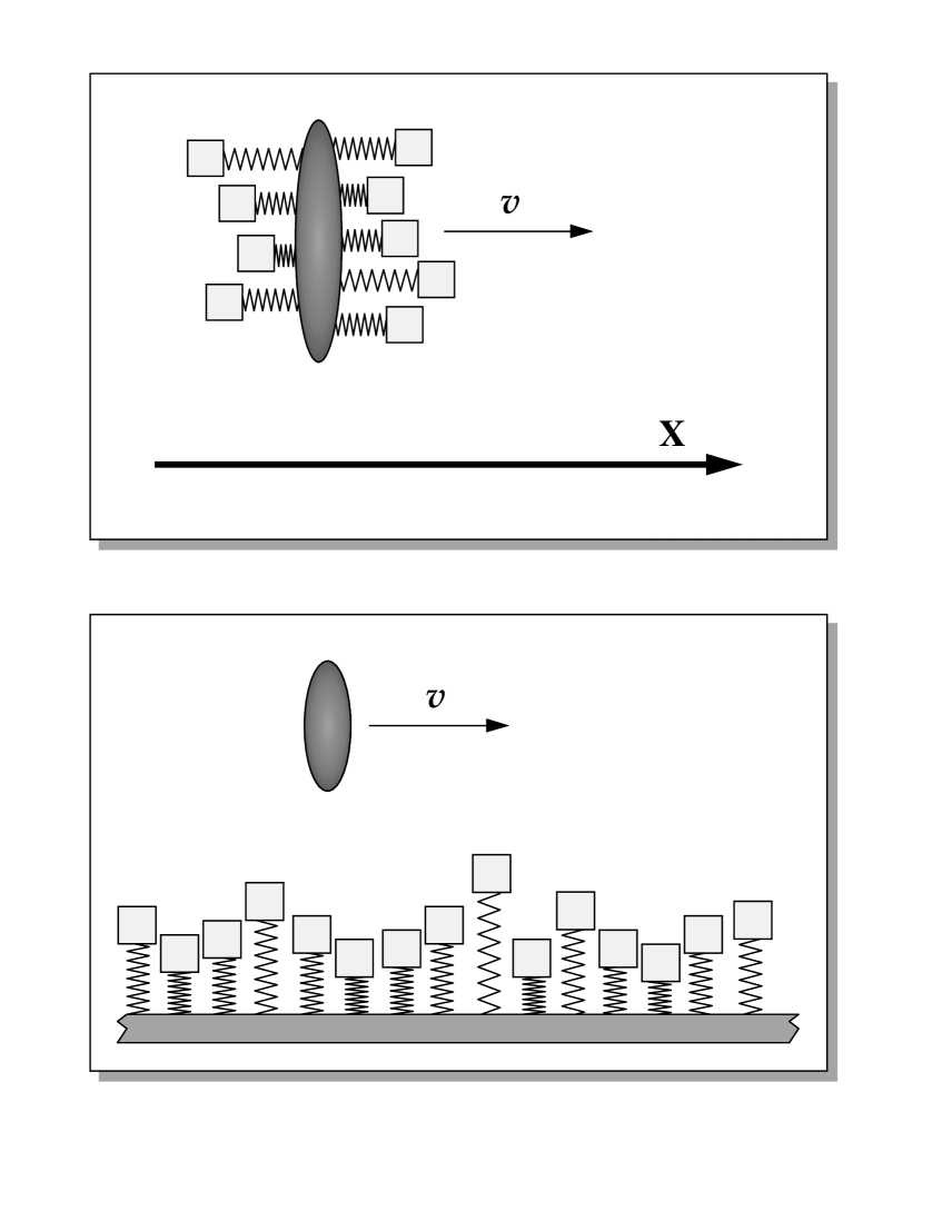
FIG. 1.: Illustration of the BM model (top drawing), versus the DLD model (lower drawing). Note that in the first case a counter term has been incorporated as in (3.13)

Looking at the figure it is apparent that the natural application of the BM model is for the description of the dynamics of a composite particle, with many internal degrees of freedom. This interpretation is due to Gross Ref.[3], who suggested to apply such models for the analysis of heavy-ion collisions. The bath according to this interpretation is “internal”, carried by the particle, rather than “external”.

The interaction Hamiltonian (2.8) may also describe the interaction with some “external” bath that consists of extended field modes. For example, the electron-photon interaction and the electron-phonon interaction may be cast into the form of (2.8), with $u_{\alpha}(x)=\cos(\omega_{\alpha}/c\cdot x),\ \sin(\omega_{\alpha}/c\cdot x)$ , where $c$ is either the speed of light or the speed of sound. In the long wavelength limit this interaction resembles the BM-model rather than the DLD-model. With minor modifications, also these models may be treated within the framework of our “unified” treatment (Appendix A).

Finally, we re-emphasize that in general, the DLD model as well as the BM model may be used on a phenomenological basis for the description of dissipation in mesoscopic quantum devices. This point of view will be discussed further later on (Sec.VI(B) in particular).

III Derivation of Langevin Equation

A The Reduced Equation of motion

The quantal state of the particle may be represented by Wigner function $\rho(R,P)$.  The time evolution of Wigner function corresponds to that of classical distribution in phase-space. In this section we consider a ‘classical treatment of the dynamics’. The latter term implies that the system is considered to be classical, ($\hbar_{system}\rightarrow 0$), while the bath gets full quantum mechanical treatment. The limit $\hbar_{bath}\rightarrow 0$ is not taken. The equations of motion of classical points that form a distribution in phase-space are $\dot{x}=p$ and

$$\dot{p}=-V^{\prime}(x)+{\cal F}_{bath}\ \ ,\ \ \ \ \ {\cal F}_{bath}=\sum_{\alpha}c_{\alpha}Q_{\alpha}(t)u^{\prime}_{\alpha}(x)\ \ \ \ .$$ (3.1)

The variables $Q_{\alpha}(t)$ satisfy the equation

$$m_{\alpha}\ddot{Q}_{\alpha}(t)+m_{\alpha}\omega^{2}_{\alpha}Q_{\alpha}(t)=c_{\alpha}u_{\alpha}(x)$$ (3.2)

which can be solved explicitly, namely,

$$Q_{\alpha}(t)=Q_{\alpha}(0)\cos(\omega_{\alpha}t)+\frac{P_{\alpha}(0)}{m_{\alpha}\omega_{\alpha}}\sin(\omega_{\alpha}t)+\int_{0}^{t}dt^{\prime}\frac{c_{\alpha}}{m_{\alpha}\omega_{\alpha}}\sin(\omega_{\alpha}(t-t^{\prime}))u_{\alpha}(x(t^{\prime}))\ .$$ (3.3)

Substitution of the latter expression into (3.1) yields

$${\cal F}_{bath}={\cal F}_{retarded}+{\cal F}_{noise}$$ (3.4)

with

$${\cal F}_{retarded}=\int_{0}^{t}dt^{\prime}\ 2\alpha(t{-}t^{\prime})\ w^{\prime}(x(t){-}x(t^{\prime}))\ \ \ \ .$$ (3.5)

The response kernel $\alpha(\tau)$ is defined for positive times ($0<\tau$) as follows:

$$\alpha(\tau)=\int^{\infty}_{0}\frac{d\omega}{\pi}J(\omega)\sin(\omega\tau)=-\frac{d}{d\tau}\int^{\infty}_{0}\frac{d\omega}{\pi}\frac{J(\omega)}{\omega}\cos(\omega\tau)\ \ \ \ .$$ (3.6)

In order to make further progress, a specification of the initial state of the system plus the bath is needed. We shall assume that initially (at time $t=0$) the system is prepared in some arbitrary quantal state while the bath oscillators are in thermal canonical equilibrium with some reciprocal temperature $\beta$. The Wigner function representation of the probability density matrix is then (see App. A of Ref.[22]):

$$\rho_{t=0}(R,P;Q_{\alpha},P_{\alpha})=\rho_{t=0}(R,P)\cdot\prod_{\alpha}\rho_{eq}(Q_{\alpha},P_{\alpha})$$ (3.7)

where

$$\rho_{eq}(Q_{\alpha},P_{\alpha})=\ \frac{1}{\frac{1}{2}\coth(\frac{1}{2}\hbar\beta\omega_{\alpha})}\cdot\exp\left[-\beta\left(\frac{\tanh(\frac{1}{2}\hbar\beta\omega_{\alpha})}{(\frac{1}{2}\hbar\beta\omega_{\alpha})}\right)\left(\frac{P^{2}_{\alpha}}{2m_{\alpha}}+\frac{1}{2}m_{\alpha}\omega^{2}_{\alpha}Q^{2}_{\alpha}\right)\right]\ \ .$$ (3.8)

Using (3.8) one obtains the expectation values

$$\langle\frac{P_{\alpha}(0)^{2}}{2m_{\alpha}}\rangle\ \ =\ \ \langle\frac{1}{2}m_{\alpha}\omega^{2}_{\alpha}Q_{\alpha}(0)^{2}\rangle\ \ =\ \ \frac{1}{4}\hbar\omega_{\alpha}\coth(\frac{1}{2}\hbar\beta\omega_{\alpha})\ \ \ \ .$$ (3.9)

Hence it is easily found that $\langle{\cal F}_{noise}(t)\rangle=0$ while

$$\langle{\cal F}_{noise}(t){\cal F}_{noise^{\prime}}(t^{\prime})\rangle\ =\ \ -\sum_{\alpha}c_{\alpha}^{2}\langle Q_{\alpha}(0)^{2}\rangle\cos(\omega_{\alpha}(t{-}t^{\prime}))u_{\alpha}^{\prime}(x)u_{\alpha}^{\prime}(x^{\prime})\ \ \ \ .$$ (3.10)

Thus, one identifies that the noise term is characterized by the autocorrelation function (2.4) with

$$\phi(t-t^{\prime})=\int^{\infty}_{0}\frac{d\omega}{\pi}J(\omega)\ \hbar\coth(\frac{1}{2}\hbar\beta\omega)\ \cos[\omega(t{-}t^{\prime})]$$ (3.11)

The Langevin equation (3.1) together with (3.4)-(3.6) and (3.11) constitutes an exact and complete description of the reduced dynamical behavior of the system, as long as the system is considered to be classical in nature.

B Langevin Equation in the Absence of Disorder

For the BM model $u_{\alpha}(x)=x$. The derivation of Langevin equation (2.1) leads to ${\cal F}_{noise}$ that satisfies (2.2). The latter may be interpreted as a special case of (2.3), provided equation (2.5) for $w(r)$ is used. However, in the expression for the retarded force (3.5), $w^{\prime}(x(t){-}x(t^{\prime}))$ is replaced by $x(t^{\prime})$, rather than by $-(x(t){-}x(t^{\prime}))$. The physical significance of this minor difference is discussed below. In the equation for the retarded force (3.5) one may extend the integration over $t^{\prime}$ to infinity, provided $\alpha(\tau)$ is replaced by $\tilde{\alpha}(\tau)=\alpha(\tau)\Theta(\tau)$, where $\Theta(\tau)$ is the step function. In turn, this kernel may be written as a sum of three terms, namely $\tilde{\alpha}(\tau)=\alpha_{0}(\tau)+\alpha(\tau)+\alpha_{m}(\tau)$ . The kernel $\alpha(\tau)$ is the asymmetric continuation of $\tilde{\alpha}(\tau)$ to the domain $\tau<0$, while $\alpha_{0}(\tau)+\alpha_{m}(\tau)$ is the symmetric continuation. The latter is split into $\alpha_{0}(\tau)$ which is a delta function, and $\alpha_{m}(\tau)$ which satisfies $\int_{-\infty}^{\infty}\alpha_{m}(\tau)d\tau=0$. Consequently, the retarded force, for the BM model, may be written as the sum:

$${\cal F}_{retarded}\ =\ {\cal F}_{switching}+{\cal F}_{\Delta potential}+{\cal F}_{friction}+{\cal F}_{\Delta mass}$$ (3.12)

where ${\cal F}_{switching}\approx-k_{0}\cdot\delta(t)\cdot x(t)$, and ${\cal F}_{\Delta potential}\approx+\Delta k\cdot x(t)$, and ${\cal F}_{friction}\approx-\eta_{eff}\cdot\dot{x}(t)$, and ${\cal F}_{\Delta mass}\approx-\Delta m\cdot\ddot{x}(t)$, with $k_{0}=\eta_{eff}=\lim_{\omega\rightarrow 0}\frac{J(\omega)}{\omega}$, and $\Delta k=\frac{2}{\pi}\int_{0}^{\infty}\frac{J(\omega)}{\omega}d\omega$, and $\Delta m=-\int_{0}^{\infty}\alpha(\tau)\ \tau^{2}\ d\tau$. It has been assumed that $\alpha(\tau)$ has short range duration $\tau_{c}$, much shorter than the physically relevant time scales of the dynamics. This assumption is not true in general, and the consequences will be discussed later in the next section.

The switching impulse act on the particle if it starts its trajectory at a point $x\neq 0$. This term originates due to the fact that the initial preparation is such that the bath is in thermal equilibrium provided $x=0$. The $\Delta potential$ force may be avoided if we care to include in the BM Hamiltonian the proper “counter term”. Namely:

$${\cal H}_{bath}+{\cal H}_{int}\ \ \ \rightarrow\ \ \ \sum_{\alpha}\left(\frac{P_{\alpha}^{2}}{2m_{\alpha}}+\frac{1}{2}m\omega_{\alpha}^{2}(Q_{\alpha}-\frac{c_{\alpha}}{m_{\alpha}\omega_{\alpha}^{2}}x)^{2}\right)$$ (3.13)

This expression is manifestly invariant under space translations. Sanchez-Canizares and Sols have further considered this issue [25].

C Langevin Equation for Disordered Environment

We turn back to the DLD model with ${\cal F}_{retarded}$ as found in equation (3.5). Here, performing similar treatment, neither ${\cal F}_{switching}$ nor ${\cal F}_{\Delta potential}$ are encountered. Formally, this is due to the fact that the difference $-(x(t){-}x(t^{\prime}))$ appears in (3.5), rather than $x(t^{\prime})$ by itself. Physically, this is due to the inherent homogeneity of the interaction with the environment (2.8). As for ${\cal F}_{friction}$ and ${\cal F}_{\Delta mass}$, here one obtains

$${\cal F}_{friction}(v)\ =\ \int_{-\infty}^{\infty}\alpha(\tau)\ w^{\prime}(v\tau)\ d\tau$$ (3.14)

$$\Delta m\ =\ \int_{0}^{\infty}\alpha(\tau)\ w^{\prime\prime}(v\tau)\ \tau^{2}\ d\tau$$ (3.15)

If $\alpha(\tau)$ has short range duration $\tau_{c}$, and if furthermore the velocity of the particle is not too high ($v\cdot\tau_{c}\ll\ell$), then, using $w^{\prime}(0)=0$ and $w^{\prime\prime}(0)=-1$, the above expressions reduce to those that follow equation (3.12). If $\alpha(\tau)$ is not short range, to be discussed below, then the retarded force in the BM model is characterized by long range memory for the dynamics. The approximation that has been used in the preceding subsection is no longer valid, and infinities are encountered in the computations of the constants there. In general, these annoying features are not shared by the DLD model ((3.14) with (2.6)), since a finite cutoff $\tau_{\ell}=\ell/v$ exists, where the microscopic length scale $\ell$ characterizes the interaction range with the scatterers.

IV Ohmic and Non-Ohmic Baths

In order to make further progress, a specification of the spectral function $J(\omega)$ is required. This function, defined in (2.11), characterizes the distribution of the bath-oscillators with respect to their frequencies. Following CL we assume it to be of the form

$$J(\omega)\ =\ \eta\omega^{s}\ G(\omega/\omega_{c}).\ 0<s<1$$ for “subohmic” bath (4.1)

for “ohmic” bath $$s=1$$ (4.2)

for “superohmic” bath $$1<s$$ (4.3)

Here the exponent $s$ characterize the singular behavior of $J(\omega)$ in the vicinity of $\omega=0$, while $G$ denotes a smooth cutoff function. The latter satisfies $G(0)=1$. Moreover, it is assumed that $G(|\omega|)$ is analytic for real frequencies. For example, $G$ may be chosen to be either Lorentzian or Gaussian. The latter possibility will be adopted from now on. The commonly used Exponential cutoff $exp(-\omega/\omega_{c})$ will not be used since it does not satisfies the mentioned requirements. Exponential cutoff results in singular behavior that corresponds to the exponents $s,(s+1),(s+2),...$ rather than “pure” singular behavior that corresponds to $s$ alone. The asymptotic behavior of both $\alpha(\tau)$ and $\phi(\tau)$ is dictated by the singularity of $J(\omega)$ at $\omega=0$. The physical significance of $s$ is further discussed in App.A and in Sec.VI(B).

A Expressions for the Kernels

In order to display explicit expressions for both $\alpha(\tau)$ and $\phi(\tau)$, it is useful to define the following function:

$$G_{s}(\tau)\ \equiv\ \int_{0}^{\infty}\frac{d\omega}{\pi}\ \omega^{s-1}\ \mbox{e}^{-\frac{1}{2}(\frac{\omega}{\omega_{c}})^{2}}\ \cos(\omega\tau)$$ (4.4)

For $s=1$ this function is a normalized Gaussian. For odd $s$ one obtains

$$G_{1{+}2n}(\tau)\ =\ (-1)^{n}\cdot\frac{d^{2n}}{d\tau^{2n}}\left[\frac{\omega_{c}}{\sqrt{2\pi}}\mbox{e}^{-\frac{1}{2}(\omega_{c}\tau)^{2}}\right]\ \ \ \ \ \mbox{[n is integer]}$$ (4.5)

For general $s$ it starts at $\tau=0$ positive

$$G_{s}(0)\ =\ \frac{1}{2\pi}\ 2^{s/2}\ \Gamma(\frac{s}{2})\ \omega_{c}^{s}$$ (4.6)

and cross the $zero$ value $[(s+1)/2]$ times (now we consider $s\neq$ odd number, possibly non-integer). The short range oscillatory behavior dies out on a time scale of the order $\tau_{c}=\omega_{c}^{-1}$. For larger times a power-law decay is found:

$$G_{s}(\tau)=\left(\frac{1}{\pi}\cos(\frac{\pi}{2}s)\Gamma(s)\right)\cdot\frac{1}{\tau^{s}}\ \ \ \ \ \ \mbox{[tail for $s\neq$ odd]}$$ (4.7)

The total algebraic “area” under $G_{s}(\tau)$ is infinite for $0<s<1$, finite for $s=1$, and zero for $1<s$. Representative plots of $G_{s}(\tau)$ are displayed in Fig.2.

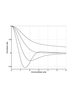
FIG. 2.: Plots of $G_{s}(\tau)$ for $s=0.5$, $s=1$, $s=2$ and $s=4$. The plots are easily distinguished by referring to their description in the text.

For the spectral function $J(\omega)$ as in (4.1), with Gaussian cutoff, the kernel $\alpha(\tau)$ is

$$\alpha(\tau)\ =\ -\eta\ \frac{d}{d\tau}G_{s}(\tau)$$ (4.8)

Also $\phi(\tau)$ can be expressed in terms of $G_{s}(\tau)$ in both cases of “high” and “low” temperatures. In the first case it is assumed that $\hbar\beta$ (that has dimensions of time) is much shorter than any dynamical time scale. One may use then the approximation

$$\phi(\tau)\ =\ 2\frac{\eta}{\beta}\ G_{s}(\tau)\ \ \ \ \ \ \ \mbox{[``high'' temperatures]}.$$ (4.9)

Else, if $\hbar\beta$ is long, one obtains

$$\phi(\tau)\ =\ \frac{2}{\pi}\Gamma(s{+}1)\zeta(s{+}1)\cdot\frac{\eta}{\hbar^{s}}\left(\frac{1}{\beta}\right)^{s{+}1}\ +\ \hbar\eta G_{s{+}1}(\tau)\ \ \ \ \mbox{[``low'' temperatures]},$$ (4.10)

where $\zeta(s)$ is Riemann Zeta function (sum over $1/n^{s}$). The notion “low temperatures” means here $\tau<\hbar\beta$. The temperature-dependent constant term results from the integration $\int_{0}^{\infty}\frac{d\omega}{\pi}J(\omega)\hbar[\coth(\frac{1}{2}\hbar\beta\omega){-}1]$. From now on we shall use the notions of “high” and “low” temperatures in the sense of the above approximations.

B Expressions for Friction and Effective Mass

We turn back to the computation of the terms in (3.12). For the $\Delta potential$ term the result is always finite

$$\Delta k\ =\ \frac{1}{\pi}2^{s/2}\ \Gamma(\frac{s}{2})\ \eta\omega_{c}^{s}\ \ \ \ \mbox{[switching impulse in BM model]}\ \ .$$ (4.11)

For the $friction$ one obtains a finite, non-zero result, ($\eta_{eff}=\eta$) only in the case of an ohmic bath ($s=1$). For subohmic bath ($0<s<1$) the friction is infinite, while for superohmic bath ($1<s$) the friction is zero. In case of the DLD model finite results are obtained for all cases. Using (3.14) one finds out

$${\cal F}_{friction}(v)\ =\ \eta v\int_{-\infty}^{\infty}d\tau\int_{0}^{\infty}\frac{d\omega}{\pi}\ \omega^{s}\ \mbox{e}^{-\frac{1}{2}(\frac{\omega}{\omega_{c}})^{2}}\ \sin(\omega\tau)\cdot\frac{d}{d\tau}\left[\tau_{\ell}^{2}\ \mbox{e}^{-\frac{1}{2}(\frac{\tau}{\tau_{\ell}})^{2}}\right]\$$ (4.12)

$$\ \ =\ -\frac{2}{\pi}\Gamma(1{+}\frac{s}{2})\ 2^{s/2}\cdot\frac{\tau_{\ell}^{3}}{(\tau_{c}^{2}+\tau_{\ell}^{2})^{1+\frac{s}{2}}}\cdot\eta v\ \ \rightarrow\ \ -\frac{2}{\pi}\Gamma(1{+}\frac{s}{2})\ 2^{s/2}\cdot\ell^{1-s}\cdot\eta v^{s}\$$ (4.13)

Above, the notation $\tau_{\ell}=\ell/v$ has been used. In the last step the limit $\omega_{c}\rightarrow\infty$ has been taken since it leads to a finite, non-zero result. Note that the cutoff frequency $\omega_{c}$ is not relevant physically as long as $v\ll\ell\cdot\omega_{c}$. The above computation clarifies the significance of the various time scales. Formally, the BM model constitutes a special case with $\tau_{\ell}=\infty$. For $s=1$, the so called “ohmic” case, one obtains ${\cal F}_{friction}=-\eta v$. This result holds in the case of the DLD model as well as in the case of the BM model. In the latter case, for $s<1$ or for $1<s$, the friction force is either infinite or zero respectively. This is due to a long range memory effect. The cutoff frequency $\omega_{c}$, by itself, does not prevent this feature. Finite results for the components of retarded force in the BM model (3.12) may be obtained only for bounded systems, where $x(t)$ explores only a finite portion of the space. The calculation above (4.12) manifests the fact that a finite result, in case of unbounded system, may be obtained if a physical cutoff $\tau_{\ell}$ is introduced. Such arise naturally in case of the DLD model.

Similar picture emerges upon calculation of the effective mass. For the BM model, a finite result is obtained in case of an ohmic bath ($s=1$).

$$\Delta m\ =\ \int_{0}^{\infty}\eta\frac{d}{d\tau}\left[\frac{\omega_{c}}{\sqrt{2\pi}}\mbox{e}^{-\frac{1}{2}(\omega_{c}\tau)^{2}}\right]\cdot\tau^{2}\cdot d\tau\ =\ -\sqrt{\frac{2}{\pi}}\ \frac{\eta}{\omega_{c}}\ \ \ \ \ \ \ \ \ \ \ \ \ \mbox{for $s=1$}$$ (4.14)

Also for $2<s$, the power law tail of $\alpha(\tau)$ decays sufficiently fast to guarantee a finite result:

$$\Delta m\ =\ \frac{1}{2\pi}\ 2^{s/2}\ \Gamma(\frac{s}{2}-1)\cdot\eta\omega_{c}^{s-2}\ \ \ \ \ \ \ \ \ \ \ \ \ \mbox{for $2<s$}\ \ \ \ .$$ (4.15)

For $0<s<2$ ($s\neq 1$), the effective mass is infinite. In order to obtain a finite result we should turn to the DLD model (3.14). Here, as in the case of friction calculation, the spectral cutoff $\omega_{c}$ is not important, and will be taken to infinity. Thus the integration may be performed using the asymptotic expression for $\alpha(\tau)$. Substitution of (2.6), (4.8) and (4.7) yields

$$\Delta m\ \ = \ \ \frac{\eta}{\pi}\cos(\frac{\pi}{2}s)\Gamma(s)\int_{0}^{\infty}\frac{-s}{\tau^{s{+}1}}\frac{d^{2}}{d\tau^{2}}\left[\tau_{\ell}^{2}\ \mbox{e}^{-\frac{1}{2}(\frac{\tau}{\tau_{\ell}})^{2}}\right]\ \tau^{2}\ d\tau$$ (4.16)

$$= -\frac{s(s-1)}{\pi}\cos(\frac{\pi}{2}s)\Gamma(s)\Gamma(1{-}\frac{s}{2})\ 2^{-s/2}\cdot\eta\tau_{\ell}^{2-s}\ \sim\ -\frac{\eta}{v^{s{-}2}}\ \ \ \ \mbox{[for $0{<}s{<}2$]}$$ (4.17)

For the special case $s=1$ one obtains $\Delta m=0$ which is consistent with (4.14) in the limit $\omega_{c}\rightarrow\infty$. For $s\rightarrow 2$ a negative infinite value is obtained, while from (4.15) a positive infinite value is obtained. In order to describe correctly the crossover at $s=2$, one should introduce finite cutoff $\omega_{c}$ as well as finite $\tau_{\ell}$. The calculation will not be carried here.

V Propagator For Non Dynamical Environment

In this section we shall develop a path-integral expression for the propagator of a particle that interacts either with static (quenched) or noisy environment. First we develop a classical expression, and then we generalize to the quantal regime.

A Classical Derivation

We refer to the dynamics generated by the Hamiltonian (2.7). The classical Liouville propagator, over infinitesimal time $d\tau$, and for definite realization of ${\cal U}$ is:

$${\cal K}(R_{2},P_{2}|R_{1},P_{1})=2\pi\delta\left((P_{2}{-}P_{1})+(\frac{\partial V}{\partial R}{+}\frac{\partial{\cal U}}{\partial R})d\tau\right)\cdot\delta\left((R_{2}{-}R_{1})-\frac{P}{m}d\tau\right)$$ (5.1)

It is more convenient to write an expression for the propagator of the Fourier transformed probability function ($\rho(R,P)\rightarrow\rho(R,r)$), namely,

$${\cal K}(R_{2},r_{2}|R_{1},r_{1})=(\frac{m}{2\pi\hbar d\tau})\cdot\exp\left[\frac{1}{\hbar}\left(im(\frac{R_{2}{-}R_{1}}{d\tau})(r_{2}{-}r_{1})\ -\ i(\frac{\partial V}{\partial R}{+}\frac{\partial{\cal U}}{\partial R})(\frac{r_{2}{+}r_{1}}{2})d\tau\right)\right]$$ (5.2)

Here a dummy parameter $\hbar$ has been inserted. Its value does not have any effect here. However, later comparison to the quantum mechanical version will be more transparent. For finite time, the convolved propagator may be written as a functional integral:

$${\cal K}(R,r|R_{0},r_{0})=\int_{R(0)}^{R}\int_{r(0)}^{r}{\cal D}R{\cal D}r\ \exp\left[\frac{1}{\hbar}\left(im\int_{0}^{t}d\tau\dot{R}\dot{r}\ -\ i\int_{0}^{t}d\tau\frac{\partial V}{\partial R}\cdot r(\tau)\right.\right.-\left.\left.i\int_{0}^{t}d\tau\frac{\partial{\cal U}}{\partial R}\cdot r(\tau)\right)\right]$$ (5.3)

Here the measure is

$${\cal D}R\ {\cal D}r\ =\ \ {\left(\frac{m}{2\pi\hbar d\tau}\right)}^{\mbox{\# segments}}\ ...dR_{3}dR_{2}dR_{1}\ ...dr_{3}dr_{2}dr_{1}$$ (5.4)

and the restrictions at the endpoints are $R(0)\!=\!R_{0}$, $r(0)\!=\!r_{0}$ and $R(t)\!=\!R$, $r(t)\!=\!r$. It is now possible to average over realizations of ${\cal U}$, using the well known Gaussian identity

$$\langle\mbox{e}^{i\int d\tau k(\tau)z(\tau)}\rangle_{z}\ =\ \ e^{-\frac{1}{2}\int d\tau d\tau^{\prime}\langle z(\tau)z(\tau^{\prime})\rangle k(\tau)k(\tau^{\prime})}$$ (5.5)

One obtains

$${\cal K}(R,r|R_{0},r_{0})=\int_{R(0)=R_{0}}^{R}\int_{r(0)=r_{0}}^{r}{\cal D}R{\cal D}r\ \ \mbox{e}^{i\frac{1}{\hbar}S_{eff}[R,r]}\ \ \mbox{e}^{-\frac{1}{\hbar^{2}}S_{N}[R,r]}$$ (5.6)

where

$$S_{eff}[R,r]=S_{free}[R,r]-\int_{0}^{t}d\tau\frac{\partial V}{\partial R}\cdot r(\tau)\ \ \ \ \ \ \mbox{[classical]}$$ (5.7)

and

$$S_{N}[R,r]=\frac{1}{2}\int_{0}^{t}\int_{0}^{t}d\tau_{1}d\tau_{2}\ [-\phi^{\prime\prime}(R(\tau_{2}){-}R(\tau_{1}),\tau_{2}{-}\tau_{1})]\ r(\tau_{2})r(\tau_{1})$$ (5.8)

The free part of the effective action, for use in (5.6), is $S_{free}[R,r]=m\int_{0}^{t}d\tau\dot{R}\dot{r}$. It may be more convenient to write down the path-integral expression for ${\cal K}(R,P|R_{0},P_{0})$. This expression is obtained by double Fourier transform of ${\cal K}(R,r|R_{0},r_{0})$. The result is

$${\cal K}(R,P|R_{0},P_{0})=\int_{R_{0},P_{0}}^{R,P}\!\!\!{\cal D}R\int{\cal D}r\ \ \mbox{e}^{i\frac{1}{\hbar}S_{eff}[R,r]}\ \ \mbox{e}^{-\frac{1}{\hbar^{2}}S_{N}[R,r]}$$ (5.9)

Here,

$$S_{free}[R,r]=-m\int_{0}^{t}d\tau\ddot{R}{r}\ \ \ \ \ \ \ \mbox{[For use in (\ref{e6_7})]}\ \ \ .$$ (5.10)

Note that the integration ${\cal D}r$ is not restricted at the end-points, whereas the integration ${\cal D}R$ is restricted at the end-points both in $R$ and in $\dot{R}$. The restriction on $\dot{R}$ at the endpoints is implicit, through the dispersion relation $\dot{R}=P/m$.

B Qauntal Derivation

A similar expression may be obtained for the quantal propagator. Again, we refer to the dynamics generated by the Hamiltonian (2.7). The environment may be either “noisy” or “quenched”, where the latter case constitute formally a special case of the former. The expression that will be obtained is a generalization of a result that has been obtained in Ref.[16] for white noise potential.

The Feynman path-integral expression for the propagator of the quantal wave-function is,

$$U(x|x_{0})=\int_{x(0)=x_{0}}^{x}\!\!\!\!{\cal D}x\ \ \mbox{e}^{i\frac{1}{\hbar}\int_{0}^{t}d\tau(\frac{1}{2}m\dot{x}^{2}-V(x)-{\cal U}(x,t))}\ \ \ .$$ (5.11)

The path integral expression for the propagator of the density probability function constitutes summation ${\cal D}x^{\prime}{\cal D}x^{\prime\prime}$ over the pairs of paths $x^{\prime}(\tau)$ and $x^{\prime\prime}(\tau)$. Alternatively, we may use also the coordinates $R=(x^{\prime}{+}x^{\prime\prime})/2$ and $r=(x^{\prime\prime}{-}x^{\prime})$, thus the summation will be ${\cal D}R{\cal D}r$, namely

$${\cal K}(R,r|R_{0},r_{0})=\int_{R_{0}}^{R}{\cal D}R\int_{r_{0}}^{r}{\cal D}r\ \ \mbox{e}^{i\frac{1}{\hbar}S_{eff}[R,r]-i\frac{1}{\hbar}\int_{0}^{t}d\tau({\cal U}(x^{\prime\prime},\tau)-{\cal U}(x^{\prime},\tau))}$$ (5.12)

where

$$S_{eff}[R,r]=S_{free}[R,r]-\int_{0}^{t}d\tau(V(x^{\prime\prime},\tau){-}V(x^{\prime},\tau))$$ (5.13)

It is important to notice that the quantal definition of the measure is identical with the classical one (5.4). In order to perform the average over realizations of ${\cal U}$ using the Gaussian identity (5.5), one may write the last expression as

$${\cal K}(R,r|R_{0},r_{0})=\int_{R_{0}}^{R}\int_{r_{0}}^{r}{\cal D}R{\cal D}r\ e^{i\frac{1}{\hbar}S_{eff}[R,r]-i\frac{1}{\hbar}\int_{0}^{t}d\tau\int_{-\infty}^{\infty}dz(\delta(z{-}x^{\prime\prime})-\delta(z{-}x^{\prime})){\cal U}(z,\tau)}$$ (5.14)

One easily find that the final result may be cast to the form of equation (5.6) or (5.9) with

$$S_{N}[R,r]=\frac{1}{2}\int_{0}^{t}\int_{0}^{t}d\tau_{1}d\tau_{2}\ (\phi(x_{2}^{\prime\prime}{-}x_{1}^{\prime\prime},\tau_{2}{-}\tau_{1})+\phi(x_{2}^{\prime}{-}x_{1}^{\prime},\tau_{2}{-}\tau_{1})-2\phi(x_{2}^{\prime\prime}{-}x_{1}^{\prime},\tau_{2}{-}\tau_{1}))$$ (5.15)

where $x_{i}$ is a short notation for $x(\tau_{i})$.

We are now in position to compare the classical propagator ((5.9) with (5.7)-(5.8)), with the quantal one ((5.9) with (5.7)-(5.8)). In the latter case $\hbar$ is, in general, no longer a “dummy variable”. The exception being the case where the actions are quadratic in the path variables, which is the case with BM model provided $V(x,t)$ is quadratic. The “classical feature” may be characterized as arising from invariance under the scaling transformation of the auxiliary integration-variable $r(\tau)$. In the quantal regime the replacement $\hbar\rightarrow\lambda\hbar$ cannot be compensated by the scaling $r\rightarrow\lambda r$. Note however that the limit $\hbar\rightarrow 0$ is equivalent to taking leading behavior of the actions in the limit $r\rightarrow 0$.

VI Propagator for Dynamical Environment

A Feynman Vernon Formulation

Here we follow closely the notations in Ref.[21]. The path-integral expression for the reduced propagator of the probability density function is of the general form (5.9), with

$$S_{eff}[R,r]=S_{free}[R,r]-\int_{0}^{t}d\tau(V(x^{\prime\prime},\tau){-}V(x^{\prime},\tau))+S_{F}[x^{\prime\prime},x^{\prime}]$$ (6.1)

The expressions for the reduced-action-functionals $S_{F}[x^{\prime},x^{\prime\prime}]$ and $S_{N}[x^{\prime},x^{\prime\prime}]$ in case of BM model, are given in equations (2.13)-(2.14) of the latter reference. In the BM model the interaction is via the dynamical variable $x$, while, in DLD model, the interaction is via $u_{\alpha}(x)$. Thus, in the expressions for the friction functional $S_{F}[x^{\prime},x^{\prime\prime}]$ and for the noise functional $S_{N}[x^{\prime},x^{\prime\prime}]$ one should make the replacements  $x^{\prime}\rightarrow u_{\alpha}(x^{\prime})\ ,\ x^{\prime\prime}\rightarrow u_{\alpha}(x^{\prime\prime})$  , and sum over $\alpha$. Thus one obtains

$$S_{F}[x^{\prime},x^{\prime\prime}]\ =\ \frac{1}{\mbox{density}}\times\int_{0}^{t}\int_{0}^{t}d\tau_{1}d\tau_{2}\ 2\tilde{\alpha}(\tau_{2}{-}\tau_{1})\ \frac{1}{2}\sum_{\alpha}(u_{\alpha}(x_{2}^{\prime\prime}){-}u_{\alpha}(x_{2}^{\prime}))(u_{\alpha}(x_{1}^{\prime\prime}){+}u_{\alpha}(x_{1}^{\prime}))$$ (6.2)

and

$$S_{N}[x^{\prime},x^{\prime\prime}]\ =\ \frac{1}{\mbox{density}}\times\frac{1}{2}\int_{0}^{t}\int_{0}^{t}d\tau_{1}d\tau_{2}\ \phi(\tau_{2}{-}\tau_{1})\ \sum_{\alpha}(u_{\alpha}(x_{2}^{\prime\prime}){-}u_{\alpha}(x_{2}^{\prime}))(u_{\alpha}(x_{1}^{\prime\prime}){-}u_{\alpha}(x_{1}^{\prime}))\ \ \ \ \ \ .$$ (6.3)

Above $\tilde{\alpha}(\tau)\equiv\alpha(\tau)\Theta(\tau)$. These expressions may be simplified using (2.12). The results are

$$S_{F}[x^{\prime},x^{\prime\prime}]=\int_{0}^{t}\int_{0}^{t}d\tau_{1}d\tau_{2}\ 2\tilde{\alpha}(\tau_{2}{-}\tau_{1})\cdot\frac{1}{2}[w(x_{2}^{\prime\prime}{-}x_{1}^{\prime\prime})-w(x_{2}^{\prime}{-}x_{1}^{\prime})+w(x_{2}^{\prime\prime}{-}x_{1}^{\prime})-w(x_{2}^{\prime}{-}x_{1}^{\prime\prime})]$$ (6.4)

and

$$S_{N}[x^{\prime},x^{\prime\prime}]=\frac{1}{2}\int_{0}^{t}\int_{0}^{t}d\tau_{1}d\tau_{2}\ \phi(\tau_{2}{-}\tau_{1})\ [w(x_{2}^{\prime\prime}{-}x_{1}^{\prime\prime})+w(x_{2}^{\prime}{-}x_{1}^{\prime})-2w(x_{2}^{\prime\prime}{-}x_{1}^{\prime})]$$ (6.5)

In the next paragraph we discuss further the physical significance of the functional $S_{F}[x^{\prime},x^{\prime\prime}]$.

For the BM model it has been noted before that in practice one could substitute (2.5). Thus

$$S_{F}[x^{\prime},x^{\prime\prime}]=\int_{0}^{t}\int_{0}^{t}d\tau_{1}d\tau_{2}\ 2\tilde{\alpha}(\tau_{2}{-}\tau_{1})\ r(\tau_{2})\cdot(R(\tau_{1})-R(\tau_{2}))\ \ \ \ .$$ (6.6)

However, the formally “correct” expression is somewhat different (Ref.[21] equation (2.13)). Namely, the integrand in the above equation is with $r(\tau_{2})R(\tau_{1})$, rather than $r(\tau_{2})(R(\tau_{1}){-}R(\tau_{2}))$. One may say that the BM reduced-action functional includes an additional term. It is not difficult to demonstrate that the latter can be split into two terms that corresponds exactly to ${\cal F}_{\Delta potential}$ and to ${\cal F}_{switching}$ discussed in Sec.III(B). The $\Delta potential$ term may be absorbed in the definition of $V(x)$, while the $switching$ term, which is $-\Delta k\ r(0)R(0)$, may be factored out of the path integral expression (see Ref.[21] equation (2.34)). It has the effect of operating on the initial probability function with an impulse that acts on the particle if it starts its trajectory in a point $x\neq 0$. This term originates due to the fact that the initial preparation is such that the bath is in thermal equilibrium provided $x=0$. Both the “switching” term and the additional effective potential, are absent in DLD model. This obvious results stems from the assumed inherent homogeneity of the environment. We turn now to the general expression (6.4). Again, as in Sec.III(B), it is convenient to express $\tilde{\alpha}(\tau)$ as a sum of its symmetric, and antisymmetric continuations. Here we focus on the resultant friction functional, which is

$$S_{F}|_{friction}\ =\ \ \int_{0}^{t}\int_{0}^{t}d\tau_{1}d\tau_{2}\ \alpha(\tau_{2}{-}\tau_{1})\ w(x^{\prime\prime}(\tau_{2}){-}x^{\prime}(\tau_{1}))$$ (6.7)

For Ohmic bath one obtains

$$S_{F}\ =\ \eta\int_{0}^{t}d\tau\ w^{\prime}(r(\tau))\ \dot{R}(\tau)\ \ \ \rightarrow\ \ \ -\eta\int_{0}^{t}d\tau\ r(\tau)\ \dot{R}(\tau)$$ (6.8)

where in the last stage we indicated the classical limit. Note that the classical expression for $S_{F}$ can be easily derived. For this one should include the friction force in the derivation of Sec.V(A).

B Derivation for Generic Bath

A totally different derivation of the path integral expression for the propagator is possible in the general case of weak coupling to thermal, possibly chaotic bath. This derivation, in case of linear coupling, has been introduce already by FV Ref.[5]. The case of general, nonlinear coupling, has been considered by Möhring and Smilansky Ref.[6]. Here we shall take a step further, and demonstrate that under “normal” circumstances, it will reduce to an ohmic DLD model. We consider a bath Hamiltonian of the general form:

$${\cal H}_{bath}+{\cal H}_{int}\ =\ \sum_{n}|n\rangle E_{n}\langle n|\ +\ \sum_{nm}|m\rangle{\cal U}_{mn}(x)\langle n|\ \ \ \ ,$$ (6.9)

where $|n\rangle$ and $E_{n}$ are the eigenstates and eigenenergies of the bath Hamiltonian in the absence of the coupling. This Hamiltonian depends on $x$, the system variable, as a parameter. However, once the full Hamiltonian (2.10) is considered, $x$ becomes a dynamical variable. The so called Influence Functional, in our notations is (by definition):

$$\mbox{e}^{i(S_{F}+iS_{N})}\ =\ \sum_{nm}p_{n}\ U_{mn}[x^{\prime\prime}(\tau)]\ U_{mn}^{\star}[x^{\prime}(\tau)]\ \ \ \ ,$$ (6.10)

Units with $\hbar=1$ are used here. $U[x(\tau)]$ is the evolution operator of the bath, in the presence of the “driving force” $x(\tau)$. The bath is assumed to be in canonical thermal equilibrium. The probability of the $n$-th eigenstate is $p_{n}\propto e^{-\beta E_{n}}$. Using leading order perturbation theory one obtains

$$U_{mn}[x(\tau)]\ \approx\ -i\int_{0}^{t}d\tau\ {\cal U}_{mn}(x(\tau))\ \mbox{e}^{i(E_{m}-E_{n})\tau}\ \ \ \ \ \ \mbox{for $m\neq n$}\ \ .$$ (6.11)

Similar expression holds for $m{=}n$ (see Ref.[6]). Substitution into (6.10) yields:

$$(iS_{F}-S_{N})\ \ =\ \ \sum_{nm}p_{n}\ \left[\int_{0}^{t}\int_{0}^{t}d\tau_{2}d\tau_{1}\ {\cal U}_{mn}(x_{2}^{\prime\prime}){\cal U}_{mn}^{\star}(x_{1}^{\prime})\ \mbox{e}^{i(E_{m}-E_{n})(\tau_{2}-\tau_{1})}\ \ \ \ \ \ \ \right.\ \ \ \ \ \ \ \ \ \ \ \ \ \ \ \ \ \ \ \ \ \ \ \$$ (6.12)

$$\left.-\int_{0}^{t}\int_{0}^{\tau_{2}}d\tau_{2}d\tau_{1}\left({\cal U}_{mn}(x_{2}^{\prime\prime}){\cal U}_{mn}(x_{1}^{\prime\prime})\ \mbox{e}^{-i(E_{m}{-}E_{n})(\tau_{2}{-}\tau_{1})}-{\cal U}_{mn}^{\star}(x_{2}^{\prime}){\cal U}_{mn}^{\star}(x_{1}^{\prime})\ \mbox{e}^{i(E_{m}{-}E_{n})(\tau_{2}{-}\tau_{1})}\right)\right]$$ (6.13)

Now we take a further assumption which will reduce the resultant expression for $S_{F}$ and $S_{N}$ to the form of (6.4) and (6.5) respectively. The matrix elements ${\cal U}_{mn}$ are assumed to be real, while their dependence on $x$ is assumed to be characterized by the function

$$\pi\ \sum_{mn}\ (p_{n}-p_{m})\ {\cal U}_{mn}(x_{2}){\cal U}_{mn}(x_{1})\ \delta(\omega-(E_{m}{-}E_{n}))\ \ =\ \ w(x_{2}{-}x_{1})\cdot J(\omega)\ \ \ \ \ .$$ (6.14)

The reduction of (6.12) to (6.4) and (6.5) is easily verified via algebraic manipulation, using $\Im[\sum_{nm}p_{n}\{..\}]{=}\sum_{nm}(p_{n}{-}p_{m})\{..\}$ and $\Re[\sum_{nm}p_{n}\{..\}]{=}\sum_{nm}\coth(\frac{1}{2}\beta\omega)(p_{n}{-}p_{m})\{..\}$ where $\coth(\frac{1}{2}\beta\omega){=}(p_{n}{+}p_{m})/(p_{n}{-}p_{m})$. Thus, for general nonlinear coupling, DLD model constitutes an equivalent representation for the bath, as far as the reduced dynamics of the system is concerned. For the particular case of the weak linear coupling, there is further reduction to the BM model, with

$$J(\omega)\ =\ \pi\sum_{n,m}\ (p_{n}-p_{m})\ |Q_{mn}|^{2}\ \delta(\omega-(E_{m}{-}E_{n}))$$ (6.15)

In the above expression $Q$ denotes the collective bath degree of freedom via which the interaction takes place, namely, in (6.9) one should substitute ${\cal U}(x)=Q\cdot x$. The bath variable $Q$ may be some complicated nonlinear combination of many elementary bath degrees of freedom. For both, the DLD model and the BM model, the expression for $J(\omega)$ , may be cast into the form

$$J(\omega)\ =\ \ \frac{\pi}{\beta Z(\beta)}\ (1-\mbox{e}^{-\beta\omega})\ \sigma(\omega)^{2}\ K(\omega)$$ (6.16)

where $Z(\beta)$ is the partition function, $\sigma(\omega)$ is the standard deviation of the off-diagonal matrix elements ($\omega$ being the offset), and $K(\omega)$ is the density-density autocorrelation function of the spectrum $\{E_{n}\}$, appropriately averaged over the relevant energy scale. The latter is related, for small energy differences, to the level spacing distribution. However, for any practical use, one should ignore the effect of level spacing statistics on $J(\omega)$, since it corresponds to non-physically very long times. Thus, the generic behavior of $J(\omega)$, for physically-relevant small $\omega$, is expected to be $linear$. This leads to the conclusion that under “normal” circumstances the ohmic DLD model is good representation for the dissipation process. This conclusion does not hold if strong coupling to a chaotic bath is considered. In the latter case Zener transitions may dominate the dissipation process [9, 10]. We do not know whether the Influence Functional (6.10) for that case can be reduced to a form that resembles that of the DLD model.

C Loss of Quantal Interference

The suppression of quantal interference is an important issue in both semiclassical and mesoscopic physics. It may arise that the quantum mechanical propagator may be expressed as a sum of probabilities to go either via one classical trajectory $x_{a}(\tau)$ or via a different classical trajectory $x_{b}(\tau)$, plus an interference term. The expression for the Influence Functional may be used in order to compute the suppression of the interference due to the interaction with the environment. The interference term is multiplied by a “dephasing” factor $\langle e^{i\varphi}\rangle$, where we follow a notation due to Stern, Aharonov and Imry [18]. In our notations, the dephasing factor is identified with $\exp(-S_{N}[x_{a}(\tau),x_{b}(\tau)])$. We defer further discussion of interference within the framework of FV formalism to the last paragraph of this subsection.

It is enlightening to consider the case of white noise, with $\phi(\tau_{2}{-}\tau_{1})=\nu\delta(\tau_{2}{-}\tau_{1})$. For the BM model one obtains

$$\langle\mbox{e}^{i\varphi}\rangle\ =\ \ \exp\left[-\frac{1}{2}\frac{\nu}{\hbar^{2}}\int_{0}^{t}\ (x_{a}(\tau)-x_{b}(\tau))^{2}\ d\tau\right]\ \ \ \ .$$ (6.17)

Thus, interference is suppressed more effectively if the two interfering paths are better separated. A totally different result is obtained in case of the DLD model. Here we assume that the two interfering paths are well separated with respect to the microscopic scale $\ell$, namely $\ell\ll|x_{a}(\tau){-}x_{b}(\tau)|$ most of the time. It follows that

$$\langle\mbox{e}^{i\varphi}\rangle\ =\ \ \exp\left[-\frac{\nu\ell^{2}}{\hbar^{2}}\cdot t\right]\ \ \ \ .$$ (6.18)

Here, the interference decays exponentially in time, and the actual spatial separation of the paths play no role. Due to the disorder, dephasing events are as effective for small separations as for large separations.

The dephasing of interference in metals due to electromagnetic fluctuations has been discussed by Al’tshuler, Aronov and Khmelnitskii in Ref.[17]. Their results have been re-derived by Stern, Aharonov and Imry [18]. A somewhat simplified derivation is reconstructed in App.A. The strong dimensionality dependence of the dephasing process has been emphasized. This dependence is due to the separation-dependence as in (6.17), and see also (A.6). In case of the DLD model, the local nature of the dephasing process will eliminate this feature.

In order to understand how interference arise from the FV path integral expression (5.9), it is convenient to rewrite it in the following form

$${\cal K}(R,P|R_{0},P_{0})\ \ =\ \ \int_{R_{0},P_{0}}^{R,P}{\cal D}R\ \ {\cal K}[R]\ \ \ \ ,$$ (6.19)

where ${\cal K}[R]$ is a real functional, which is defined by the expression:

$${\cal K}[R]=\int_{unrestricted}\!\!\!\!{\cal D}r\ \ \mbox{e}^{i\frac{1}{\hbar}S_{eff}[R,r]}\ \ \mbox{e}^{-\frac{1}{\hbar^{2}}S_{N}[R,r]}\ \ \ \ \ .$$ (6.20)

If the path integral expression for the evolution operator (5.11) is dominated by a single classical path $x_{a}(\tau)$, then the ${\cal D}R$ integration in (6.19) will be dominated by $R(\tau)=x_{a}(\tau)$. Obviously, in order to obtain a non-vanishing result, the endpoint conditions should be compatible. Turning to the computation of ${\cal K}[R(\tau){=}x_{a}(\tau)]$ via (6.20), one observes that the ${\cal D}r$ integration is dominated by the trivial trajectory $r_{R}(\tau){=}0$. We use the subscript $R$ in order to suggest that in general this trajectory should be $R$-dependent. Indeed, this is the case if two classical trajectories $x_{a}(\tau)$ and $x_{b}(\tau)$ dominate. One should consider then the “interference path” $R(\tau){=}(x_{a}(\tau){+}x_{b}(\tau))/2$, for which the ${\cal D}r$ integration is dominated by the non-trivial paths $r_{R}(\tau){=}\pm(x_{a}(\tau){-}x_{b}(\tau))$. The existence of non-trivial path $r_{R}$ is the fingerprint of interference phenomena. A classical trajectory $R(\tau)$ for which $r_{R}{=}0$ will not be damped, since $S_{N}[R,r_{R}]=0$ then. In contrast, an interference path, for which $r_{R}\neq 0$, is damped, since $0<S_{N}[R,r_{R}]$ in general. However, in Sec.IX, where localization effect is discussed, we shall encounter a vast family of interference trajectories that are not damped by the noise functional. In the latter case, the interference paths are found to be dominant in the computation of the propagator.

Another issue that deserves attention is the interplay of friction and interference. By inspection of (6.7) it is clear that for disordered environment, quantal interference is unaffected by friction. This is true as long as $x_{a}$ and $x_{b}$ are well separated in space. In Sec.VII(B) we shall encounter a related quantal manifestation of this observation.

VII Spreading and Diffusion

The main results of the two last sections are the path integral expression (5.9) for the propagator ${\cal K}(R,P|R_{0},P_{0})$, with the appropriate action functionals $S_{free}$ (5.10), $S_{F}|_{friction}$ (6.7), and $S_{N}$ (6.5). The classical limit of $S_{N}$ is presented in (5.8). For ohmic friction, both the quantal version and its classical limit (6.8) will be further considered and compared. Friction in case of non-ohmic bath has been discussed in Sec.IV, and its quantal analog will not be considered further.

In order to get preliminary insight into the path-integral expression, consider first the case of free particle in “white” noisy environment. Namely, $\phi(\tau{-}\tau^{\prime})=\nu\delta(\tau{-}\tau^{\prime})$, with $\nu=2\eta k_{B}T$ as in 4.9. In the classical case (5.8), one obtains

$$S_{N}[r]=\frac{1}{2}\nu\int_{0}^{t}\ r(\tau)^{2}d\tau\ \ \ .$$ (7.1)

independent of the spatial auto-correlation function $w(r)$. The observation that spatial correlations are of no importance, as long as the noise is uncorrelated in time, is trivial from classical point of view. In the quantum mechanical case, the corresponding expression is

$$S_{N}[r]=\nu\int_{0}^{t}\ (w(0){-}w(r(\tau))\ d\tau\ \ \ .$$ (7.2)

In contrary to classical intuition, spatial correlations may be of importance. However, for the BM model, (2.5), one recovers the classical result.

In the path integral expression (5.9), one may perform the integration ${\cal D}r=...dr_{3}dr_{2}dr_{1}$  . In the absence of $S_{N}$, each integration over $dr_{n}$ results in delta function of velocities, namely $\delta(\dot{R}(\tau_{n+1})-\dot{R}(\tau_{n}))$. In the presence of $S_{N}$, the integration $dr_{n}$ is weighted, and as a result, each $\delta$ function is smeared. The propagator constitutes a convolution of these smeared $\delta$ functions. In particular, both in the classical case and in the BM model, each smeared $\delta$ function is a Gaussian. It is obvious, that both in the classical and in the quantal case, $S_{N}$ leads to stochastic-like spreading. In what follow we want to estimate this spreading.

A Non Disordered Environment

We turn now to estimate the spreading in the absence of disorder, which is the standard BM model. The noise functional is quadratic in the path-variable $r$, and is independent of the path-variable $R$, namely

$$S_{N}[R,r]=\frac{1}{2}\int_{0}^{t}\int_{0}^{t}d\tau_{1}d\tau_{2}\ \phi(\tau_{2}{-}\tau_{1})\ r(\tau)r(\tau^{\prime})$$ (7.3)

Here, an exact treatment is available [21]. One may expand both $S_{free}$ and $S_{N}$ around the so-called classical paths, that are determined by the variation $\delta S_{free}=0$, with the constraints $\delta R{=}\delta r{=}0$ at the endpoints. The Gaussian integration is performed exactly. General expressions may be found in Ref.[21]. The phase space propagator ${\cal K}(R,P|R_{0},P_{0})$ is obtained by double Fourier transform of ${\cal K}(R,r|R_{0},r_{0})$, and obviously results in Gaussian function. In particular, one is interested in the spatial spreading. Setting $P_{0}=0$ and integrating over the final momentum $P$, one obtains

$${\cal K}(R|R_{0})=\frac{1}{2\pi\sqrt{\sigma_{spatial}}}\exp\left[\frac{1}{2}\left(\frac{R{-}R_{0}}{\sigma_{spatial}}\right)^{2}\right]$$ (7.4)

A general expression for the spatial spreading, that applies to any $\phi(\tau)$, may be obtained [21]:

$$\sigma_{spatial}\ =\ \ \frac{1}{m}\ \sqrt{\int_{0}^{t}\int_{0}^{t}\phi(\tau{-}\tau^{\prime})\ r_{c\ell}(\tau)\ r_{c\ell}(\tau^{\prime})\ d\tau d\tau^{\prime}\ }\ \ \ ,$$ (7.5)

where $r_{c\ell}$ solves the linearized classical equation of motion ($m\ddot{r}+\eta\dot{r}=0$) with initial conditions $r(0)=0$ and $\dot{r}(0)=1$. Note that ohmic friction is considered, for which the BM model is well defined. For the simplest case of white noise without friction one obtains $\sigma_{spatial}=\sqrt{\frac{1}{3}\nu\frac{t^{3}}{m^{2}}}$. Friction leads to damping and diffusion. In the latter case, considering long time $e^{-\frac{\eta}{m}t}\ll 1$, one may disregard a short transient and substitute $r_{cl}=m/\eta$. Consequently $\sigma_{spatial}=\sqrt{\frac{\nu}{\eta^{2}}t}$. However, at low temperatures $\phi(\tau)=-\frac{C}{\pi}\frac{1}{\tau^{2}}$ while $\int_{-\infty}^{\infty}\phi(\tau)d\tau=0$. Thus

$$\sigma_{spatial}\ \sim\ \ \sqrt{\frac{C}{\eta^{2}}\cdot\frac{2}{\pi}\ln t}\ \ \ \ \ \ \ \mbox{special case - suppressed diffusion}\ ,$$ (7.6)

diffusion is suppressed due to the negative autocorrelations of the noise. This effect is classical in nature. Intentionally we did not use the explicit expression for the constant, namely $C=\hbar\eta$. The presence of $\hbar_{bath}$ in the formula, rather than $\hbar_{system}$, without explicit subscript, may miss-lead the reader. The particle can be treated as a classical object, within the framework of e.g. Langevin equation, and still the suppression of diffusion will occur.

B Disordered Environment, White Noise

Both the classical limit and the BM model generate “classical” dissipation effects. We turn now to the DLD model, ((7.2) with (2.6)). Here the situation is quite different. In order to compute the propagator, a different, more powerful strategy is required. We shall exploit the fact that for white noise $S_{N}[R,r]$ is still independent of $R(\tau)$, while $S_{eff}[R,r]$ is linear in $R(\tau)$. It is most convenient to Fourier transform ${\cal K}(R,r|R_{0},r_{0})$ to ${\cal K}(p,r|p_{0},r_{0})$. The path integral expression may be written for this representation as follows (we suppress from now on printing $\hbar$, but shall restore it later):

$${\cal K}(p,r|p_{0},r_{0})=\mbox{e}^{i\eta(Rw^{\prime}(r){-}R_{0}w^{\prime}(r_{0}))}\int_{r_{0},p_{0}}^{r,p}\!\!\!\!\!\!{\cal D}r\int{\cal D}R\ \mbox{e}^{-i\int_{0}^{t}d\tau(m\ddot{r}+\eta w^{\prime\prime}(r)\dot{r})R}\ \mbox{e}^{-\nu\int_{0}^{t}[w(0){-}w(r(\tau))]d\tau}$$ (7.7)

The ${\cal D}R$ integration can be performed now, yielding a delta function $\delta(m\ddot{r}+\eta w^{\prime\prime}(r)\dot{r})$ at each point along the trajectory. The trajectory for which the integrand does not vanish will be denoted by $r(r_{0},r,\tau)$, where $0<\tau<t$. This trajectory is required to satisfy the endpoints conditions $r(0)\!=r_{0}$ and $r(t)\!=\!r$. Hence, the result of the path-integration is

$${\cal K}(p,r|p_{0},r_{0})\ =\ \ \mbox{e}^{i\eta(Rw^{\prime}(r){-}R_{0}w^{\prime}(r_{0}))}\ \ \delta(p-m\dot{r}(r_{0},r,t))\ \ \delta(p_{0}-m\dot{r}(r_{0},r,0))\cdot\mbox{e}^{-\nu\int_{0}^{t}[w(0){-}w(r(r_{0},r,\tau)]d\tau}$$ (7.8)

The Inverse Fourier transform yields

$${\cal K}(R,r|R_{0},r_{0})\ =\ \ \mbox{e}^{i\left[(m\dot{r}(r_{0},r,t)+\eta w^{\prime}(r))R-(m\dot{r}(r_{0},r,0)+\eta w^{\prime}(r_{0}))R_{0}\right]}\ \ \mbox{e}^{-\nu\int_{0}^{t}[w(0){-}w(r(r_{0},r,\tau)]d\tau}$$ (7.9)

To simplify the latter expression we note that $m\dot{r}{+}\eta w(r)$ is a constant of the motion.

The propagator ${\cal K}(R,P|R_{0},P_{0})$ is the Fourier transform in the variables $r$ and $r_{0}$. In order to get insight we restrict ourselves to the reduced kernel ${\cal K}(R|R_{0})$, namely

$${\cal K}(R|R_{0})\ =\ \ \int_{-\infty}^{\infty}dr_{0}\ \ \mbox{e}^{i\left[(m\dot{r}(r_{0},0,0)+\eta w^{\prime}(r_{0}))(R-R_{0})\right]}\ \ \mbox{e}^{-\nu\int_{0}^{t}(w(0){-}w(r(r_{0},0,\tau))d\tau}$$ (7.10)

As before we distinguish the case of frictionless propagation, for which $r(r_{0},0,\tau)=(t{-}\tau)/t{\cdot}r_{0}$, from the case of damped particle with $e^{-\frac{\eta}{m}t}\ll 1$. In the latter case the trajectory is modified for $|r_{0}|{<}\ell$, where $r(r_{0},0,\tau)\approx r_{0}$. Consequently the “phase” in (7.10) is $S_{eff}(r_{0}){=}{-}m/t{\cdot}(R{-}R_{0}){\cdot}r_{0}$ and $S_{eff}(r_{0}){=}{-}\eta{\cdot}(R{-}R_{0}){\cdot}r_{0}$ for the two corresponding types of trajectories. As for the noise argument in (7.10), it is $S_{N}(r_{0})=\nu\ell^{2}t$ for $\ell\ll|r_{0}|$, and $S_{N}(r_{0})\approx\frac{1}{6}\nu tr_{0}^{2}$ or $S_{N}(r_{0})\approx\frac{1}{2}\nu tr_{0}^{2}$ for $|r_{0}|{<}\ell$, depending whether friction is absent or present respectively. The separation of scales both in $S_{eff}(r_{0})$ and in $S_{N}(r_{0})$ enables splitting the integral in a convenient way, namely

$$\int_{-\infty}^{\infty}...\ dr_{0}\ =\ \ \int_{-\infty}^{\infty}...\ W\left(\frac{r_{0}}{\ell}\right)\ dr_{0}\ \ +\ \ \int_{-\infty}^{\infty}...\ \left(1-W\left(\frac{r_{0}}{\ell}\right)\right)\ dr_{0}\ \ \ \ ,$$ (7.11)

where $W(x)$ is a smooth, symmetric cutoff function that equals $\approx 1$ for $|x|<1$ and equals $\approx 0$ for $1<|x|$. The integration in (7.10) is performed, and the following expression is obtained for the propagator.

$${\cal K}(R|R_{0})\ \ \approx\ \ \ \tilde{W}\left(\frac{R}{\hbar/\eta\ell}\right)\ \star\ {\cal K}_{c\ell}\left(R-R_{c\ell}(t)\right)\ \ +\ \ \mbox{e}^{-\frac{\nu\ell^{2}}{\hbar^{2}}t}\ \cdot\ \left[\delta\left(R-R_{0}(t)\right)-\tilde{W}\left(\frac{R-R_{0}(\tau)}{\hbar t/m\ell}\right)\right]\ \ \ .$$ (7.12)

The symbol $\star$ stands for convolution, and results in smearing of the classical propagator on scale $\hbar/(\eta\ell)$. For frictionless propagation one should use the replacement $\hbar/(\eta\ell)\rightarrow\hbar t/(m\ell)$. We have used the notation $R_{0}(t){=}R_{c\ell}(t){=}R_{0}$. The above result holds also if $P_{0}\neq 0$, in this case $R_{0}(t)$ will propagate as if friction is absent, while $R_{c\ell}(t)$ will propagate as in the classical limit. Obviously, if friction is indeed absent, then again $R_{0}(t)$ and $R_{c\ell}(t)$ will coincide. The kernel ${\cal K}_{c\ell}(R|R_{0})$ denotes the classical result, (7.4).

The expression for the quantal propagator demonstrates that a piece of the wavepacket is frozen due to the disorder. This is a non trivial quantal effect that indeed can be entitled “Quantum Dissipation”. We emphasize again that such quantal effect is absent in the BM model. However, the expression for the propagator also demonstrates that the “quantal correction” goes to zero exponentially in time, as in the case of interference discussed in Sec.VI(C).

VIII Classical Non-Markovian Effects

The disadvantage of the treatments that have been presented in the preceding section, is the difficulty to extend them to the general case of disordered environment, namely if the disorder (the noise) is correlated in time. We therefore turn to a somewhat more heuristic approach, that will enable approximated treatment. For the computation of ${\cal K}(R,P|R_{0},P_{0})$ we shall use the classical limit (5.8) of $S_{N}[R,r]$. The “quantal correction” in (7.12), is not considered again in the present section.

In the classical limit (6.19) constitutes a formal solution of Langevin Equation. The real functional ${\cal K}[R]$ has a simple probabilistic interpretation. For ohmic friction it takes the form

$${\cal K}[R]\ \ =\ \ \ \int{\cal D}r\ \ \mbox{e}^{-i\int_{0}^{t}d\tau\ \Delta_{R}(\tau)\ r(\tau)}\ \ \mbox{e}^{-\frac{1}{2}\int_{0}^{t}\int_{0}^{t}d\tau d\tau^{\prime}\ \phi_{R}(\tau,\tau^{\prime})\ r(\tau)\ r(\tau^{\prime})}$$ (8.1)

where

$$\phi_{R}(\tau,\tau^{\prime})\ \equiv\ \ -w^{\prime\prime}(R(\tau){-}R(\tau^{\prime}))\ \cdot\ \phi(\tau{-}\tau^{\prime})$$ (8.2)

and

$$\Delta_{R}(\tau)\ \equiv\ \ m\ddot{R}(\tau)+\eta\dot{R}(\tau)$$ (8.3)

Formally, the unrestricted ${\cal D}r$ integration may be performed exactly, yielding the result

$${\cal K}[R]\ =\ \sqrt{\det[\Phi_{R}]}\cdot\exp\left(-\frac{1}{2}\int_{0}^{t}\int_{0}^{t}d\tau d\tau^{\prime}\ \Phi_{R}(\tau,\tau^{\prime})\ \Delta_{R}(\tau)\ \Delta_{R}(\tau^{\prime})\right)$$ (8.4)

where $\Phi_{R}$ is the reciprocal of $\phi_{R}$. In order to compute ${\cal K}(R,P|R_{0},P_{0})$ one should identify the most contributing paths, for which ${\cal K}[R]$ is maximal. In subsection A, where we discuss short-time correlated colored noise, we assume that one optimal path dominates the computation. In subsection B, where we discuss static or almost-static noisy potential, we shall identify a whole family of optimal paths. In the next section, where quantum localization is discussed, we shall use a similar strategy, and a family of interference paths will be identified.

A Normal, Dissipative Diffusion

In this section we shall analyze the diffusive behavior which is encountered in the absence of disorder. Our assumption will be that the ${\cal D}R$ integration is dominated by one smooth “optimal path”. We shall substantiate this assumption by demonstrating consistency with the exact result that has been presented in Sec.VII(A). Furthermore, it will be argued that the “optimal path” for short-time correlated noise is the same as for white noise.

In order to find the path $R_{o}(\tau)$ that maximize ${\cal K}[R]$, we consider first the case of white noise, where $\phi_{R}(\tau{-}\tau^{\prime})=\nu_{R}\delta(\tau{-}\tau^{\prime})$. Hence $\Phi_{R}(\tau{-}\tau^{\prime})=\nu_{R}^{-1}\delta(\tau{-}\tau^{\prime})$, with $\nu_{R}=\nu$ (the subscript $R$ is reserved for later use). As in Sec.VII(A) we focus the attention on the computation of the reduced propagator ${\cal K}(R|R_{0})$. Formally, the path integral expression for ${\cal K}(R|R_{0})$ is identical with (6.19), except for the restriction at the endpoints. For ${\cal K}(R|R_{0})$, the relaxed constraints are $R(0){=}R_{0}$,  $\dot{R}(0){=}0$, and $R(t){=}R$. Denoting $\dot{R}=v$, the variational equation for $R_{o}(\tau)$, including Lagrange multiplier, is

$$\delta\ \int_{0}^{t}[(m\dot{v}+\eta v)^{2}+const\cdot v]d\tau=0$$ (8.5)

one obtains

$$m\ddot{v}-\eta^{2}v=const$$ (8.6)

$$(m\dot{v}+\eta v)_{t}=0$$ (8.7)

$$v(0)=0$$ (8.8)

$$\int_{0}^{t}v(\tau)d\tau=(R{-}R_{0})$$ (8.9)

The last two equations are the constraints. The solution for damped propagation ($e^{-\frac{\eta}{m}t}\ll 1$) is easily found. For sake of comparison also the solution for frictionless propagation ($\eta=0$) is displayed.

$$\dot{R}_{o}(\tau)\ \approx\ \ \frac{R{-}R_{0}}{t}\left(1-\frac{1}{2}\mbox{e}^{-\frac{\eta}{m}(t-\tau)}-(1-\frac{1}{2}\mbox{e}^{-\frac{\eta}{m}t})\mbox{e}^{-\frac{\eta}{m}\tau}\right)\ \ \ \ \mbox{for damped propagation}$$ (8.10)

$$\dot{R}_{o}(\tau)\ =\ \ \frac{3}{2}\frac{R{-}R_{0}}{t^{3}}\tau(2t-\tau)\ \ \ \ \mbox{for frictionless propagation}$$ (8.11)

In the first formula a constant prefactor that equals $\approx 1$ has been dropped, since we assume here $e^{-\frac{\eta}{m}t}\ll 1$ . The optimal paths of (8.10) are illustrated in Fig.3.

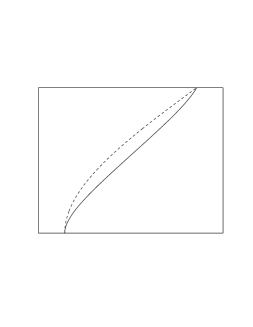
FIG. 3.: Illustration of the optimal path (8.10) for either damped propagation (solid line), or frictionless propagation (dashed line). The horizontal axis represents spatial position, while the vertical axis is for the time.

Computation of $\Delta_{R}(\tau)$ for the optimal path is straight forward. For damped propagation the computation is trivial since $\Delta_{R}\approx\eta\frac{R{-}R_{0}}{t}$ is constant. Substitution into (8.4) yields:

$${\cal K}[R_{o}]\ =\ \ const\cdot\exp\left(-\frac{1}{2}\cdot\frac{(R{-}R_{0})^{2}}{\frac{1}{\eta^{2}}\ \nu_{R}\ t}\right)\ \ \ ,$$ (8.12)

which is in consistency with the exact result of Sec.VII(A). It is easily verified that also for frictionless propagation, consistency with the exact result is maintained.

For short-time correlated colored noise ($1\leq s$) it is natural to replace $\phi(\tau{-}\tau^{\prime})$ by $\nu\delta(\tau{-}\tau^{\prime})$, with the effective white noise intensity $\nu=\phi(\omega{=}0)$. As long as $0<\nu$ (finite temperatures), the long time behavior is diffusive, and consistency with (7.5) is easily verified. Still, a more elaborated argument is required in order to substantiate the “white noise approximation”. This argument will be discussed now.

By inspection of (8.4) it is clear that the most contributing paths, for which ${\cal K}[R]$ is large, must satisfy $|\Delta_{R}(\omega)|^{2}<\phi(\omega)$. For white noise $\phi(\omega){=}\nu{=}const$, but still the “optimal path” is smooth. By “smooth” one means that $\Delta_{R}(\omega)$ is concentrated within the interval $\omega<1/\tau_{\eta}$ where $\tau_{\eta}{=}m/\eta$ is the relevant time scale for the system’s dynamics. Consider now a noise auto-correlation function of the form $\phi(\tau)=\nu\delta(\tau)+C{\cdot}G_{s}(\tau)$. Its Fourier transform satisfies $\phi(\omega)\approx\nu\approx const$ for $\omega<(\nu/C)^{1/(s{-}1)}$. Thus, the first requirement for the “white noise approximation” to hold should be $C/\tau_{\eta}^{s{-}1}<\nu$. For $\omega_{c}<\omega$ the spectral function $\phi(\omega)$ drops to zero, which implies that such high frequency components are not favored. So far there is consistency with our assumption that the most contributing paths are smooth. However, in the vicinity of $\omega_{c}$ the spectral function $\phi(\omega)$ is peaked. It implies, that unlike the case of white noise, an oscillatory component with time period $\tau_{c}$ is favored. Obviously, such component arise from the strong accelerations that the particle experiences within short periods whose duration is $\tau_{c}$. Over these short periods the maximum displacement is $\Delta L=\frac{1}{2}(\sqrt{\phi(\tau{=}0)}/m)\tau_{c}^{2}$. Using (4.6) it is found that this amplitude is proportional to $\tau_{c}^{(4{-}s)/2}$. For $s<4$ the amplitude $\Delta L$ goes to zero as $\tau_{c}\rightarrow 0$. Therefore, in this restricted regime ($1\leq s<4$), and in particular for $s=2$ (low temperature ohmic noise) the “white noise approximation” should be adequate.

B Anomalous ”Diffusion”

Encouraged by the consistency of the heuristic approach with exact results, we turn now to analyze the diffusion due to short-time correlated noise in the presence of disorder. We shall use the “white noise approximation” whose validity has been discussed in the preceding subsection. Namely, for short range correlated noise, the most contributing paths are concentrated around the same $R_{o}(\tau)$ that has been found for white noise. From (8.10) it follows that $R_{o}(\tau)$ is, up to end point transients, a free-like propagation. Consequently, the effective noise autocorrelation function is $\phi_{R}(\tau)\approx-w^{\prime\prime}((R{-}R_{0})/t\cdot\tau)\cdot\phi(\tau)$ and we define

$$\nu_{R}\ \ =\ \ \ \int_{-\infty}^{\infty}\ \ [-w^{\prime\prime}\left(\frac{R{-}R_{0}}{t}\tau\right)\cdot\phi(\tau)]\ d\tau$$ (8.13)

In general $0<\nu_{R}$, also in the limit of zero temperature.

In the presence of disorder, the effective white noise intensity is (in general) a function of the endpoint conditions, rather than a constant. For typical noise autocorrelation function of the form $\phi(\tau)=C\cdot G_{s}(\tau)$ one obtains

$$\nu_{R}\ =\ \ \tilde{C}\cdot\frac{\tau_{\ell}^{3}}{(\tau_{c}^{2}+\tau_{\ell}^{2})^{1+\frac{s}{2}}}$$ (8.14)

$$\mbox{with}\ \ \ \ \ \ \ \tau_{\ell}\ =\ \ \frac{\ell\cdot t}{(R{-}R_{0})}$$ (8.15)

$$\mbox{and}\ \ \ \ \ \ \ \tilde{C}\ =\ \ \sqrt{\frac{2}{\pi}}\ 2^{s/2}\ \Gamma(1{+}\frac{s}{2})\cdot C$$ (8.16)

The computation has been carried out by taking in (8.13) the Fourier transform of both $\phi()$ and $w^{\prime\prime}()$, and performing $d\omega$ integration rather than $d\tau$ integration. Substitution into (8.12) suggests that:

$${\cal K}(R|R_{0})\ |_{\{|R{-}R_{0}|<\ell\omega_{c}t\}}\ =\ const\cdot\exp\left(-\frac{\eta^{2}}{2\tilde{C}}\ \ell^{s{-}1}\ t^{s{-}2}\ |R{-}R_{0}|^{3{-}s}\right)$$ (8.17)

$${\cal K}(R|R_{0})\ |_{\{|R{-}R_{0}|>\ell\omega_{c}t\}}\ =\ const\cdot\exp\left(-\frac{\eta^{2}}{2\tilde{C}}\ \frac{|R{-}R_{0}|^{5}}{\omega_{c}^{s{+}2}\ \ell^{3}\ t^{4}}\right)$$ (8.18)

The “tail” of the dispersion profile is universal. It depends on $\omega_{c}$, but it is independent of the nature of the noise. In contrast, the short range profile is determined by the low frequency bath-oscillators, and thus it is sensitive to the exact value of $s$. For $s=1$, (ohmic model, high temperatures), normal diffusive behavior prevails. For $s=2$ (ohmic model, low temperatures) the diffusion freezes. The dispersion profile is Exponential rather than Gaussian, namely

$${\cal K}(R|R_{0})\ =\ \ const\cdot\exp\left(-\frac{|R-R_{0}|}{\left[4\sqrt{\frac{2}{\pi}}\ \frac{1}{\eta^{2}\ \ell}\ C\right]}\right)\ \ \ \ \ \ \ \mbox{[ohmic, low temperatures]}$$ (8.19)

The dispersion here, in the DLD model, is of the order $C/(\eta^{2}\ell)$ rather than $\sqrt{C}/\eta$. (BM model (7.6)). One should observe that on for $C\sim(\eta\ell)^{2}$ both models predict consistently dispersion on spatial scale $\ell$. For larger noise intensity, the BM model is not valid, and DLD predicts always a larger dispersion, which is intuitively expected. For weak noise ($C<(\eta\ell)^{2}$) the spatial spreading is on scale less than $\ell$. Our treatment of the DLD model is not valid on this microscopic scale. However, in this regime the BM model can be trusted. For $3<s<4$ equation (8.17) implies that the particle is evacuates from the vicinity of $R_{0}$.

The “body” of the “diffusion” profile (8.17a) is determined by a low velocity paths for which $\tau_{c}\ll\tau_{\ell}$. It is easily verified that a sufficient condition for the validity of the “white noise approximation” is $\tau_{\ell}\ll\tau_{\eta}$. This condition is satisfied in the relevant spatial range ($|R{-}R_{0}|<\ell\omega_{c}t$), except for a relatively small interval around $R_{0}$, which is determined by the large ratio $\tau_{\eta}/\tau_{c}$.

The “tail” of the “diffusion” profile (8.17b) is determined by a high velocity paths for which $\tau_{\ell}\ll\tau_{c}$. Here the the validity argument should be modified. The spectral function $\phi(\omega)$ is peaked around $\omega=1/\tau_{\ell}$ rather than around $\omega=\omega_{c}$. Thus, oscillatory component which is characterized by period $\tau_{\ell}$ is favored. The maximal spatial amplitude of this component is $\Delta L=\frac{1}{2}(\sqrt{\phi(\tau{=}0)}/m)\tau_{\ell}^{2}$. It is convenient to use a special notation for the standard deviation of the disordered potential, namely $W=\ell\sqrt{\phi(\tau{=}0)}$. Using this notation the amplitude is $\Delta L=\frac{1}{2}(W/mv^{2})\ell$. This amplitude is required to be much less than $\ell$, or alternatively $W\ll\frac{1}{2}mv^{2}$ or alternatively $\tau_{\ell}\ll\tau_{W}$, with $\tau_{W}=\ell/\sqrt{2W/m}$. In this subsection we have limited the discussion to the case of short-time correlated noise for which $\tau_{c}$ is small in some sense. Indeed, if it is assumed that $\tau_{c}\ll\tau_{W}$, then the validity condition will be satisfied automatically.

C Classical Localization and Non-Dissipative Diffusion

In this subsection we shall discuss the case of static or almost-static disordered non-dynamical environment ($\eta=0$). The “noise” is assumed to possess long-time correlations. Specifically:

$$\phi_{R}(\tau,\tau^{\prime})\ =\ -w^{\prime\prime}(R(\tau){-}R(\tau^{\prime}))\ \cdot\ \frac{W^{2}}{\ell^{2}}\exp\left(-\frac{1}{2}\frac{(\tau{-}\tau^{\prime})}{\tau_{c}}^{2}\right)\ \ \ \ ,$$ (8.20)

where $W$ is the standard deviation of the disordered potential. Here $\tau_{c}$ is assumed to be large, much larger than $\tau_{W}=\ell/\sqrt{2W/m}$.

In general the “white noise approximation” breaks down. The path integral expression is no-longer dominated by “smooth” trajectories. It is difficult to use the explicit formula (8.4) in order to identify the family of “optimal paths” since $\Phi(\tau,\tau^{\prime})$ is no longer diagonal. We therefore prefer to use heuristic considerations. No new insight is gained if one insists using (8.4).

We take first the limit $\tau_{c}\rightarrow\infty$. The classical mean free path of the particle is

$$L_{collision}\ =\ \ell\cdot\exp\left(-\frac{1}{2}\frac{\frac{1}{2}mv^{2}}{W}\right)\ \ \ \ .$$ (8.21)

The corresponding time is $T_{collision}=L_{collision}/v$. After that time the probability of being backscattered is of order 1. In one dimension this backscattering will lead to (classical) localization of the particle. The localization length is exponentially large for high energies.

If $\tau_{c}$ is finite, rather than infinite, classical localization will manifest itself only if $T_{collision}\ll\tau_{c}$. Within the time scale $\tau_{c}$, the particle spreads over spatial range of the order $L_{collision}$, while its velocity is randomized. It follows that ${\cal K}(R|R_{0})$ may be used as a stochastic kernel. Hence the Markovian property is recovered over time scales that are much larger than $\tau_{c}$, and a diffusive behavior follows with coefficient $L_{collision}^{2}/\tau_{c}$. This diffusion is non-dissipative “random walk” like.

IX Quantum Localization

As in the last subsection, we shall discuss the case of quenched disorder. However, here the quantal analysis will be carried out. The variance of the disordered potential is $W^{2}$, with auto-correlation length $\ell$. We approximate the Gaussian correlation (2.6) by a delta function. Defining $a=\sqrt{2\pi}\ell$, the path-integral expression for the propagator is (5.9) with (5.13) and

$$S_{N}[x^{\prime},x^{\prime\prime}]=\frac{1}{2}aW^{2}\int_{0}^{t}\int_{0}^{t}(\delta(x_{2}^{\prime\prime}{-}x_{1}^{\prime\prime})+\delta(x_{2}^{\prime}{-}x_{1}^{\prime})-2\delta(x_{2}^{\prime\prime}{-}x_{1}^{\prime}))d\tau_{1}d\tau_{2}$$ (9.1)

The essential feature of this functional, is its non-local nature. Our first step will be to get some insight into $S_{N}$.

Let us consider segment $i$ and segment $j$ that belong both to the same path, either $x^{\prime}$ or $x^{\prime\prime}$, within the same spatial interval $\Delta x$. This includes the possibility $i=j$. The contribution to $S_{N}$ is

$$\Delta S_{N}=+\frac{1}{2}aW^{2}\frac{\Delta x}{|v_{i}v_{j}|}$$ (9.2)

where $v$ is the velocity $\dot{x}$ within $\Delta x$. However, if $i$ belongs to $x^{\prime}$, while $j$ belongs to $x^{\prime\prime}$, or vise versa, then the contribution to $S_{N}$ is

$$\Delta S_{N}=-aW^{2}\frac{\Delta x}{|v_{i}v_{j}|}$$ (9.3)

One easily convince oneself that the contribution of each spatial interval $\Delta x$ is non-negative. A zero value may be obtained if to each segment $i$, that belongs to $x^{\prime}$, corresponds segment $j$ that belongs to $x^{\prime\prime}$, with $|v_{j}|=|v_{i}|$. For example, a zero value for $S_{N}$ may be obtained if $x^{\prime\prime}(\tau)$ is shifted in time with respect to $x^{\prime}(\tau)$. Referring to the endpoints, one should identify $\tau=t$ with $\tau=0$. It follows that $S_{N}=0$ implies that the two paths $x^{\prime}$ and $x^{\prime\prime}$ are either identical, or satisfy the constraint $R(t)=R(0)$. If $R(t)\neq R(0)$, the value $S_{N}=0$ may be obtained only if $x^{\prime}$ and $x^{\prime\prime}$ are identical. More generally, if $|v_{t}|=|v_{0}|$, one may prove that the following inequality holds for any pair of smooth paths $x^{\prime}$ and $x^{\prime\prime}$,

$$e^{-\frac{1}{\hbar^{2}}S_{N}[R,r]}\ \ \leq\ \ e^{-\frac{aW^{2}}{(\hbar v_{0})^{2}}\min(|R_{t}{-}R_{0}|,\frac{1}{2}(|r_{t}|{+}|r_{0}|))}\ \ \ .$$ (9.4)

For particular $R(\tau)$ one may ask what is the $r(\tau)$ for which $S_{N}[R,r]$ is minimal. The trivial minimum, which is also the absolute minimum, is $r(\tau)=0$, for which $S_{N}[R,r]=0$. However, any small perturbation on $r(\tau)$ will make $S_{N}[R,r]$ much larger. Therefore, we are tempted to assume that there may be some other, more stable (local) minimum $r_{R}(\tau)$. A non-trivial local minimum $r_{R}(\tau)$ does not exist for any $R(\tau)$. However, one can prove that there is a large family of $R$-s for which such minimum exists, by actually constructing them. This is done by following the considerations that were presented at the beginning of this paragraph, An example for such construction is presented in Fig.4.

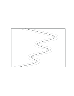
FIG. 4.: Illustration of an optimal path $R$ (solid curve) for localization problem. The dotted lines are $x^{\prime}(\tau)$ and $x^{\prime\prime}(\tau)$ that correspond to $r_{R}(\tau)$. The horizontal axis represents spatial position, while the vertical axis is for the time.

The situation here should be contrasted with that encountered in Sec.VIII. In subsection A (there) we could have defined one optimal path $R_{o}(\tau)$. Here, there is a whole family of “optimal paths”, as in the case of subsection B (there). However, in the present case these paths are “interference paths” rather than “classical paths”. The following observations concerning the relevant optimal paths are important: (a) They consist of many straight segments, and have ZigZag character; (b) The final velocity $\dot{R}(t)$ is favored to be equal in absolute value to the initial velocity; (c) Turning points impose significant restrictions; (d) The non trivial minimum $r_{R}(\tau)$ is isolated; (e) The non-trivial minimum is relatively stable. The last point is the most difficult to observe. First it should be noted that (e) must be true a-priori. Else, if the trivial minimum dominates the path-integral expression, then the result would be that the particle has roughly the same probability to go from any initial conditions to any final conditions, irrespective of proximity considerations or even energy conservation. Still, a reasonable argument is required why the non trivial minimum is relatively stable. For this consider a straight segment $i$ for which $\dot{R}(\tau)=v_{i}$ and $r_{R}(\tau)=r_{i}$. One observes that if $r_{R}$ is perturbed by a fluctuation of time period $|r_{i}|/|v|$, or by some higher harmony, then the contribution to $S_{N}[R,r]$ is negligible. This is to be contrasted with the case of the trivial minimum $r(\tau)=0$, where any fluctuation has high cost.

We turn now to the formal extension of the procedure that has been presented in the previous section. We expand $S_{N}[R,r]$ around the non-trivial minimum:

$$S_{N}[R,r]\approx S_{N}[R,r_{R}]+\int_{0}^{\infty}\int_{0}^{\infty}d\tau d\tau^{\prime}\ \phi_{R}(\tau{-}\tau^{\prime})\cdot(r(\tau){-}r_{R}(\tau))\cdot(r(\tau^{\prime}){-}r_{R}(\tau^{\prime}))\ +\ ...$$ (9.5)

Here we are not able to write an explicit expression for the highly complicated kernel $\phi_{R}(\tau{-}\tau^{\prime})$. However, we proceed, and write down the result of the Gaussian integration:

$${\cal K}[R]\ =\ \ const\cdot\cos\left(\int_{0}^{\infty}d\tau\ \Delta_{R}(\tau)r_{R}(\tau)\right)\ \mbox{e}^{-S_{N}[R,r_{R}]}\ \ \cdot$$ (9.6)

$$\cdot\ \ \exp\left(-\frac{1}{2}\int_{0}^{t}\int_{0}^{t}d\tau d\tau^{\prime}\ \Phi_{R}(\tau-\tau^{\prime})\ \Delta_{R}(\tau)\ \Delta_{R}(\tau^{\prime})\right)$$ (9.7)

Now, we should perform the ${\cal D}R$ integration. This integration will be dominated by the family of “optimal paths”. Note that the $cosine$ term in (9.6) equals unity since for $r_{R}$ the trajectories $x^{\prime}$ and $x^{\prime\prime}$ are in a sense “shifted” one with respect to the other, hence $S_{eff}=0$. Within the family of optimal paths, not all have the same contribution. One should expand around those that have the largest contribution. For these paths $S_{N}[R,r]=\frac{aW^{2}}{v_{0}^{2}}|R-R_{0}|$. Here we consider endpoints conditions $(R_{0},mv_{0})$ at $t=0$ and $(R,\pm mv_{0})$ at time $t$. The time $t$ is assumed to be sufficiently large to guaranty steady state distribution. It follows that

$${\cal K}(R,\pm mv_{0}|R_{0},mv_{0})\ \sim\ \ \exp\left(-2\frac{|R-R_{0}|}{\xi(v_{0})}\right)$$ (9.8)

where

$$\xi(v_{0})=2\cdot\frac{(\hbar v_{0})^{2}}{aW^{2}}\ \ \ .$$ (9.9)

For convenience $\hbar$ has been restored in the latter formula. In the application of the inequality (9.4) a sub-family of “optimal paths” has been ignored, for which $|r_{R}(endpoints)|<|R{-}R_{0}|$. It is justified provided this sub-family constitutes a zero fraction of the whole family. For this we should assume sufficiently long time ($t$), for which a steady state distribution is attained.

Both the validity and the applicability of the inequality (9.4) demonstrates the vulnerability of our localization argument. It is important to consider circumstances in which either of these conditions is not satisfied. The inequality (9.4) will not be valid if the noise is not infinitely correlated in time, i.e. the disordered potential is not static when viewed on large time scales. The inequality (9.4) will not be applicable if additional white noise is added to the Hamiltonian. In the latter case, large $r_{R}(\tau)$ will be suppressed by the corresponding additional term in the noise functional. Consequently, the sub-family of paths for which $|r_{R}(endpoints)|<|R{-}R_{0}|$ will not constitute zero fraction of the whole family.

Expression (9.9) for the localization length agrees with the well know result for 1D localization of “free” particle (Thouless Ref.[14]). Note that Thouless uses some scaled units, resulting in the expression $\xi=8mE/\hbar^{2}$. We shall show now that the above expression is somewhat more general, and applies also to cases where the dispersion law is different from $v=p/m$. For this one should replace in (5.11) the kinetic term $\frac{1}{2}m\dot{x}^{2}$ by some general function $T(\dot{x})$, resulting in

$$S_{free}\ =\ \int_{0}^{t}d\tau(T(\dot{x}^{\prime\prime}){-}T(\dot{x}^{\prime}))\ \approx\ \int_{0}^{t}d\tau\ p(\dot{R})\ \dot{r}\ +...$$ (9.10)

where $p(v)=T^{\prime}(v)$ is the dispersion law. The subsequent formalism is easily generalized. The expression (9.9) for $\xi$ is unaffected. Actually, the general expression for $\xi$ could have been guessed. We use naively the Born approximation, calculate the mean free path $\ell$, and rely on the fact that $\xi$ is twice the mean free path (Thouless Ref.[14]). By the golden rule, the probability of being backscattered is

$$Prob=2\pi\overline{|\langle-p|{\cal U}|p\rangle|^{2}}\cdot\frac{L}{2\pi}\frac{dp}{dE}$$ (9.11)

where $L$ is the length of the available space, and $E$ is the kinetic energy. The matrix element is

$$\overline{|\langle-p|{\cal U}|p\rangle|^{2}}=\frac{1}{L^{2}}\cdot\overline{|\mbox{FT}[{\cal U}]|^{2}}=\frac{1}{L}aW^{2}$$ (9.12)

where in the last equality FT[] denotes Fourier Transform, and ${\cal U}$ is assumed to be uncorrelated in space (“white spatial noise”). The result (9.9) is easily recovered. One should use $\xi=2\ell$, and $v_{0}=dE/dp$, while $\ell$ is evaluated via the relation $Prob=v_{0}/\ell$. In order to further demonstrate the generality of (9.9), let us consider Anderson tight binding model. The spacing will be denoted by $a$. The Hamiltonian is ${\cal H}=\sum_{n}(|n\rangle V_{n}\langle n|+T(|n\rangle\langle n{-}1|+|n\rangle\langle n{+}1|))$ where $V_{n}$ is uniformly distributed in $[-W_{0},W_{0}]$. The transition amplitude is $T$. The Kinetic energy in the center of the band is $E=2Tap$, where $p$ is the momentum. Hence $v_{0}=2Ta$ there. The dispersion of the on-site energies is $W=\frac{1}{\sqrt{12}}2W_{0}$. The “area” under the triangular autocorrelation function is $aW^{2}$. Formula (9.9) suggests that $\xi=24a(T/W_{0})^{2}$. This results agrees with that of Ref.[13] (equation (66) there), including the prefactor.

X Summary and Conclusions

A unified treatment of Diffusion Localization and Dissipation (DLD) has been presented in this work. All these phenomena may be derived from the general path integral expression (5.9),

$${\cal K}(R,P|R_{0},P_{0})=\int_{R_{0},P_{0}}^{R,P}\!\!\!{\cal D}R\int{\cal D}r\ \ \mbox{e}^{i\frac{1}{\hbar}S_{eff}[R,r]}\ \ \mbox{e}^{-\frac{1}{\hbar^{2}}S_{N}[R,r]}\ \ \ \ ,$$ (10.1)

upon inclusion of the appropriate functionals $S_{eff}$ and $S_{N}$. General expressions for these functionals are available and various limits may be considered: (a) Quantal versus classical expressions; (b) Disordered versus non-disordered environment; (c) Dissipative versus non-dissipative environment; (d) Quenched versus noisy environment. In the classical limit the DLD model constitutes a formal solution of Langevin equation. The classical limit may be obtained by linearization of the quantal $S_{eff}[R,r]$ with respect to $r$, while expanding $S_{N}[R,r]$ to be quadratic in this path-variable. The disorder or its absence depends on the choice of the spatial auto-correlation function $w(r)$. The dissipation is turned on if the friction functional $S_{F}$ is included in $S_{eff}$. The nature of the noise, whether it is “quenched”, “colored” or “white”, is determined by the noise kernel $\phi(\tau)$. In the latter case any combination may be considered as well (see further discussion at the end of this section).

The classical BM model is well defined in terms of an appropriate Langevin equation only in the case of an ohmic bath. This is not the case with the classical DLD model. The classical dynamics in the latter case is well defined in terms of appropriate Langevin equation also for non-ohmic bath. Explicit expressions for the friction force, and for the effective mass have been derived. Another nice feature of the DLD model is the absence of “switching impulse”.

Once the noise auto-correlation function $\phi(\tau)$ is specified, the BM model is in-distinguishable from its classical limit. As long as the external potential $V(x)$ is quadratic (at most), the quantal propagator is identical with the classical one, and Langevin equation can be used in order to describe correctly the time evolution of Wigner function. All the quantal effects that are associated with the standard Zwanzig-Caldeira-Leggett BM-model are (formally) reproduced by solving the classical Langevin equation with an appropriate noise term. The DLD model is different. The non-stochastic, genuine quantal features of the DLD model have been discussed. These features constitute a manifestation of either the disorder or the chaotic nature of the bath.

For either noisy or ohmic environment both the BM model and the DLD model leads to either spreading or diffusion. For the BM model, the spreading and the diffusion profiles are described by a Gaussian distribution. For the DLD model one should include a quantal correction. The disorder freezes a piece of the wavepacket, letting it to propagate as if it were a free particle. Both, the “quantal correction” to the propagator, as well as any other interference phenomena, die out exponentially in time. This exponential decay, due to dephasing, is independent of geometry. It should be contrasted with the results for loss of interference in the presence of BM-like environment [17, 18]. Another important observation is that for disordered environment, quantal interference is unaffected by friction.

On the classical level it is fascinating to analyze the diffusion profile in the presence of disorder. For the low temperature ohmic BM-model, it is found that diffusion is suppressed, though its Gaussian profile is maintained. The DLD model, in the same circumstances, leads to an exponential profile that does not change with time. This new effect is due to the interplay of the temporal (negative) autocorrelations of the noise with the spatial disorder. Even more fascinating “diffusion” profiles are found for other types of noise autocorrelations.

Quenched disorder in one dimension leads to classical localization, as well as to quantal localization. The former is characterized by a localization length which is exponentially large at high energies. Quantal localization on the other hand is dominated by interference phenomenon. We have identified the interference paths within the framework of FV formalism, and demonstrated how the well known exponential profile emerges. The localization length in the quantal case is proportional to the square of the velocity. The applicability of this result to other dispersion relations has been pointed out.

It is obvious from the derivation, that localization cannot be argued if the noise is not strictly static (e.g. slowly modulated). Diffusive behavior is recovered if the noise possess long but finite auto-correlation time. Also the case of white noise “on top” of the static disorder will evidently lead to diffusion [19][23]. In this latter case, which has not been considered in this paper, non perturbative effects may manifest themselves [20] as in the case of the “Quantum Kicked Particle” [23]. The DLD model should also account for diffusion in the presence of both quenched disorder, noisy potential and friction (all together). There should be a way to derive systematically well known heuristic results that corresponds to hopping, or variable range hopping [11].

Classical non-dissipative “random walk” diffusion has been discussed in the restricted case of long-time correlated noise. It is essential to generalize the DLD model to more than one dimension in order to account for this phenomenon in the case of strictly static disorder. Auto-correlations of the disordered potential, both in time and in space, should be considered, in order to generate the dynamics which is described by Boltzmann transport equation. In the limit of quenched disorder, localization effect should be encountered.

ACKNOWLEDGMENT

I thank Shmuel Fishman from the Technion for supporting and encouraging the present study in its initial phases. I also thank Harel Primack and Uzy Smilansky for interesting discussions and suggestions, and Yuval Gefen for his comments. The research reported here was supported in part by the Minerva Center for Nonlinear Physics of Complex systems.

A Interaction with External Bath that Consists of Extended Field Modes

This appendix illustrates how the unified formalism that has been presented in this paper should be modified in order to deal with external bath that consists of extended field modes. Unlike the case of the BM-model, this modification is not as immediate as the mere substitution of appropriate $w(r)$. In the present derivation the bath Hamiltonian is not specified, and also the assumption $u_{\alpha}=u(x{-}x_{\alpha})$ is altered.

For the standard derivation of the DLD model it has been assumed that the interaction Hamiltonian is (2.8) with $u_{\alpha}=u(x{-}x_{\alpha})$, leading to the factorized noise auto-correlation function (2.4). In the more general case the classical derivation as well as the quantal derivations lead to a stochastic force that satisfies (2.3) or to the noise functional (5.15) respectively, with noise auto-correlation function which is

$$\phi(x{-}x^{\prime},t{-}t^{\prime})=\sum_{\alpha}\phi_{\alpha}(t{-}t^{\prime})\ u_{\alpha}(x)u_{\alpha}(x^{\prime})\ \ \ .$$ (A.1)

Here $\phi_{\alpha}(t{-}t^{\prime}){=}\langle Q_{\alpha}(t)Q_{\alpha}(t^{\prime})\rangle_{eq}$  , and the interaction Hamiltonian (2.8) is used with $c_{\alpha}{=}1$ without loss of generality. The fields mode are still assumed to be decoupled, but the bath Hamiltonian is not specified. Instead, one relys on Fluctuation-Dissipation theorem as in Ref.[18], writing the general expression:

$$\phi_{\alpha}(t{-}t^{\prime})\ =\ \int_{0}^{\infty}\frac{d\omega}{\pi}J_{\alpha}(\omega)\ \hbar\coth(\frac{1}{2}\hbar\beta\omega)\ \cos[\omega(t{-}t^{\prime})]\ \ \ \ .$$ (A.2)

Note that if the field modes are simple harmonic oscillators, then one should substitute $J_{\alpha}(\omega){=}\frac{\pi}{2m_{\alpha}\omega_{\alpha}}\delta(\omega{-}\omega_{\alpha})$. Alternatively, one may speculate $J_{\alpha}(\omega)$ using known response characteristics of the bath.

To make further progress the interaction Hamiltonian (2.8) should be further specified. Using “standing waves” decomposition it is assumed to be

$${\cal H}_{int}\ =\ \sum_{\alpha}\left(Q_{1\alpha}\cos(\vec{k}_{\alpha}\cdot x)+Q_{2\alpha}\sin(\vec{k}_{\alpha}\cdot x)\right)\ \ \ \ .$$ (A.3)

Substitution of the appropriate $u_{\alpha}$ into (A.1), and converting the summation to an integral over directions and over $k$, the result can be cast into the following form

$$\phi(x{-}x^{\prime},t{-}t^{\prime})\ =\ \int_{0}^{\infty}\frac{k^{d{-}1}dk}{\pi}\phi(k,t{-}t^{\prime})\ \langle\cos(k\hat{\Omega}\cdot(x{-}x^{\prime}))\rangle_{\Omega}\ \ \ \ .$$ (A.4)

The average over directions can be performed leading to $\cos(k|x{-}x^{\prime}|)$ in 1-D, Bessel function ${\cal J}_{0}(k|x{-}x^{\prime}|)$ in 2-D, and $\mbox{sinc}(k|x{-}x^{\prime}|)$ in 3-D.

In Ref.[18] the interaction with electromagnetic fluctuations in metal has been considered. It has been assumed that each mode is characterized by an ohmic response. In our notations it corresponds to $J(k,\omega)=\eta(k){\cdot}\omega$. Due to this assumption, the noise auto-correlation function becomes factorized at high temperatures, as in the DLD model. In particular, for the noise functional (5.15) one obtains

$$S_{N}[r]\ =\ \int_{0}^{t}d\tau\ \frac{1}{\beta}\int_{0}^{\infty}\frac{k^{d{-}1}dk}{\pi}\ \eta(k)\ \langle\sin^{2}(k\hat{\Omega}\cdot r(\tau))\rangle_{\Omega}\ \ \ \ .$$ (A.5)

For the discussion of dephasing, we write again this result using the notations of Ref.[18]. It is assumed that $\eta(k)=e^{2}/(\sigma k^{2})$, where $e$ is the charge of the electron and $\sigma$ is the conductivity. Integration over $k$ leads to the result

$$\langle\mbox{e}^{i\varphi}\rangle\ =\ \ \exp\left[-\frac{e^{2}k_{B}T}{2\hbar^{2}\sigma}\int_{0}^{t}\ |x_{a}(\tau)-x_{b}(\tau)|^{2-d}\ d\tau\right]\ \ \ \ \mbox{for $d\leq 2$}\ .$$ (A.6)

This result, that has been obtained in Ref.[18] (equation (7.8) there), is very similar to the corresponding result (6.17) for the BM-model, the difference being the power $(2{-}d)$ which is not universal.

An apparently simpler example for an interaction with external bath that consists of extended field modes, is the electron-phonon interaction. Here we want to question the applicability of the BM model as an approximated description. The electron is assumed to be confined to a one dimensional “quantum wire”, while the phonons dwell in the 3-D bulk. Considering longitudinal modes, the coupling of the $\alpha\rightarrow(k_{1},k_{2},k_{3})$ “oscillator” with the electron is $k_{1}\cdot x$, with a coupling constant $C_{\alpha}\propto\sqrt{k_{1}^{2}+k_{2}^{2}+k_{3}^{2}}$. Summing over $\alpha$, as defined in (2.11), one obtains effectively $J(\omega)\propto\omega^{d+2}$ where $d{=}3$ is the dimensionality of the space where the phonons dwell. Thus a phonons-bath is similar to a superohmic BM-model. However, this derivation is somewhat miss-leading, since a cutoff $\omega_{c}$ should be introduced, while for the original electron-phonon interaction a natural cutoff $|x{-}x^{\prime}|/c$ exists.

B An Interference Gedanken Experiment

In this appendix we consider the interference phenomenon from two different points of view, and demonstrate their consistency. First we consider the free propagation of two-wavepackets superposition. The decay of the interference pattern will be dictated by the propagator (7.12). Then we consider the scattering of a simple wavepacket from a double-barrier. The suppression of interference paths will be dictated by the noise functional (Sec.VI(C)). Finally, we argue that both points of view are physically equivalent, and must lead to the same result, which is indeed the case.

Consider a superposition of two Gaussian wavepackets which have the same momentum $P_{0}$, the same initial spatial spreading $\sigma_{0}$, while their initial locations satisfies $|R_{02}{-}R_{01}|{=}d$. The Wigner function for this preparation is easily computed, and is of the form

$$\rho_{t{=}0}(R,P)\ =\ \frac{1}{2}G(R{-}R_{01},P{-}P_{0})\ +\ \frac{1}{2}G(R{-}R_{01},P{-}P_{0})\ +\ \cos\left(\frac{P-P_{0}}{\delta P_{c}}\right)\cdot G(R{-}\frac{1}{2}(R_{01}{+}R_{02}),P{-}P_{0})\ \ \ \ ,$$ (B.1)

where $G(x,p)$ denotes “minimum-uncertainty” Gaussian distribution, and $\delta P_{c}{=}\hbar/d$. For free propagation $\rho_{t}(R,P)$ will develop fringes on the spatial scale $\Delta x{=}\frac{\delta P_{c}}{m}{\cdot}t\$. Note that this gedanken experiment is formally equivalent to the usual “two slit” diffraction experiment upon the definition $\Delta\theta=\frac{\Delta x}{v{\cdot}t}=\frac{\hbar}{P_{0}}/d$. For propagation in noisy non-disordered environment the interference pattern is smeared on scale $\delta P\sim\nu{\cdot}t$, due to the diffusive momentum spreading. The smearing factor is $\exp[-\frac{1}{2}(\delta P(t)/\delta P_{c})^{2}]$ leading to an exponential decay $\exp[-\frac{\nu d^{2}}{\hbar^{2}}t]$, that depends on the separation $d$. On the other hand, for propagation in noisy disordered environment, using (7.12), the exponential decay is $\exp[-\frac{\nu\ell^{2}}{\hbar^{2}}t]$, independent of geometry.

Consider now scattering problem in one dimension. The potential is assumed to be $V(x){=}\infty$ for $x<0$, and $V(x)=\delta(x{-}\frac{d}{2})$ for $0<x$. A simple Gaussian wavepacket with momentum $-P_{0}$ and spatial spreading $\sigma_{0}\ll d$ is launched from $R_{0}$. The scattered particle is detected at the range $R$ which is assumed to be much larger than $R_{0}$. In the absence of noise and dissipation, it is not difficult to work out the explicit solution of this scattering problem. A “train” of Gaussian-like wavepackets will emerge from the scattering region. The spatial separation between each two wavepackets is $d$, and the probability density function will contain interference pattern in between. From the FV path-integral point of view (Sec.VI(C)), the interference pattern is due to the existence of “interference paths”. In the presence of noisy disordered environment the contribution of these interference paths to the propagator is suppressed exponentially in time.

Assuming that the dephasing during the time interval $t_{scattering}{=}R_{0}/v$ is negligible, one may use the results of the first gedanken experiment, leading to the same exponential decay. Thus, the result (7.12) for the propagator is consistent with the analysis of interference in Sec.VI(C). Our gedanken experiment can be used also in order to illustrate and clarify the observation that friction does not affect the interference phenomenon. This observation holds for disordered dynamical environment.

REFERENCES

- [1] H.A. Kramers, Physica 7, 284 (1940).
- [2] W.H. Louisell, Quantum Statistical Properties of Radiation, (Wiley, London, 1973).
-
[3]
R. Zwanzig, J. Stat. Phys. 9, 215 (1973).
D.H.E. Gross, Nuclear Physics A240, 472 (1975); Z. Physik A 291, 145 (1979). -
[4]
H. Grabert, P. Schramm and G.L. Ingold,
Phys. Rep. 168, 115 (1988).
P. Hänggi, P. Talkner and M. Borkovec, Rev. Mod. Phys. 62, 251 (1990). - [5] R.P. Feynman and F.L. Vernon Jr., Ann. Phys. (N.Y.) 24, 118 (1963).
- [6] K. Möhring and U. Smilansky, Nuclear Physics A338, 227 (1980).
-
[7]
A.O. Caldeira and A.J. Leggett, Ann. Phys. (N.Y.)
140, 374 (1983);
Physica 121 A, 587 (1983). - [8] V. Hakim and V. Ambegaokar, Phys. Rev. A 32, 423 (1985).
-
[9]
Y. Gefen and D.J. Thouless, Phys. Rev. Lett.
59, 1752 (1987).
E. Shimshoni and Y. Gefen, Annals of Physics 210, 16 (1991). - [10] M. Wilkinson, J. Phys. A: Math. Gen. 21, 4021 (1988).
-
[11]
N.F. Mott and E.A. Davis, Electronic Processes in
Non-Crystalline Materials,
(Clarendon Press, Oxford, 1971). -
[12]
I.M. Lifshits, S.A. Gredekul and L.A. Pastur,
Introduction to the Theory of Disordered Systems,
(John Wiley and Sons, 1988). - [13] B. Kramer and A. MacKinnon, Rep. Prog. Phys., 56, 1469 (1993).
- [14] D.J. Thouless, J. Phys. C 5, 77 (1972); J. Phys. C 6, L49 (1973).
- [15] A.M. Jayannavar and N. Kumar, Phys. Rev. Lett. 48, 553 (1982).
- [16] S. Marianer and J.M. Deutsch, Phys. Rev. B 31, 7478 (1985).
- [17] B.L. Al’tshuler, A.G. Aronov and D.E. Khmelnitskii, J. Phys. C 15, 7367 (1982).
- [18] A. Stern, Y. Aharonov and Y. Imry, Phys. Rev. A 41, 3436 (1990).
- [19] E. Ott, T.M. Antonsen Jr. and J.D. Hanson, Phys. Rev. Lett. 53, 2187 (1984).
- [20] F. Borgonovi and D.L. Shepelyansky, Adiabatic Destruction of Anderson Localization (preprint, 1994).
- [21] D. Cohen and S. Fishman, Phys. Rev. A 39, 6478 (1989).
- [22] D. Cohen, J. Phys. A 27, 4805 (1994).
- [23] D. Cohen, Phys. Rev. Lett. 67, 1945 (1991); Phys. Rev. A 44, 2292 (1991).
- [24] M.V. Berry and J.M. Robbins, Proc. R. Soc. London A 442, 659 (1993).
- [25] J. Sanchez Canizares and F. Sols, Physica A 212, 181 (1994).
- [26] A different type of generalized BM model, using (2.8) with e.g. quadratic has been introduced by Lindenberg et al. (Physica A 126, 489 (1984)). The latter type of generalization has been used by Straus et. al. (J. Chem. Phys. 98, 4082 (1993)) in order to study position dependent friction.