Penumbra diffraction in the quantization of concave billiards

Abstract

The semiclassical description of billiard spectra is extended to include the diffractive contributions from orbits which are nearly tangent to a concave part of the boundary. The leading correction for an unstable isolated orbit is of the same order as the standard Gutzwiller expression itself. The importance of the diffraction corrections is further emphasized by an estimate which shows that for any large fixed $k$ almost all contributing periodic orbits are affected. The theory is tested numerically using the annulus and the Sinai billiard. For the Sinai billiard the investigation of the spectral density is complemented by an analysis which is based on the scattering approach to quantization. The merits of this approach as a tool to investigate refined semiclassical theories are discussed and demonstrated.

• †Department of Physics of Complex Systems, The Weizmann Institute of Science, Rehovot 76 100, Israel

• ‡Institut für Physik, Humboldt-Universität, 10 099 Berlin, Germany

1 Introduction

Beside the generic orbits which chaotic billiards support, there may exist important families of non-generic orbits, which affect the dynamics, and play a prominent rôle when the billiards are quantized semiclassically. The bouncing ball orbits which reflect between straight sections of the boundaries are an important example which was studied extensively in the past [1, 2] and will not be dealt with here. Another type exists in convex billiards (or along convex sections), and it comprises of whispering gallery orbits: these are classical trajectories which provide a hierarchy of polygonal approximants to the boundary. A detailed study of the rôle of such orbits in the quantization of convex and smooth boundaries is given in [3]. The particular case of the stadium billiard, to which Lazutkin’s theory does not apply, was studied in [2, 4]. The whispering gallery orbits occupy a narrow strip in phase space, limited on one side by the boundary of the phase space domain. In the case of a smooth, convex billiard, every point on the phase space boundary is a fixed point of the bounce map. We can therefore consider the boundary as a one-parameter family of fixed points, which is the limit of the family of whispering gallery orbits.

Figure 1: The quarter Sinai billiard and the attached waveguide.

In the present paper, we shall focus our attention on concave billiards, where the whispering gallery modes do not appear. Instead, concave billiards are characterized by the existence of tangent orbits along the concave sections of the boundary. They also form a one parameter family, which belongs to the boundary of the phase space domain. In this sense they are the counterparts of the whispering gallery orbits in convex billiards. In contrast to convex billiards, however, tangency introduces discontinuities in the classical map, and therefore the set (of zero measure) of tangent orbits is excluded from the classical phase space when the ergodic properties of the billiards are studied. Tangency is also responsible for a special kind of bifurcation which can be best illustrated by considering the standard Sinai billiard, or rather, its desymmetrized quarter (see figure 1). This will be the example we shall use throughout this article and it can be generalized to other chaotic concave billiards in a straightforward manner. The chord $AB$ in figure 1 is tangent to the arc of radius $R_{0}$ and it is a classical trajectory which leads from $A$ to $B$. Bifurcations due to tangency occur when one allows the radius of the arc to vary. When the radius is reduced to any value $R_{-}<R_{0}$, two classical trajectories can serve to connect $A$ and $B$. One of them goes directly, the other reflects specularly from the arc at a point $C$. As $R_{-}\rightarrow R_{0}$ the two trajectories become closer, until they coalesce when $R_{-}=R_{0}$. When the radius is increased to values $R_{+}>R_{0}$, both the direct and the reflected trajectories from $A$ to $B$ become classically forbidden. That is, $A$ and $B$ are mutually shaded from each other by the geometrical shadow cast by the arc.

Tangency affects also the quantum (wave) dynamics in the billiard. Due to the finite wave length, the sharp geometrical shadow is replaced by a transition region which smoothly interpolates between the strictly illuminated and shaded regions. This is the penumbra (Latin: almost shadow) domain. The standard semiclassical quantization of billiards, which is restricted to the illuminated domain, expresses the density of states $d(k)\equiv\sum_{n}\delta(k-k_{n})$ ($E_{n}=k_{n}^{2}$ are the eigenvalues) in terms of classical periodic orbits via the Gutzwiller trace formula [5]. A semiclassical theory for transitions to the strictly shaded domain can be formulated in terms of non-classical orbits which are allowed to creep along a section of the boundary. This approach was first discussed by Keller and co-workers who developed the concept of geometrical diffraction theory in a systematic way [6]. Vattay et al. [7] have recently generalized Gutzwiller’s trace formula by including periodic orbits with creeping sections that give exponentially small corrections. In a previous paper [8] we gave a preliminary account of a semiclassical theory which is valid in the penumbra where the diffraction contributions are not exponentially small. The purpose of the present paper is twofold - to give a complete discussion of the penumbra effects, and to show how they can be scrutinized within the scattering approach to quantization [9, 10, 11, 12].

Diffraction effects appear as corrections to the leading semiclassical expressions which are based on Gutzwiller’s trace formula. To identify corrections to the contributions from individual periodic orbits, it is advantageous to study the “length spectrum”

$$D(x)=\int_{0}^{\infty}{\rm d}k\,{\mathrm{e}}^{{\mathrm{i}}kx}d(k)=\sum_{n=1}^{\infty}e^{{\mathrm{i}}k_{n}x}\,.$$ (1)

Strictly speaking, $D(x)$ is a tempered distribution whose singular support is at lengths of periodic manifolds of the classical billiard [13]. In the Sinai billiard these are the continuous families of neutral orbits (bouncing ball manifolds) and isolated unstable periodic orbits. In practice, we do not have the complete spectrum at our disposal, and we study the truncated length spectrum

$$D_{w}(x)=\int_{0}^{\infty}{\rm d}k\,{\mathrm{e}}^{{\mathrm{i}}kx}w(k)d(k)\,=\sum_{n=1}^{\infty}w(k_{n})\,{\mathrm{e}}^{{\mathrm{i}}k_{n}x}\,.$$ (2)

Here $w(k)$ is a smooth positive function with a finite support centered at $k=\bar{k}$. $D_{w}(x)$ is a smooth function with finite spikes where $D(x)$ is singular. The leading semiclassical contributions to (2) can be evaluated by substituting the Gutzwiller trace formula, augmented with the special expressions due to the neutral families. The difference between the semiclassical and the exact length spectra gives a measure of the quality of the semiclassical approximation. We shall show below that the corrections due to diffraction effects are responsible for the largest deviations. The main difficulty of this approach is that the length spectrum for a chaotic billiard is rather dense, and even with spectral sections containing thousands of eigenvalues, the contributions from neighbouring lengths overlap to the extent that a detailed investigation of contributions from individual periodic orbits is impossible. However, the scattering approach to quantization offers a method to disentangle some of this complexity which is due to the proliferation of periodic orbits.

The scattering approach we shall employ here makes use of an auxiliary scattering system which couples the billiard to a wave guide in an appropriate manner [9, 10, 11, 12]. In a way, this method provides the quantum analogue of the classical Poincaré section in terms of the scattering matrix, and it has much in common with earlier [14] and later [15, 16] attempts aiming at a similar goal. Since the method is well documented and reviewed, we shall only mention its basic ingredients for the particular application to the Sinai billiard.

The scattering problem which we use in the present context is described in figure 1. We define two systems to which we apply the Krein spectral shift theorem [17]. The Hamiltonian $H_{0}$ of the first system is the kinetic energy ($-\Delta$) in the space of functions which satisfy Dirichlet boundary conditions on the parallel channel walls and on the section $\Gamma_{\rm S}$ which separates the original Sinai billiard from the wave guide. In the second system $H$ the wall at $\Gamma_{\rm S}$ is not present and the functions under consideration have to satisfy Dirichlet boundary conditions on the extended billiard boundary displayed with a full line in figure (1). One can now define the scattering matrix $S(E)$ for any energy $E=k^{2}$, and at the energy eigenvalues $E_{n}$ of the billiard the secular equation $\det(I+S(E_{n}))=0$ is satisfied. Krein’s theorem is expressed by the relation

$$\frac{1}{\pi}\lim_{\epsilon\downarrow 0}{\rm Im}\,{\rm Tr}\,\left[G(E+i\epsilon)-G_{0}(E+i\epsilon)\right]=\frac{1}{2\pi}\frac{{\mathrm{d}}\Theta(E)}{{\mathrm{d}}E}\,.$$ (3)

The trace in (3) is taken over the space of continuum eigenstates of $H$. $G_{0}$ and $G$ are the Green functions for the two systems ($G_{0}$ is zero inside the billiard domain), and $\Theta(E)$ is the total phase of the scattering matrix $S(E)$, defined by $\Theta(E)=-{\mathrm{i}}\,\log\det S(E)$. Krein’s theorem connects the excess density of continuum states due to the introduction of the scatterer, with the total phase of the S-matrix. Performing the trace operation in the semiclassical approximation (see e.g. [18, 19]), one finds that the left hand side in (3) can be expressed as a sum of a smooth term and contributions from trapped periodic orbits - orbits which do not escape in spite of the fact that the billiard is opened. This is very important in the context of the semiclassical quantization of billiards by the scattering approach. There, one expresses the spectral density of the closed billiard as

$$d(k)=\frac{1}{2\pi}\frac{{\mathrm{d}}\Theta(k)}{{\mathrm{d}}k}+\frac{1}{\pi}{\rm Im}\,{{\mathrm{d}}\over{\mathrm{d}}k}\sum_{n=1}^{\infty}\frac{(-1)^{n}}{n}\mathop{\mathrm{T}r}\nolimits\,S^{n}(k)\,.$$ (4)

In the semiclassical limit, each ${\rm Tr}\,S^{n}$ is expressed as a sum of contributions from the periodic orbits of the closed billiard which bounce on the section $\Gamma_{\rm S}$ exactly $n$ times. However, there may be periodic orbits which do not reflect from $\Gamma_{\rm S}$ at all. They are trapped in the open billiard, and their contributions to the level density come from the semiclassical expression of $\frac{1}{2\pi}\frac{{\mathrm{d}}\Theta(k)}{{\mathrm{d}}k}$ via (3), as explained above [9]. $\frac{1}{2\pi}\frac{{\mathrm{d}}\Theta(k)}{{\mathrm{d}}k}$ provides also the leading term in the expression for the smooth part of the spectral density. It contains higher order contributions as well, but not necessarily all of them, as is discussed in [20].

Taking the Fourier transform of (4), we get an expression of the length spectrum in terms of the Fourier transforms of $\frac{1}{2\pi}\frac{{\mathrm{d}}\Theta(k)}{{\mathrm{d}}k}$ and of $\frac{{\mathrm{d}}{\rm Tr}\,S^{n}(k)}{{\mathrm{d}}k}$ for all positive $n$. The transform of the total phase will provide the length spectrum of orbits which are trapped in the open billiard. In our system there exists only one isolated and unstable trapped orbit. Another contribution comes from the family of marginally stable orbits which bounce perpendicularly between the straight sections of the billiard. This is a very sparse set of lengths, and it leaves a lot of space to observe diffractive orbits of various kinds. The Fourier transform of $\frac{{\mathrm{d}}{\rm Tr}\,S^{n}(k)}{{\mathrm{d}}k}$ provides the length spectrum of orbits which bounce $n$ times from the section $\Gamma_{\rm S}$. In this way we can partition in a systematic way the contribution from orbits with different $n$ to the total length spectrum and next to leading order effects such as diffraction contributions can be better observed.

To have an idea of the way how the theory which was described above works in practice, let us consider the simple case of the square billiard. Denoting the length of the square by $a$, we get a diagonal scattering matrix

$$S_{l,l^{\prime}}(k)=-\exp\left[2\pi{\mathrm{i}}\sqrt{\left(\frac{ak}{\pi}\right)^{2}-l^{2}}\,\right]\delta_{ll^{\prime}}\,.$$ (5)

The subspace of conducting modes is of dimension $\Lambda=\left[\frac{ak}{\pi}\right]$, where the symbol $\left[\cdot\right]$ stands here for the integer part. In this case

$$\frac{1}{2\pi}\Theta(k)=\sum_{l=1}^{\Lambda}\sqrt{\left(\frac{ak}{\pi}\right)^{2}-l^{2}}-\frac{\Lambda}{2}$$ (6)

Using the Poisson summation formula and other standard relations, one gets

$$\frac{1}{2\pi}\Theta(k)=\frac{a^{2}k^{2}}{4\pi}-\frac{ak}{\pi}+\frac{1}{4}+\frac{ak}{2\pi}\sum_{m=1}^{\infty}\frac{1}{m}J_{1}(2mak)-\frac{1}{2\pi}\sum_{m=1}^{\infty}\frac{1}{m}\sin(2mak)\,.$$ (7)

This is an exact equality which can be interpreted in the following way. The expression appearing in the upper line of (7) is the smooth spectral counting function $\bar{N}(k)$ which consists of three terms only - the area, circumference and corners terms [21]. The next infinite sum is the contribution of the (open) manifold of periodic orbits which are parallel to the section $\Gamma_{\rm S}$. The last sum is due to to the limiting periodic orbits which run along the edge $\Gamma_{\rm S}$ and its counterpart on the other side of the billiard. These two limiting orbits are the closure of the manifold mentioned previously. We thus see that the oscillatory part of (7) consists of contributions which exhaust all possible trapped periodic motion in the open billiard. We would like to emphasize again that this result is exact. In the sequel, when we treat the more interesting Sinai billiard, we shall obtain similar relationships which involve other possible trapped orbits. This will be done, however, within the semiclassical approximation and its refinements.

The paper is organized in the following way. In the next section we shall present the semiclassical theory of quantization for billiards which are exterior to a circle taking into account the leading diffraction effects both in the penumbra and the deep shadow domains. Once this is achieved, we demonstrate the success of the theory using two numerical examples. The first example in section 3 will be the annular sector which represents an integrable billiard. In the following section 4 we turn to a detailed numerical study of the quantized Sinai billiard which is chaotic and therefore necessitates the methods of analysis which were outlined above. In section 5 we shall discuss the general significance of diffraction corrections for the semiclassical quantization of a concave and chaotic billiard. The results of the paper will then be summarized in section 6.

2 Theory of diffraction for dispersing billiards

In this section, we consider billiards with a domain $\Omega$ that is exterior to a circle (e.g. the Sinai billiard). We find expressions for the contribution to the density of states of periodic orbits which are nearly tangent to the circle (either by reflecting with a very small angle or by passing very close to the circle). As will be shown, the standard semiclassical expressions for contributions of such orbits fail. In addition creeping orbits [6] exist due to the concave billiard boundary (the circle in our case). The contribution of periodic orbits which have a creeping part was studied by Vattay, Wirzba and Rosenqvist [7]. However, their expressions for creeping orbits also fail, if the orbit is too close to tangency (i.e. if the creeping angle is too small). The expressions for periodic orbits near tangency, derived in this section, extend the semiclassical description of a general billiard exterior to a circle. The methods we will use for nearly tangent periodic orbits are adapted from the calculations of Nussenzveig [22] for the problem of scattering off a three-dimensional sphere.

The free Green function satisfies

$$(\Delta+k^{2})\,G({\bf r},{\bf r}^{\prime})=-\delta({\bf r}-{\bf r}^{\prime})$$ (8)

for any ${\bf r},{\bf r^{\prime}}$ and outgoing boundary conditions at infinity. From Green’s theorem one obtains that the eigenvalues $k_{n}$ of the billiard are those values for which the boundary integral equation

$$u({\bf r}_{s})=2\int_{\Gamma}{\rm d}s^{\prime}\,\frac{\partial G}{\partial\hat{n}_{s}}({\bf r}_{s},{\bf r}_{s^{\prime}})u({\bf r}_{s^{\prime}})$$ (9)

for the normal derivative of the wave function $u({\bf r}_{s})=\partial\psi/\partial\hat{n}({\bf r_{s}})$ has a solution. The billiard boundary is denoted by $\Gamma$, and the normal direction $\hat{n}_{s}$ in a point on the boundary ${\bf r_{s}}$ is pointing from $\Omega$ outwards.

Equation (9) is used to obtain a secular equation, from which the density of states $d(k)$ may be found by a multiple reflection expansion containing terms as

$${\rm Im}\frac{2^{N}}{\pi N}\frac{{\mathrm{d}}}{{\mathrm{d}}k}\int_{\Gamma}{\rm d}s_{1}\ldots{\rm d}s_{N}\frac{\partial G}{\partial\hat{n}_{1}}({\bf r}_{1},{\bf r}_{2})\cdots\frac{\partial G}{\partial\hat{n}_{N-1}}({\bf r}_{N-1},{\bf r}_{N})\frac{\partial G}{\partial\hat{n}_{N}}({\bf r}_{N},{\bf r}_{1})\,.$$ (10)

When the integrals are evaluated in stationary phase approximation, each saddle point in one of these terms yields the contribution of a periodic orbit which reflects $N$ times off the boundary. This method has often been used as a starting point to derive semiclassical theories for billiards, e.g. Alonso and Gaspard employed it for finding higher order corrections to the contributions of periodic orbits [23].

For the purpose of considering nearly tangent or creeping orbits at the circle, the free Green function is replaced by the circle Green function, which will also be denoted by $G$. It satisfies (8) for ${\bf r}$ and $\bf r^{\prime}$ exterior to the circle, and moreover the prescribed boundary conditions on the circle. The derivation of (10) may still be followed and yields the contribution of periodic orbits which reflect $N$ times off $\Gamma$, which is now the billiard boundary excluding the circle. The reflections off the circle are included in the Green function, and so is the diffractive behaviour associated with creeping or nearly tangent orbits. The problem is thus reduced to understanding the behaviour of the Green function of the circle for different positions of $\bf r$ and $\bf r^{\prime}$.

Although in principle the multiple reflection expansions based on the free and the circle Green functions are equivalent and both exact, the latter greatly simplifies the mathematical treatment close to tangencies. A hint to this is already contained in the classical analogue representing a Poincaré map from the boundary $\Gamma$ to itself, which is discontinuous when the circle is a part of $\Gamma$. The same system can be described by a mapping which is $C^{(0)}$ when the circle is excluded from $\Gamma$ and the mapping function includes the reflection the circle.

2.1 The circle Green function

In this section we consider a circle of radius $R$ centered at the origin, with Dirichlet boundary conditions ($\psi({\bf r})=0$) on its boundary. In Appendix A we indicate how the results of this section modify for Neumann ($\partial_{\bf\hat{n}}\psi({\bf r})=0$) or mixed boundary conditions ($\kappa\psi({\bf r})+\partial_{\bf\hat{n}}\psi({\bf r})=0)$.

The Green function of the circle satisfies (8) for any $\bf r$, $\bf r^{\prime}$ outside the circle, outgoing boundary conditions at infinity, and Dirichlet boundary conditions on the circle. The exact expression for the Green function is (in polar coordinates)

$$G({\bf r},{\bf r^{\prime}})=\frac{{\mathrm{i}}}{8}\sum_{l=-\infty}^{\infty}\left[H_{l}^{-}(kr_{<})+S_{l}(kR)H_{l}^{+}(kr_{<})\right]H_{l}^{+}(kr_{>}){\mathrm{e}}^{{\mathrm{i}}l\Delta\theta}\,,$$ (11)

where $r_{>}$ ($r_{<}$) is the larger (smaller) of $r$ and $r^{\prime}$, and $\Delta\theta=\theta-\theta^{\prime}$. The elements of the scattering matrix of the circle which is diagonal in the angular momentum representation are given by

$$S_{l}(kR)=-\frac{H_{l}^{-}(kR)}{H_{l}^{+}(kR)}\,.$$ (12)

We continue the discussion assuming $r,r^{\prime}\mathchar 13606\relax[1+(kR)^{-2/3}]R$, so that the Debye approximation may be used for $H_{l}^{+}(kr)$ and $H_{l}^{+}(kr^{\prime})$ if $l\leq kR$. In addition we assume, without loss of generality, that $0<\Delta\theta<\pi$.

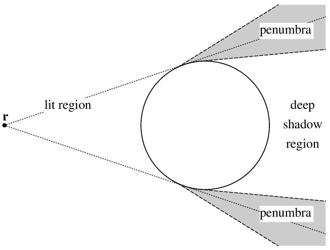
Figure 2: The different regions of $\bf r^{\prime}$ for a given $\bf r$. The penumbra occupies a small region on both sides of the geometrical shadow line (dotted).

The Poisson summation rule is used to express the Green function as

$$G({\bf r},{\bf r^{\prime}})=\sum_{m=-\infty}^{\infty}G^{(m)}({\bf r},{\bf r^{\prime}})\,,$$ (13)

where

$$G^{(m)}({\bf r},{\bf r^{\prime}})=\frac{{\mathrm{i}}}{8}\int_{-\infty}^{+\infty}{\rm d}l\,\left[H_{l}^{-}(kr_{<})+S_{l}(kR)H_{l}^{+}(kr_{<})\right]H_{l}^{+}(kr_{>}){\mathrm{e}}^{{\mathrm{i}}l\Delta\theta+2\pi iml}\,.$$ (14)

We discuss separately three regions for r and r’ (see figure 2). The first is the lit region, in which the usual semiclassical results hold. It is obtained from the $m=0$ term in (13), while the $m\neq 0$ terms always describe the contributions of creeping waves. The second is the deep shadow region, in which only creeping waves contribute and the third is the penumbra, in which the leading order contribution, the $m=0$ term, comes from nearly tangent orbits. The lit and the deep shadow regions lead to known contributions of periodic orbits and the corresponding derivations will only briefly be described for the sake of completeness, and for understanding where the employed approximations fail when approaching the transition region.

2.1.1 The lit region

Figure 3: The geometry of trajectories in the lit region (in the upper part) and of creeping trajectories in the deep shadow region (in the lower part).

In the lit region the integral $G^{(0)}({\bf r},{\bf r^{\prime}})$ gives the usual semiclassical result. For the scattering matrix element $S_{l}(kR)$ the Debye approximation is used for $l<kR$, and for $l>kR$ it is approximated by $1$. The integral is evaluated in stationary phase approximation. There are two saddle points, which relate to the two classical trajectories from $\bf r$ to $\bf r^{\prime}$ (see figure 3). One is direct, and the other reflects specularly from the circle. The Green function is then a sum of two terms. The contribution of the direct path is given by

$$G_{\rm d}({\bf r},{\bf r^{\prime}})=\frac{1}{4}\left(\frac{2{\mathrm{i}}}{\pi kL}\right)^{\frac{1}{2}}{\mathrm{e}}^{{\mathrm{i}}kL}\,,$$ (15)

where $L=|{\bf r}-{\bf r^{\prime}}|$, and the reflected path yields

$$G_{\rm r}({\bf r},{\bf r^{\prime}})=-\frac{1}{4}\left[\frac{2{\mathrm{i}}}{\pi k(L_{\rm r}+L_{\rm r^{\prime}}+2L_{\rm r}L_{\rm r^{\prime}}/a)}\right]^{\frac{1}{2}}{\mathrm{e}}^{{\mathrm{i}}k(L_{\rm r}+L_{\rm r^{\prime}})}\,,$$ (16)

where $L_{\rm r}$ ($L_{\rm r^{\prime}}$) is the distance from $\bf r$ ($\bf r^{\prime}$) to the point of reflection such that the length of the reflected trajectory is $L_{\rm r}+L_{\rm r^{\prime}}$. The impact parameter of the reflected path is $b_{\rm r}$, and $a=\sqrt{R^{2}-b_{\rm r}^{2}}$.

The semiclassical result fails when the reflected trajectory becomes nearly tangent to the circle. To be precise, the semiclassical approximation holds provided that $b_{\rm r}\mathchar 13614\relax[1-(kR)^{-2/3}]R$. In other words the angle of incidence $\theta$ should be smaller than $\pi/2-(kR)^{-1/3}$. This condition is necessary for the semiclassical approximation of the scattering matrix $S_{l}(kR)$ to hold at the saddle point, and thus defines the borderline between the illuminated region and the penumbra.

2.1.2 The deep shadow region

Figure 4: The complex $l$ plane. The squares represent the poles of the $S$ matrix. The bold line shows the contour from $\sigma_{1}\infty$, going through $kR$ and around the poles of the $S$ matrix to $\sigma_{2}\infty$. The contour does not cross the two lines defined by (21)-(22), with $\eta\rightarrow\pm\pi/2$.

In the deep shadow region the contour of the integral (14) for $m=0$ may be closed in the upper half plane. The integral is then calculated by summing the contributions of the poles of the integrand which are just the poles of the $S$ matrix. The first few poles are close to $kR$ (figure 4) and give a contribution which is evaluated using the transition region approximation for the Hankel functions. The position of these poles is given by

$$l_{n}\approx kR+{\mathrm{e}}^{{\mathrm{i}}\pi/3}x_{n}\left(\frac{kR}{2}\right)^{\frac{1}{3}}\,,$$ (17)

where $-x_{n}$ are the zeros of the Airy function ${\rm Ai}(x)$ [24]. The residues of the $S$ matrix at these poles are given by

$$r_{n}\approx\frac{{\mathrm{e}}^{-i\pi/6}}{2\pi{\rm Ai}^{\prime}(-x_{n})^{2}}\left(\frac{kR}{2}\right)^{\frac{1}{3}}\,.$$ (18)

The result is interpreted as the contribution of a creeping wave [6]. It starts from $\bf r$ along a path which is tangent to the circle and creeps along the circle in one of the available creeping modes $n$ until it leaves to $\bf r^{\prime}$ along a path which is again tangent to the circle (see figure 3). The contribution of a creeping wave to the Green function is

$$G_{\rm c}^{(0)}({\bf r},{\bf r^{\prime}})=\frac{1}{4}\left(\frac{2{\mathrm{i}}}{\pi kL_{\rm r}L_{\rm r^{\prime}}}\right)^{\frac{1}{2}}{\mathrm{e}}^{{\mathrm{i}}k(L_{\rm r}+L_{\rm r^{\prime}})}\sum_{n}D_{n}^{2}{\mathrm{e}}^{{\mathrm{i}}l_{n}\gamma^{(0)}}\,,$$ (19)

where $L_{\rm r}$ ($L_{\rm r^{\prime}}$) is the distance from $\bf r$ ($\bf r^{\prime}$) to the corresponding point of tangency, and $\gamma^{(0)}$ is the creeping angle. The length of the creeping trajectory is $L_{\rm r}+L_{\rm r^{\prime}}+\gamma^{(0)}R$. The diffraction coefficient $D_{n}^{2}$ is given for each creeping mode by

$$D_{n}^{2}={\mathrm{e}}^{{\mathrm{i}}\pi/4}\left(\frac{2\pi}{k}\right)^{\frac{1}{2}}r_{n}\,.$$ (20)

The angular momentum along the creeping orbit in a creeping mode $n$ is $l_{n}$. Its real part is slightly larger than $kR$. The angular momentum also has a positive imaginary part, which is the result of the continuous decrease of amplitude as waves leave the circle in a tangent direction all along the way.

The same calculation holds for all $m\neq 0$ terms of (14), for any location of $\bf r$ and $\bf r^{\prime}$. For $m>0$, $G_{\rm c}^{(m)}({\bf r},{\bf r^{\prime}})$ gives the contribution of creeping waves going around the circle an additional $m$ full times in the clockwise direction, such that $\gamma^{(m)}=\gamma^{(0)}+2\pi m$. For $m<0$, the integration contour should be closed from below, and the result describes the contribution of creeping waves going in the anti-clockwise direction $|m|-1$ full times.

The Airy approximation (17), (18) fails when inserted into (19) if the creeping angle does not obey $\gamma\gg(kR)^{-1/3}$. This condition guarantees that the contribution of the poles rapidly decays with $n$ and defines the borderline between the deep shadow region and the penumbra. If it is not satisfied, the sum in (19) has to be extended to poles which cannot be described by (17) and (18).

2.1.3 The penumbra region

In the penumbra region, between the lit and the deep shadow regions, the above expressions fail. In this section we obtain expressions valid in the penumbra, following the methods used by Nussenzveig [22] for studying the problem of scattering off a sphere. The contour of the integral (14) for $m=0$ is first deformed in the upper half complex plane (see figure 4), so that it goes from $\sigma_{1}\infty$, through $kR$ and around the poles of the $S$ matrix to $\sigma_{2}\infty$. The limits $\sigma_{1}\infty$ and $\sigma_{2}\infty$ are defined by demanding that the contour does not cross the lines asymptotically defined by $l=\sigma|l|$, where

$$\sigma=\exp\left[{\mathrm{i}}\left(\frac{\pi}{2}+\epsilon\right)\right]$$ (21)

and

$$\eta=\epsilon\ln\left[\frac{2l}{{\mathrm{e}}kr_{<}}\right].$$ (22)

The limits $l\rightarrow\sigma\infty$ and $\epsilon\rightarrow 0$ are taken simultaneously in such a way that $\eta\rightarrow\pm\pi/2$. The deformation of the contour allows a separate treatment of the two parts of the integral (14). For the first part we immediately obtain

$$\frac{{\mathrm{i}}}{8}\int_{\sigma_{1}\infty}^{\sigma_{2}\infty}{\rm d}l\,H_{l}^{-}(kr_{<})H_{l}^{+}(kr_{>}){\mathrm{e}}^{{\mathrm{i}}l\Delta\theta}=0,$$ (23)

as the contour of the integral may be closed from above and the integrand has no poles. The second part of the integral is split into two parts, which we call the direct and glancing parts of the Green function for reasons which will become clear. The result is

$$G_{\rm d}({\bf r},{\bf r}^{\prime})=\frac{{\mathrm{i}}}{8}\int_{kR}^{\sigma_{2}\infty}{\rm d}l\,H_{l}^{+}(kr)H_{l}^{+}(kr^{\prime}){\mathrm{e}}^{{\mathrm{i}}l\Delta\theta}$$ (24)

and

$$G_{\rm g}({\bf r},{\bf r}^{\prime})=\frac{{\mathrm{i}}}{8}\int_{\sigma_{1}\infty}^{kR}{\rm d}l\,S_{l}(kR)H_{l}^{+}(kr)H_{l}^{+}(kr^{\prime}){\mathrm{e}}^{{\mathrm{i}}l\Delta\theta}$$

$$+\frac{{\mathrm{i}}}{8}\int_{kR}^{\sigma_{2}\infty}{\rm d}l\,[S_{l}(kR)-1]H_{l}^{+}(kr)H_{l}^{+}(kr^{\prime}){\mathrm{e}}^{{\mathrm{i}}l\Delta\theta}\,.$$ (25)

Each of these terms will now be treated separately.

Figure 5: The geometrical setup of trajectories in the penumbra. In the upper part $\bf r$ and $\bf r^{\prime}$ are in the classically illuminated region ($b_{\rm d}>R$), and in the lower part they are in the classically shadowed region.

In the direct part (24) the Hankel functions are replaced by their Debye approximation, and the integrand is evaluated around its saddle point. The only difference in the contribution of the direct term from that of the lit region expression is that now the limit of the integration must be accounted for, as it is close to the saddle point. The result is just the lit region expression (15) multiplied by a simple factor. It is given by

$$G_{\rm d}({\bf r},{\bf r}^{\prime})=\left(\frac{F(\infty)-F(\nu)}{\sqrt{2{\mathrm{i}}}}\right)\frac{1}{4}\left[\frac{2{\mathrm{i}}}{\pi kL}\right]^{\frac{1}{2}}{\mathrm{e}}^{{\mathrm{i}}kL}\,,$$ (26)

where $F(x)=C(x)+iS(x)$ is the Fresnel integral, and

$$\nu=\left(\frac{kL}{\pi zz^{\prime}}\right)^{\frac{1}{2}}(R-b_{\rm d})\,.$$ (27)

The impact parameter is again denoted by $b_{\rm d}$, and we have $z=\sqrt{r^{2}-b_{\rm d}^{2}}$, $z^{\prime}=\sqrt{r^{\prime 2}-b_{\rm d}^{2}}$ (see figure 5). The Fresnel factor is in general a complex number. It equals $\frac{1}{2}$ for exact tangency. Close to the border of the illuminated region it approaches $1$, and it tends to $0$ at the border of the deep shadow region. Although this is the correct limiting behaviour, (26) is restricted to the penumbra and does not necessarily represent the correct interpolation between the illuminated and the deep shadow regions.

In the glancing part (25) the main contribution of both integrands comes from the vicinity of $kR$. The integrals are evaluated using the following approximations: The $S$ matrix is approximated by the transition region expression

$$S_{l}(kR)=-{\mathrm{e}}^{2\pi{\mathrm{i}}/3}\frac{{\rm Ai}(x{\mathrm{e}}^{-2\pi{\mathrm{i}}/3})}{{\rm Ai}(x{\mathrm{e}}^{2\pi{\mathrm{i}}/3})}\,,$$ (28)

where

$$x=\left(\frac{2}{kR}\right)^{\frac{1}{3}}(l-kR)\,.$$ (29)

The rest of the integrand is taken at $kR$, using the Debye approximation for the Hankel functions. The result of all these steps is that the only $l$ dependence in the integrand is in the argument of the transition region approximations. By a change of the integration variable the problem reduces to finding the value of the constant

$$c=\frac{{\mathrm{e}}^{\pi{\mathrm{i}}/3}}{2^{1/3}}\int_{-\infty}^{0}{\rm d}x\frac{{\rm Ai}(x{\mathrm{e}}^{-2\pi{\mathrm{i}}/3})}{{\rm Ai}(x{\mathrm{e}}^{2\pi{\mathrm{i}}/3})}+\frac{1}{2^{1/3}}\int_{0}^{\infty}{\rm d}x\frac{{\rm Ai}(x)}{{\rm Ai}(x{\mathrm{e}}^{2\pi{\mathrm{i}}/3})}\,.$$ (30)

The first term is the complex conjugate of the second, as was shown by Rubinow and Wu [25], and after a numerical integration over the second term, we have

$$c\approx 0.996193019928\,.$$

Finally, the glancing term of the Green function is given by

$$G_{\rm g}({\bf r},{\bf r}^{\prime})=-\frac{c}{4\pi}\frac{(kR)^{1/3}}{k\sqrt{L_{\rm r}L_{\rm r^{\prime}}}}{\mathrm{e}}^{{\mathrm{i}}k(L_{\rm r}+L_{\rm r^{\prime}}+R\gamma^{(0)})+i\pi/3}\,,$$ (31)

where $L_{\rm r}$ ($L_{\rm r^{\prime}}$) is the distance from $\bf r$ ($\bf r^{\prime}$), along a line which is tangent to the circle, to the corresponding point of tangency, and

$$\gamma^{(0)}=\Delta\theta-\arccos\left(\frac{R}{r}\right)-\arccos\left(\frac{R}{r^{\prime}}\right)\,.$$ (32)

When $b_{\rm d}<R$, the values for $L_{\rm r}$, $L_{\rm r^{\prime}}$ and $\gamma^{(0)}$ are equivalent to the ones in the creeping case. When $b_{\rm d}$ becomes larger than $R$ (see figure 5), the points of tangency cross and $\gamma^{(0)}$ becomes negative. Note that in contrast to (19), equation (31) contains no exponential damping.

2.2 Diffraction corrections in the trace formula

The contribution of periodic orbits to the density of states of the billiard may now be calculated. As was explained above, the contribution of orbits which bounce $N$ times on the exterior boundary $\Gamma$ is found from the multiple reflection expansion (10) using the circle Green function and performing the integrals over the billiard boundary excluding the circle in saddle point approximation. For each circle Green function the appropriate expression is used, depending on the positions of ${\bf r}_{i}$ and ${\bf r}_{i+1}$. In the lit region we have $G=G_{\rm d}+G_{\rm r}$ (15-16), in the deep shadow region $G=G_{\rm c}$ (19), and in the penumbra $G=G_{\rm d}+G_{\rm g}$ (26,31). In the deep shadow region the deviation from ${\mathrm{i}}kL$ in the exponent in (19) is taken as part of the prefactor, as it is proportional to $k^{1/3}$ and can be considered a slowly varying function for large $k$. Then in all cases the expressions for the Green function are of the form $A{\mathrm{e}}^{{\mathrm{i}}kL}$ suitable for the saddle point approximation. After the saddle point integration a purely classical path yields the Gutzwiller contribution of an ordinary unstable isolated periodic orbit corrected with the product of the Fresnel factors for all segments traversing the penumbra. An important difference for creeping orbits is, that the action entering the Green function $G({\bf r},{\bf r}^{\prime})$ can be represented as a sum of two terms, one depending exclusively on $\bf r$ and the other on $\bf r^{\prime}$. This is obvious from (19), (31) and (32). As a consequence, the matrix of second derivatives entering the saddle point approximation to (10) decomposes into $K^{(\rm P)}$ independent blocks for an orbit (P) with $K^{(\rm P)}\geq 1$ creeping segments. Finally one obtains an expression which is formally similar to the one derived by Vattay et al. [7] for the contribution of a creeping orbit in the deep shadow region

$$d_{P}^{\rm(scl)}(k)={1\over r\pi}\frac{{\mathrm{d}}}{{\mathrm{d}}k}{\rm Im}\,\prod\limits_{j=1}^{K^{(\rm P)}}G_{j}^{\rm(scl)}\,G_{j}^{\rm(diff)}\,.$$ (33)

The semiclassical Green function $G_{j}^{\rm(scl)}$ along the classical segment $j$ connecting two points of tangency of the path to the circle is given by

$$G_{j}^{\rm(scl)}=f_{j}\,\frac{1}{4}\left(\frac{2{\mathrm{i}}}{\pi k|M_{12}|}\right)^{\frac{1}{2}}{\mathrm{e}}^{{\mathrm{i}}kL_{j}+i\pi\mu_{j}/2}\,,$$ (34)

where $L_{j}$ represents the path length, $\mu_{j}$ the number of conjugate points and $f_{j}$ the product of all the Fresnel factors along the segment. The monodromy matrix is defined such that $M_{12}=\partial x^{\prime}_{\bot}/\partial\phi^{\prime\prime}$ with $\phi$ and $x_{\bot}$ denoting the direction of the path and the coordinate normal to it, respectively. The Green function along a creeping segment is given by

$$G_{j}^{\rm(diff)}=\left\{\begin{array}[]{lr}4\pi\sum_{n}r_{n}{\mathrm{e}}^{{\mathrm{i}}l_{n}\,\gamma_{j}}&{\rm deep\mskip 5.0mu plus 5.0mushadow}\\ &\\ -2c(kR)^{1/3}{\mathrm{e}}^{{\mathrm{i}}kR\gamma_{j}-i\pi/6}&{\rm penumbra}\end{array}\right.$$ (35)

and $r$ in (33) counts the number of repetitions for orbits which are multiple traversals of a primitive orbit.

Equation (33) gives the diffractive contributions in terms of geometrical information from creeping orbits. However, if one is interested in the contribution of a purely classical orbit which includes a very shallow reflection from the circle and must therefore be treated in the penumbra approximation, it is also possible to give a correction to the standard semiclassical expression without explicitly calculating the corresponding creeping orbit. For this purpose, the length of the creeping orbit is approximated by the length of the classical orbit since both orbits approach each other as the reflection becomes closer to tangency. The monodromy matrix along the classical segment of the creeping orbit is replaced by the monodromy matrix along the classical orbit excluding the almost tangent reflection which is incorrectly described in the standard theory. In terms of this reduced monodromy matrix $M$ and the angle of reflection $\theta$ the Gutzwiller amplitude for the contribution of the orbit is

$${1\over\pi}\left|TrM-2+{2M_{12}\over R\cos\theta}\right|^{-1/2}\sim{1\over\pi}\left|{R\cos\theta\over 2M_{12}}\right|^{1/2}\,,$$ (36)

where we have assumed $\cos\theta\ll 1$. Comparing this to (33) we obtain the factor

$${c\over\sqrt{\pi\cos\theta}}(kR)^{-1/6}{\mathrm{e}}^{{\mathrm{i}}\pi/12}\,,$$ (37)

by which the standard result for the contribution of the orbit is enhanced due to diffraction.

Finally we would like to point out the different dependence on $k$ of the contributions from various periodic orbits. The contribution of an isolated periodic orbit, with all segments in the lit region, is $\mathop{\mathrm{O}}\nolimits(k^{0})$, as is expected in the semiclassical approximation disregarding diffraction. For each segment in the deep shadow region, the contribution is multiplied by $\mathop{\mathrm{O}}\nolimits[\exp(-Ck^{1/3})]$, where $C$ depends on the creeping angle corresponding to this segment. For each glancing segment in the penumbra a factor $\mathop{\mathrm{O}}\nolimits(k^{-1/6})$ is obtained. It is worth noting that, unless the orbit segment is precisely tangent, it will eventually fall, for high enough $k$, either in the lit or in the deep shadow category.

3 Penumbra diffraction in the spectrum of the annular sector

The simplest billiard with a domain which is exterior to a circle, is the annulus defined by two concentric circles with radii $R_{1}$ and $R_{2}$. The annulus billiard is integrable, and its periodic orbits form one parameter families (or manifolds). The ratio $R_{2}/R_{1}$ may be chosen such that two families of primitive periodic orbits, and their repetitions, will traverse the penumbra of the inner circle (one with direct segments and one with glancing segments). As a first numerical test of the expressions for diffractive periodic orbits, we consider the contribution of these orbits to the spectral density of the annulus. The annulus has the advantage that since it is integrable, its periodic orbits are easy to find, and its eigenvalues may be calculated with a high accuracy and for high energies, reaching the limit $(kR_{1})^{1/3}\gg 1$. As will be discussed, however, diffractive periodic orbits which bounce more than once on the exterior circle are not easily described by the theory presented in this paper because of a problem which is specific to the annular geometry. For this reason we will consider only the shortest diffractive periodic orbit of the desymmetrized annulus which bounces just once on the outer circle. The example of the annulus is thus limited, and in particular it does not allow to check whether the expressions for the Green function of the circle give the correct results after a saddle point integration.

Figure 6: (a) The annular sector, with $R_{2}={\sqrt{2}}R_{1}$ and $\alpha=\pi/4$. Three T-orbits (which in this case are exactly tangent) are shown in dashed lines. (b) The absolute value of the length spectrum, with $R_{2}={\sqrt{2}}$ and $k_{0}=1300$. Peak T corresponds to the T-orbits. Peaks ${\rm D}_{n}$ correspond to $n$ repetitions of the orbits along the diameter. To peak P contribute orbits which do not reach the inner arc, and bounce $n\geq 2$ times off the outer one.

In this section we consider a desymmetrized annulus, the annular sector of angle $\alpha=\pi/4$, and with $R_{2}/R_{1}\approx\sqrt{2}$ (see figure 6(a)). In the annulus with this radii ratio, the square orbits of the outer circle are nearly tangent to the inner one. The orbits of the annular sector are obtained from those of the full annulus by desymmetrization. However, as a result of the symmetry of the square orbits, their desymmetrizations repeat the corresponding primitive orbits of the annular sector four times. There are two types of primitive diffractive orbits in the annular sector, the direct ones, arising from square orbits of the full billiard, and glancing orbits. They are referred to as T-orbits and bounce once off the external arc. For $R_{2}/R_{1}=\sqrt{2}$ they merge into a single tangent orbit.

The eigenstates of the annular sector are given by

$$\psi_{l,n}(r,\theta)=\left[Y_{l}(k_{l,n}R_{1})J_{l}(k_{l,n}r)-J_{l}(k_{l,n}R_{1})Y_{l}(k_{l,n}r)\right]\sin(l\theta)\,,$$ (38)

for $l=4,8,12,\ldots$ and $n=0,1,\ldots$ where $k_{l,n}$ are solutions of the secular equation

$$Y_{l}(kR_{1})J_{l}(kR_{2})-J_{l}(kR_{1})Y_{l}(kR_{2})=0\,.$$ (39)

We calculated the eigenvalues for $R_{1}=1$ and $R_{2}=\sqrt{2}$ with $k<2800$ (244 397 eigenvalues) to an accuracy of $10^{-10}$, and for several values of $R_{2}\approx\sqrt{2}$ in the region $1050<k<1550$ to the same accuracy. In order to extract the contribution of the T-orbits to the density of states we consider the truncated length spectrum (2) described in the introduction. The weight $w(k)$ is taken in all calculations of this section to be a Gaussian with a center $k_{0}$ and a variance $\sigma^{2}=50^{2}$ (see figure 6(b)). The peaks in $|D(x)|$ are Gaussians with a variance $1/\sigma^{2}$ centered at lengths of periodic orbits. Our choice of the variance assures that the peak corresponding to the T-orbits is well separated from all other peaks. Thus we can study the contribution of T-orbits without considering any other orbit.

To find the semiclassical contribution of the T-orbits in the annular sector, we consider a desymmetrized form of the circle Green function, which satisfies Dirichlet boundary conditions on the straight lines of the annular sector. It is given by

$$\tilde{G}(x,y,x^{\prime},y^{\prime})=G(x,y,x^{\prime},y^{\prime})-G(x,y,x^{\prime},-y^{\prime})-G(x,y,y^{\prime},x^{\prime})$$

$$+G(x,y,y^{\prime},-x^{\prime})+G(x,y,-y^{\prime},x^{\prime})-G(x,y,-y^{\prime},-x^{\prime})$$

$$-G(x,y,-x^{\prime},y^{\prime})+G(x,y,-x^{\prime},-y^{\prime})\,.$$ (40)

The contribution of orbits which bounce once off the outer arc $\Gamma$ to the density of states is found using (10) as

$${\rm Im}\frac{2}{\pi}\frac{{\mathrm{d}}}{{\mathrm{d}}k}\int_{\Gamma}{\rm d}s\,\left.\left[\frac{\partial\tilde{G}}{\partial\hat{n}_{s}}({\bf r}_{s},{\bf r}_{s^{\prime}})\right]\right|_{s^{\prime}=s}\,.$$ (41)

Different terms of the desymmetrized Green function (40) contribute to different orbits. The fourth and fifth terms are those which contribute to the T-orbit manifold. Their contribution is the same, as they correspond to the same orbit traversed in opposite directions. The integrand is independent of the integration variable and the contribution of the T-orbit manifold is therefore given by

$${\rm Im}\frac{R_{2}}{2}\frac{{\mathrm{d}}}{{\mathrm{d}}k}\left.\left[\frac{\partial}{\partial r}G(r,0;\,0,r)\right]\right|_{r=R_{2}}\,.$$ (42)

For the Green function we use the expressions given in section 2.1. It is then either of the form $A{\mathrm{e}}^{{\mathrm{i}}kL}$ or a sum of two such terms. To leading order, which our calculations are limited to, both derivatives in (42) act on the term ${\mathrm{e}}^{{\mathrm{i}}kL}$ only.

Figure 7: (a) The maximum of the T-orbits peak in $|D_{\rm w}(x)|$ (full circles) as a function of $k_{0}$ for $R_{2}={\sqrt{2}}$ and $R_{1}=1$ (exact tangency). The maximal error of the penumbra expression for this peak, including both direct and glancing contributions is given by the empty circles. Note the logarithmic scale. (b) The maximum of the T-orbits peak in $|D_{\rm w}(x)|$ (full dots) for different values of $R_{2}$, with $k_{0}=1300$ and $R_{1}=1$. The maximal error of the semiclassical approximation for this peak is given by the crosses, for the creeping approximation by the squares and for the penumbra approximation by the empty circles. The whole region of $b_{\rm d}-R_{1}$ is well inside the penumbra. In both graphs the lines are for guiding the eyes only.

In figure 7(a) we present the results for the exactly tangent periodic orbit ($R_{2}=\sqrt{2}$). The success of the penumbra approximation in this case is evident. There are two contributions, which are $\mathop{\mathrm{O}}\nolimits(k^{1/2})$ for the direct path, and $\mathop{\mathrm{O}}\nolimits(k^{1/3})$ for the tangent path. The remaining error is very small, and decreases like $k^{-1/3}$ (the measured slope of the error line in the graph is -0.317), suggesting that the next order contribution comes from the glancing part of the Green function. This could be expected since the penumbra approximation which was used for the scattering matrix (28) is accurate to $\mathop{\mathrm{O}}\nolimits(k^{-2/3})$.

In figure 7(b) we present the results for the peak from the T-orbits as a function of the external radius of the annular sector while $k_{0}$ is fixed. Starting from $R_{2}>R_{1}$, the semiclassical approximation is seen to break down as the orbit approaches tangency. On the other side the creeping approximation breaks down when the creeping orbit approaches tangency. The penumbra approximation is best at exact tangency. On both sides of the penumbra there is a region where none of the approximations is successful. Some form of uniform approximation would be needed to cover all regions well. Note that all the values of $b_{\rm d}-R_{1}$ presented are inside the penumbra ($b_{\rm r}=1-k_{0}^{-2/3}$ for $b_{\rm d}-R_{1}\approx 0.15$, see section 2.1.1). The criterion $\nu=1$ yields that the semiclassical expression for the contribution of the direct periodic orbit is valid when $b_{\rm d}-R_{1}>0.035$, and the error of this approximation can be seen to grow when $b_{\rm d}-R_{1}$ becomes smaller than this value.

At the beginning of this section it was stated that there is a problem, unique to the annulus and the desymmetrizations thereof, in accounting for orbits which bounce more than once on the exterior circle. The length of an orbit with two consecutive creeping parts in the annulus is unchanged if the point on the exterior circle between these parts is allowed to vary (as long as both parts remain creeping). Thus, an orbit bouncing $n$ times on the exterior circle and creeping in all its segments is in fact part of a $n$ parameter family of orbits. The same situation occurs in the penumbra region for the tangent orbits. As this problem is unique to the annulus, we did not pursue it further.

4 Diffraction effects in the quantized Sinai billiard

In this section we study the Sinai billiard, i.e. an example for a chaotic billiard exterior to a circle. We demonstrate the importance of corrections to the standard Gutzwiller result due to the diffraction on the concave part of the boundary and check quantitatively the different approximations for the circle Green function derived in section 2.1. Moreover we discuss also examples for orbits, where none of the described approximations accounts for the diffraction corrections in a satisfactory way.

The classical and creeping periodic orbits were calculated using the minimum and the unique coding principles [26, 27]. The quantum data on the Sinai billiard have been obtained using the scattering approach to quantization [9]. The scattering system we consider here has been described in the introduction (see figure 1) and a detailed discussion of the numerical evaluation of the corresponding scattering matrix $S(k)$ can be found in [11].

However, the scattering approach to quantization does not only provide a framework for an efficient quantization of the Sinai billiard, it allows also to formulate the semiclassical theory in a way which is particularly well suited to study higher order corrections to the standard results. In order to demonstrate this we will study both the semiclassical density of states for the Sinai billiard, and the semiclassical approximation to the corresponding S-matrix.

4.1 Analysis of the spectral density

We begin with the energy spectrum of the quarter Sinai billiard with $a=1$ and $R=0.5$. The results are analyzed using the length spectrum (2). Semiclassically, every periodic orbit (manifold) contributes to $D_{w}(x)$ in a small vicinity of its length, and this allows us to pinpoint individual contributions. The selected spectral interval $0\leq k\leq 300$ contains 5667 levels. The weight function $w(k)$ was taken as a Gaussian centered around $k_{0}=150$ whose width is $\sigma=40$. In the figures we show $|D_{w}(x)|$ which is sensitive to both amplitude and phase deviations.

4.1.1 Exactly tangent orbits

Figure 8: Penumbra corrections of the length spectrum for the case of exactly tangent orbits. The orbits considered are drawn below the frames. Solid lines show the quantum (exact) length spectrum, and dotted lines show the difference between the quantum length spectrum and the semiclassical approximation supplemented by the results of [2] for the bouncing ball and edge contributions. Vertical bars indicate locations of unstable periodic orbits, daggers indicate bouncing ball families. Note the logarithmic scale. (a) Shortest tangent orbit $(x=2)$. Dashed line - glancing contribution also included. (b) Double traversal of the orbit considered in (a), $x=4$. Dashed line includes 3 penumbra contributions (see text).

In figure 8 one observes clear deviations between the quantum (exact) and semiclassical length spectra localized near the bouncing ball manifold at $x=2$ and its double traversal at $x=4$. The semiclassical expression contains the leading contributions from the bouncing ball families [2], the unstable isolated periodic orbits and the edge orbit [2]. Thus the deviations are mainly due to penumbra diffraction. As for the annulus, we use an appropriately desymmetrized circle Green function

$$\tilde{G}[(x,y),(x^{\prime},y^{\prime})]=G[(x,y),(x^{\prime},y^{\prime})]+G[(x,y),(-x^{\prime},y^{\prime})]$$

$$+G[(x,y),(x^{\prime},-y^{\prime})]+G[(x,y),(-x^{\prime},-y^{\prime})]\,,$$ (43)

in order to calculate the penumbra corrections. In the multiple reflection expansion (10) we concentrate on the terms that give the bouncing ball contributions. For the shortest family and a single traversal we consider

$$d_{\rm bb,1}(k)=-\frac{2}{\pi}\Im\frac{{\mathrm{d}}}{{\mathrm{d}}k}\left\{\int_{0}^{a}{\rm d}x\frac{\partial G[(x,y_{1}),(x,y_{2});k]}{\partial y_{1}}\right|_{y_{1}=(-y_{2})=a}$$

$$+\left.\left.\int_{0}^{a}{\rm d}y\frac{\partial G[(x_{1},y),(x_{2},y);k]}{\partial x_{1}}\right|_{x_{1}=(-x_{2})=a}\right\}.$$ (44)

Due to the $x\leftrightarrow y$ symmetry, the two terms are equal, and it is enough to consider only one of them. We substitute for $G$ its leading term approximation in the penumbra, $G\approx G_{\rm d}+G_{\rm g}$ and using equation (33) and the results of Appendix B, we get

$$d_{\rm bb,1}(k) = d_{\rm bb,1}^{\rm d}(k)+d_{\rm bb,1}^{\rm g}(k)$$ (45)

$$d_{\rm bb,1}^{\rm d}(k) = \frac{2(a-R)a^{1\over 2}k^{1\over 2}}{\pi^{\frac{3}{2}}}\cos\left(2ka-\frac{\pi}{4}\right)$$ (46)

$$d_{\rm bb,1}^{\rm g}(k) = -\frac{2c}{\pi^{\frac{3}{2}}}\frac{L^{\frac{1}{2}}R^{\frac{1}{3}}}{k^{\frac{1}{6}}}\cos\left(2ka+\frac{\pi}{12}\right).$$ (47)

The first term is the semiclassical contribution due to the bouncing ball family [2]. The second term is a genuine diffractive contribution, that can be attributed to the exactly tangent orbit at the closure of the bouncing ball manifold near the circle. The contribution of this exactly tangent orbit is $\mathop{\mathrm{O}}\nolimits(k^{-1/6})$ which is slightly smaller than $\mathop{\mathrm{O}}\nolimits(k^{0})$ for unstable periodic orbits.

In figure 8(a) we present a portion of the length spectrum near $x=2$. The differences between the quantum and the semiclassical predictions (including bouncing ball contributions) are about 10 percent. If we supplement the semiclassical expression with the tangent contribution in (47), the deviation reduces to about 1 percent. This clearly assesses the penumbra theory for exactly tangent orbits.

A more complicated situation arises for the double repetition of the above bouncing ball family. The semiclassical contribution is given by an integral over a multiplication of two circle Green function, each decomposed into $G_{\rm d}+G_{\rm g}$, which results in three terms:

$$d_{\rm bb,2}(k)=-\frac{4}{\pi}\Im\frac{{\mathrm{d}}}{{\mathrm{d}}k}\int_{0}^{a}{\rm d}x_{1}{\rm d}x_{2}\left.\frac{\partial G[(x_{1},y_{1}),(x_{2},y_{2})]}{\partial y_{1}}\frac{\partial G[(x_{2},y_{2}),(x_{1},y_{1})]}{\partial y_{2}}\right|_{y_{1}=(-y_{2})=a}$$

$$\hbox to0.0pt{\hss${}={}$}d_{\rm bb,2}^{\rm dd}(k)+d_{\rm bb,2}^{\rm dg}(k)+d_{\rm bb,2}^{\rm gg}(k).$$ (48)

The terms are interpreted as “direct-direct”, “direct-glancing” and “glancing-glancing” contributions, with obvious notation. Straightforward calculations (see also Appendix B) give

$$d_{\rm bb,2}^{\rm dd}(k) = \frac{\sqrt{2}(a-R)}{\pi^{3/2}}a^{1/2}k^{1/2}\cos\left(4ka-\frac{\pi}{4}\right)-\frac{a}{\pi^{2}}\cos(4ka)$$ (49)

$$d_{\rm bb,2}^{\rm dg}(k) = -\frac{\sqrt{2}c}{\pi^{3/2}}a^{1/2}R^{1/3}k^{-{1/6}}\cos\left(4ka+\frac{\pi}{12}\right)$$ (50)

$$d_{\rm bb,2}^{\rm gg}(k) = \frac{c^{2}}{\pi^{2}}R^{2/3}k^{-{1/3}}\cos\left(4ka+\frac{\pi}{6}\right)\,.$$ (51)

The results for $d_{\rm bb,1}^{\rm g}$, $d_{\rm bb,2}^{\rm dg}$ and $d_{\rm bb,2}^{\rm gg}$ agree with the general expression (33) and can be interpreted as the contributions from isolated orbits which are exactly tangent to the circle. The term $d_{\rm bb,2}^{\rm dd}$ contains the semiclassical contribution of the bouncing ball family and an interesting correction which is of the same order as an unstable periodic orbit. This correction comes from the non-zero average of the squared Fresnel factor and thus is of diffractive origin. There is no unstable periodic orbit that gives this contribution. These predictions are fully verified against the numerical data shown in figure 8(b). Indeed, the penumbra corrections reduce the deviations very significantly near $x=4$.

4.1.2 Almost tangent orbits

Figure 9: Penumbra corrections of the length spectrum for the case of almost tangent and ghost orbits. The orbits considered are drawn below the frames. Solid lines show the quantum (exact) length spectrum, and dotted lines show the difference between the quantum length spectrum and the standard semiclassical approximation. Vertical bars indicate locations of unstable periodic orbits. (a) Pair of almost tangent periodic orbits at $x\approx 5.10$. Dashed line - direct term included, sparse dotes - glancing contribution also included. (b) Pair of classically forbidden periodic orbits at $x\approx 5.24$. Their location is indicated by a double dagger. Notation is as in (c).

We now turn to the investigation of almost tangencies, that occur in generic isolated and unstable periodic orbits. In figure 9 we indicated a few periodic orbits for which there are significant deviations due to penumbra effects. We choose to concentrate on the pair of periodic orbits of lengths $5.10845$ (direct) and $5.10908$ (glancing) which are plotted in figure 9(a). The orbits are geometrically similar, except that the direct orbit has a segment that just misses tangency with the circle, while for the glancing orbit the corresponding segment reflects from the circle in a very shallow angle. This angle of reflection is about $1^{\circ}$, which is well inside the penumbra and fully justifies the implementation of the corrections. To calculate the corrected contributions, we replaced the semiclassical Green functions with their penumbra counterparts $G_{\rm d}$ and $G_{\rm g}$ (see (26), (31)). For the direct orbit, the only change was a multiplication of the standard semiclassical contribution by by a Fresnel factor, whose value was

• $\displaystyle\hskip 72.0pt{\frac{F(\infty)-F(\nu\approx-0.35)}{\sqrt{2{\mathrm{i}}}}\approx 0.71{\mathrm{e}}^{-0.23{\mathrm{i}}}}$

for $k=k_{0}=150$. Including this correction reduces the deviations significantly, as can be clearly seen from figure 9(a). To account for the glancing corrections we use the approximation (37). While the difference in the lengths of the classical orbit and the corresponding creeping orbit (with negative creeping angle) is very small ($\approx 10^{-6}$), the prefactor significantly grows by a factor of $\approx 4.7$. The contribution of the glancing orbits further reduces the deviation by a factor of $2$, as seen in the figure.

4.1.3 Ghost orbits

One of the most interesting applications of penumbra corrections is for ghost and creeping orbits, which are classically forbidden. Ghost orbits which are almost tangent in the shadowed part of the penumbra, are expected to give appreciable contributions, comparable to standard semiclassical contributions of real periodic orbits with similar lengths. To find such ghost orbits in the Sinai billiard, one needs therefore to look at periodic orbits that are pruned at a radius slightly smaller than $R=0.5$ which we use for the quantum results. Indeed, we observe a pair of geometrically similar periodic orbits that coalesce and prune at $R\approx 0.48$. After enlarging the radius back to $R=0.5$, we get a pair of “direct-shadowed” and “glancing-shadowed” penumbra orbits (see figure 9(b)). The lengths of the orbits are $\approx 5.2409$ and $5.2413$, respectively. The creeping angle of the glancing orbits is $\approx 1.4^{\circ}$, which is small enough to justify the penumbra approximation. The Fresnel parameter $\nu$ for the direct orbit is $\approx 0.25$, that gives a multiplicative Fresnel factor $\approx 0.39\exp(0.31\,{\mathrm{i}})$ which indeed indicates almost tangency. The direct contribution is by a factor $\approx 3$ larger (and with opposite sign) than that of the glancing orbit, and thus we should expect to see a noticeable peak in the length spectrum. Our expectations are fulfilled, as can be seen in figure 9(b). We can identify a peak in the quantum length spectrum near $x=5.24$ with large deviations between the quantum and the standard semiclassical results. They correspond to the ghost orbits, and if we include ghost contributions, the deviations significantly decrease, which indicates the success of the theory. We tried to naïvly implement the geometrical theory of diffraction as in [7], which takes into account only the creeping orbit. Summing over many creeping modes to get a convergent answer, we obtained large deviations from the quantum results in the length spectrum, as expected due to the small creeping angle.

4.2 The semiclassical S-matrix

In this section we consider the semiclassical approximation to the S-matrix involved in the scattering quantization. As discussed in the introduction, all the spectral information on the billiard is contained in the total phase and all the traces of the S-matrix. We would like to show how this information may be extracted and used to study very fine details of the spectrum which would otherwise not be accessible. The fact that the S-matrix is a continuous function of $k$ rather than a sum of delta peaks necessitates an analysis which is slightly different from that presented in the sections 3 and 4.1. The central spectral quantity which we consider here is the number counting function $N(k)=\int^{k}{\rm d}k^{\prime}\,d(k^{\prime})$ rather than the density of states. According to (4) it can be decomposed as

$$N(k)=N^{(R)}(k)+\sum_{n=1}^{\infty}\,N^{(n)}(k)$$ (52)

with

$${N^{(R)}(k)}$$

  (53)

Each of the terms in this decomposition can be analyzed separately. We will concentrate here on the first two terms $N^{(R)}$ and $N^{(1)}$. $N^{(R)}$ will be referred to as resonance counting function for reasons explained in [28]. Beside the oscillating contributions from trapped periodic orbits it contains also a smooth part which is identical to the smooth part of the billiard spectrum up to the third term in the expansion of Weyl’s law . This is not completely obvious, since it is known for the scattering from the outside of a billiard [20] that in general the above statement holds only for the area term. For the Sinai billiard we have clarified this point in the introduction by considering the limiting case of an empty square billiard where an analytic expression for the total phase is available.

                 

                 

                 

           x

Figure 10: Comparison between the length spectrum of the number counting function $N(k)$ (top), the term $N^{(1)}(k)$ related to the trace of the S-matrix (middle) and the resonance counting function $N^{(\rm R)}(k)$ (bottom). The length spectra are obtained from the S-matrix for $a=1$ and $R=0.5$ in the interval ${k/\pi}=1,\dots,281$ (containing more than 49 200 eigenvalues) and with $\Delta_{k}=\pi/64$. The smooth parts of $N(k)$ and $N^{(\rm R)}(k)$ have been subtracted according to Weyl’s law.

In order to pinpoint the contributions from individual periodic orbits we consider again length spectra which are now obtained by a fast Fourier transform using the Welch window [29] and based on discrete points with a spacing $\Delta k$. Note that due to the discreteness of the transformation the contributions from long orbits appear at $x=L^{(\rm P)}\,{\rm mod}\,2\pi/\Delta_{k}$ and may interfere with the contributions from the shorter orbits of interest. An example is provided in figure 10, which displays the length spectra obtained from the oscillatory parts of $N(k)$ (top), $N^{(1)}(k)$ (middle) and $N^{(R)}$ (bottom) using a logarithmic scale. From the number counting function we obtain a few well pronounced peaks at short lengths which are on top of a very large background containing the contributions from all long orbits. Although these long orbits are extremely unstable, the exponential proliferation of orbits ensures that the amplitude of their combined effect diminishes only slightly with the orbit length.

Figure 11: The figures show some trapped orbits of the opened Sinai billiard. bb denotes an example for a bouncing ball orbit and e is the edge orbit limiting the family. The other edge orbit u is the only isolated classical orbit contributing to the resonance counting function. The orbits denoted with c are diffractive.

	$L^{\rm{(cl)}}$	$M^{\rm{(cl)}}_{12}$	$\sin{\gamma/2}$
$c_{1}^{(0)}$	$2a$	$L^{\rm{(cl)}}$	$0$
$c_{1}^{(1)}$	$2\sqrt{a^{2}-R^{2}}$	$L^{\rm{(cl)}}$	${R/a}$
$c_{1}^{(2)}$	$2\sqrt{4a^{2}-R^{2}}-2R$	$L^{\rm{(cl)}}+{(L^{\rm{(cl)}})^{2}/2R}$	${R/2a}$
$c_{1}^{(3)}$	$2\sqrt{(2a-R)^{2}-R^{2}}$	$L^{\rm{(cl)}}+{(L^{\rm{(cl)}})^{2}/2R\cos{\gamma/2}}$	${R/(2a-R)}$

Table 1: The table gives the necessary geometrical data for the computation of the contributions from some diffractive orbits to $N^{(R)}(k)$. $L^{\rm{(cl)}}$ and $M^{\rm{(cl)}}_{12}$ are the path length and monodromy matrix of the classical segment of the orbit, $\gamma$ is the creeping angle.

The situation is different for the trace and the total phase of S, where the number of contributing orbits does not grow exponentially with the length. Nevertheless the long orbits become exponentially unstable and this is why we see almost no background in the lower two parts of figure 10. So the observation of very fine structures in the length spectrum becomes possible, e.g. the tiny peak at $x\approx 3$ in the spectrum of the resonance counting function, which is due to diffraction effects as we shall explain in the sequel. It would hardly be possible to discover and study such peaks among all the leading order contributions from the unstable periodic orbits with a similar length. The resonance counting function is particularly well suited for a semiclassical analysis, since it contains contributions only from the very sparse set of trapped orbits, i.e. those orbits which never hit the section $\Gamma_{\rm S}$ of figure 1. Some of these orbits – classical and diffractive – are displayed in figure 11.

The most important of the oscillatory contributions is of order $k^{1/2}$ and comes from the family of neutral bouncing ball orbits bb with length $2a$ and its multiple traversals. It is responsible for the large peaks at $x=2$ and $x=4$ in the length spectrum of the resonance counting function which is displayed in fig. 12 for $a=1$ and $R=0.5$. The dashed line is obtained by subtracting Weyl’s law from the exact quantum result and contains therefore all oscillatory contributions to $N^{(R)}(k)$.

                 

Figure 12: The length spectrum of $N^{\rm(\rm R)}(k)$ obtained from the interval $1<{ka/\pi}<281$ for a billiard with $a=1$, $R=0.5$ and Dirichlet boundary conditions on the circle. The dashed line corresponds to the full quantum result with the smooth part subtracted according to the generalized Weyl law, i. e. it comprises all oscillatory contributions to the resonance counting function. The thin solid line shows the deviations of the semiclassical approximation based on all classical orbits from the quantum data and for the thick solid line the diffractive orbits have also been included into the semiclassical approximation. The lengths of contributing orbits are marked with vertical bars.

Disregarding diffraction but including the edge orbit e running along the right billiard wall, the contribution of the bouncing ball family has been derived in [2] and is also contained in equation (7). Beside this, the only standard semiclassical contribution to the total phase comes from the isolated unstable orbit u running along the left billiard boundary. The semiclassical amplitude of such an edge orbit has been derived e.g. in [27]. For the thin solid lines in figure 12 all standard semiclassical contributions have been subtracted. The remaining peaks in the solid line are now exclusively due to higher order corrections to Gutzwiller’s result. At the length of the unstable orbit u ($x=1$) this is sufficient to reduce the amplitude of the peak by more than two orders of magnitude. The subtraction of the leading order semiclassical expression is less successful at the bouncing ball lengths, since there we have very large diffraction corrections, which are explicitly given in (47) and (49)-(51). All these terms have been subtracted from the quantum mechanical data to obtain finally the thick solid line. Indeed, the magnitude of the peaks at the bouncing ball lengths is now also reduced considerably.

Figure 13: The dependence of some peaks in the length spectrum of $N^{\rm(R)}(k)$ on the wave number $k$ in a double logarithmic plot. The length spectrum was calculated in $k$-intervals of width ${30\pi/a}$ centered at the value which is given on the abscissa in units of $\pi/a$. As in figure 12 the upper curve corresponds to the quantum result while the middle and the bottom curve show the deviations of the semiclassical approximation excluding and including diffraction, respectively. (a) peak at the length of the unstable isolated orbit u. (b) and (c) one and two traversals of a bouncing ball orbit. The $k$-dependence can be fitted by a power law with an exponent given next to the curves.

The analysis can be further supported by considering the dependence of the magnitude of the peaks on $k$ as displayed in figure 13 using a double logarithmic scale. The curves are obtained by restricting the Fourier transformation of the data to small intervals centered around a mean $k$ given in units of $\pi/a$ at the abscissa of the plots. The width of the intervals is chosen large enough to guarantee a sufficient resolution in the length spectrum. The approximate exponents $a$ for the $k$-dependence of the peaks in the semiclassical domain have been determined by a linear fit to the curves at high values of $k$ and are given next to the curves. In figure 13(a) we demonstrate in this way that the contribution from a standard periodic orbit is correctly described by the Gutzwiller formula up to corrections of the order $k^{-1}$. At $x=2$ (b) and $x=4$ (c) the dashed line corresponding to the oscillating part of the resonance counting function is close to a $k^{1/2}$-behaviour which indicates that the peak is dominated by the bouncing ball contribution. The exponent for the peak at $x=2$ in the solid line is close to $-1/6$ which agrees with the penumbra contribution of the tangent orbit (47). When this expression is also subtracted from the data (fat line) we are left with a peak whose magnitude is much smaller and moreover falls off faster than $k^{-1/2}$, i.e. the description of the tangent orbit is quantitatively correct and further corrections are of lower order. The situation is similar at $x=4$. However the leading order correction to the bouncing ball result is now $\sim k^{0}$ and does not come from an isolated tangent orbit but from the diffraction correction in (49) to the family itself. When all diffraction effects have been subtracted (fat line) the height of the peak is reduced by an order of magnitude, but the peak does not fall off as fast as for $x=2$. This apparent discrepancy is at least partially due to the finite available $k$-range since it disappears gradually as the interval of computation is further enlarged (not displayed). We also recall that another error may be due to the explained “folding” of the peaks from long orbits on top of the length spectrum.

Beside the discussed corrections to the standard semiclassical contributions, the solid line in figure 12 displays a number of additional peaks which are exclusively due to diffractive orbits. The open Sinai billiard supports four families of primitive creeping periodic orbits. The two shortest members from each of these families are displayed in figure 11. These are orbits which are not due to a bifurcation of the type described in the introduction or in the last section. Rather they remain creeping even for very small radius. The creeping length of the orbit $c_{1}^{(0)}$ is exactly zero, and therefore this orbit has always to be treated within the penumbra approximation and results in (47). The other orbits are in the penumbra or deep shadow region depending on the value of $k$. Table 1 contains the necessary geometrical information to evaluate the contributions from the shortest members of the four families. In figure 12 the lengths of the creeping orbits are indicated with vertical lines and the most important of them are denoted on top of the plots. It is clearly seen that each peak in the length spectrum corresponds to a particular periodic orbit. The parameters are such that the creeping orbits are well described by the deep shadow approximation throughout the whole $k$ range. Indeed the magnitude of the peaks in the thin solid line is reduced when the contribution of these orbits is subtracted according to (33) (fat curve), although the reduction is not as striking as for the exactly tangent orbits.

                 

Figure 14: The length spectrum of $N^{\rm(R)}(k)$ computed from the interval $1<{ka/\pi}<81$ for $a=1$, $R=0.5$ and Neumann boundary conditions on the circle. The line types are chosen as in figure 12.

                 

Figure 15: The length spectrum of $N^{\rm(R)}(k)$ computed from the interval $1<{ka/\pi}<81$ for $a=1$, $R=0.8$ and Neumann boundary conditions on the circle. The line types are chosen as in figure 12.

From the expressions derived in the Appendix A we expect that in the case of Neumann boundary conditions the creeping orbits have a larger amplitude than in the case of Dirichlet boundary conditions. Indeed the peaks at the corresponding lengths in figure 14 (Neumann b. c.) are more pronounced than in figure 12 (Dirichlet b. c.) and the success of the deep shadow approximation for these orbits is even more evident (note the different scaling of the ordinate according to the different magnitude of the peaks). It is also possible to observe and correctly account for a peak at $x=\pi/2$ due to the circumference orbit C which never leaves the circle at all. As the radius of the circle grows, the lengths of the creeping orbits become closer to each other and the length spectrum is more complex (figure 15). Nevertheless we see that the magnitude of the peaks can be reduced considerably, when the semiclassical contributions are subtracted according to (33). Unlike classical orbits, an arbitrary combination of primitive creeping orbits can be joined to form a new periodic orbit which also gives a contribution to the spectrum. Of particular importance are the combinations including the tangent orbit $\bf c_{1}^{(0)}$, since then the creeping angle is relatively small. An example for a creeping orbit of this type is the peak denoted with $\bf c_{1}^{(0)}+c_{1}^{(2)}$ in figure 15.

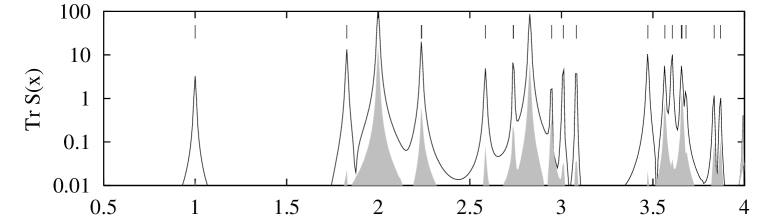
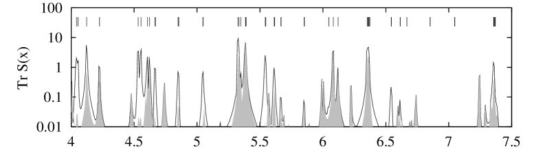
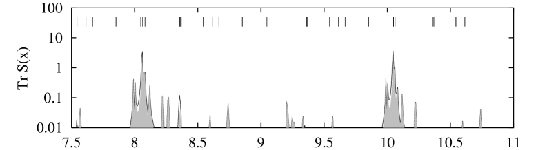
         x

Figure 16: The length spectrum of ${\rm Tr}\,S(k)$ for $a=1$ and $R=0.5$ in the interval ${ka/\pi}=1,\dots,281$ with $\Delta_{k}=\pi/64$. The full line shows the quantum data and the shaded areas represent the error of the leading order semiclassical approximation. The location of the periodic orbits contributing to ${\rm Tr}\,S$ is marked with vertical bars.

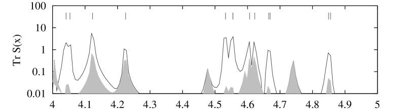
         x

Figure 17: The length spectrum of ${\rm Tr}\,S(k)$ for $a=1$ and $R=0.5$ in the interval ${ka/\pi}=1,\dots,281$. The full line shows the quantum data and the shaded areas represent the error of the standard semiclassical approximation. The location of the unstable periodic orbits contributing to ${\rm Tr}\,S$ is marked with the dotted vertical lines.

4.04157 -0.45E+03	4.05367 0.48E+03	4.12311 0.70E+02	4.22499 0.17E+04
4.53226 0.10E+03	4.55502 0.11E+03	4.60635 0.21E+04	4.62233 0.23E+04
4.66531 0.38E+04	4.66976 0.39E+04	4.84938 0.89E+04	4.85549 0.94E+04

Figure 18: The unstable periodic orbits contributing to ${\rm Tr}\,S(k)$ with lengths in the interval $4\leq L\leq 5$ corresponding to figure 17. Below the figures the length and the stability prefactor of the individual orbits are given.

Now we would like to discuss the semiclassical approximation to ${\rm Tr}\,S$ in more detail. Again we will show that important corrections to the leading order semiclassical result are due to diffraction effects. In figure 16 we display the length spectrum of ${\rm Tr}\,S$, which can be expressed semiclassically in terms of all periodic orbits of the Sinai billiard hitting the section $\Gamma_{\rm S}$ exactly one time. This includes the contributions from the two bouncing ball families present in the Sinai billiard with $R=0.5$ which result in the two most prominent peaks in the spectrum at $x=2$ and $x=2\sqrt{2}$. Most of the other large peaks can be related to isolated unstable periodic orbits as it can be seen from the vertical bars in the upper part of the figures which denote the lengths of all the classical orbits contributing to $S$. The remaining difference between the semiclassical approximation and the quantum data after the leading order contributions from all classical orbits have been included according to the standard Gutzwiller result is displayed using the grey shaded areas. We see that the semiclassical result accounts very well for some of the peaks at small lengths: all the peaks up to $x=4$ are reduced by the subtraction of the semiclassical result by at least a factor of 10 (note the logarithmic scale). The result becomes increasingly worse as the length grows and from $x\approx 7$ the leading order semiclassical theory fails completely.

In order to explain where the deviations come from we have further enlarged the region $4\leq x\leq 5$ in figure 17. There are 12 isolated classical orbits in this interval which are displayed in figure 18. We observe large deviations between the semiclassical result and the quantum data for the orbits with $L=4.12,4.22,4.61$ and $4.62$. These orbits have in common that one of their reflections from the circle is very shallow, i.e. the classical description excluding diffraction effects approaches the limits of its validity. However, unlike the orbits discussed in the context of the spectral density, where a considerable improvement of the semiclassical result could be achieved when the penumbra corrections are taken into account, the orbits of figure 18 are not really well inside penumbra but rather at the border between the illuminated region and the penumbra. Consequently the results of section 2 do not apply. As already mentioned at the end of section 3, a uniform geometric theory of diffraction would be needed in order to correct the contributions from such orbits.

The peaks at $4.47$ and $4.75$ do not correspond to classical orbits but represent the contribution from creeping and “ghost” orbits. $L=2\sqrt{5}a=4.472$ is the length of the first completely shaded bouncing ball family, which does not give a contribution to leading order. However, an important diffraction correction resulting in the observed peak in the length spectrum is due to those orbits in the family which traverse the penumbra.

6.08276 0.15E+03	8.06226 0.26E+03	10.04988 0.41E+03	12.04159 0.58E+03
6.12133 -0.93E+04	8.08221 -0.29E+05	10.06202 -0.67E+05	12.04975 -0.13E+06

Figure 19: Some of the orbits which give rise to the peaks at large x in the length spectrum of ${\rm Tr}\,S$. Below the orbits the length and the dominating eigenvalue of the monodromy matrix are given. Due to diffraction the standard Gutzwiller formula fails to predict the contributions of these orbits correctly.

Finally we turn to the conspicuous peaks in the length spectrum of ${\rm Tr}\,S$ which are located in the vicinity of $x=8,10,12,\dots$ and can be explained by the orbits displayed in figure 19. Below the orbits the length and the dominant eigenvalue of the monodromy matrix are given. The orbits become very unstable as the length increases and the standard Gutzwiller expression fails completely to predict the amplitude of their contribution, which is due to the almost tangent reflection from the circle. Although the penumbra approximation is much better and predicts at least the order of magnitude of the contributions, it is not capable of giving a satisfactory quantitative description and therefore not displayed. While for the shorter orbits the reflection from the circle is not yet inside the penumbra, the problem with the longer orbits is that more and more of the straight segments are close to the circle and need an additional diffraction correction which leads to an increasing error. Moreover additional corrections due to intermittency which were recently derived in [4] may be necessary to predict the amplitudes correctly since the long orbits are very close in phase space to the family bb of bouncing ball orbits transversal to the channel.

5 Frequency of penumbra traversals

The numerical examples of section 4.1 illustrated the success of the theory derived in section 2 to account for the significant penumbra corrections for particular periodic orbits. A natural question would be: how many periodic orbits should be corrected in this way? To answer this question we should consider two factors. First, the borderlines of the penumbra are $k$ dependent and the fraction of phase space occupied by the penumbra is of order $(kL)^{-2/3}$, where $L$ is a typical length of the billiard. This means that the penumbra shrinks to $0$ as $k\rightarrow\infty$. In particular, we can also conclude that any given periodic orbit (that has no exactly tangent segments) will be outside the penumbra for $k$ large enough. The second factor to consider is that in order to quantize the billiard up to a wavenumber $k$ with a resolution of the mean level spacing one needs to consider periodic orbits up to the Heisenberg length $L_{\rm H}\approx kL^{2}$, or, equivalently up to number of bounces $n_{\rm H}\approx kL$. This enhances the chance to visit a given area of phase space as $k$ grows. To obtain the overall effect of these two contradicting trends, let us consider for each periodic orbit $\Delta\equiv\min_{j}|l_{j}-kR|$, where $l_{j}$ is the angular momentum of the $j$th segment of the orbit with respect to the circles center. The orbit traverses the penumbra at least once if $\Delta\mathchar 13614\relax(kR)^{1/3}$. If we assume ergodicity, then each segment of the orbit has an a-priori probability

$$p\approx(kL)^{-2/3}$$ (54)

to traverse the penumbra. Assuming statistical independence of the segments, and homogeneous coverage of phase space by long periodic orbits, the probability that an orbit with $n$ bounces avoids the penumbra is

$$(1-p)^{n}\approx\exp\left[-n(kL)^{-2/3}\right]=\exp\left(-\frac{n}{n_{\rm H}^{2/3}}\right).$$ (55)

Because of the exponential proliferation of periodic orbits, the overwhelming majority of periodic orbits satisfy $n\approx n_{\rm H}$ and thus $n_{\rm H}^{2/3}\mathchar 13614\relax n$. This means according to (55) that in the semiclassical limit most of the periodic orbits traverse the penumbra at least once, and for them the semiclassical approximation fails and should be corrected. To emphasize this point we rephrase our findings about the semiclassical limit in the following way:

• Given a periodic orbit (which is not exactly tangent), its standard semiclassical contribution is recovered for $k$ large enough.

• For a given $k$, most periodic orbits which are shorter than $\approx n_{\rm H}^{2/3}$ are described by the standard semiclassical approximation.

• Although their number grows with $k$, their fraction out of the relevant periodic orbits becomes smaller, and the great majority of periodic orbits are affected by penumbra corrections.

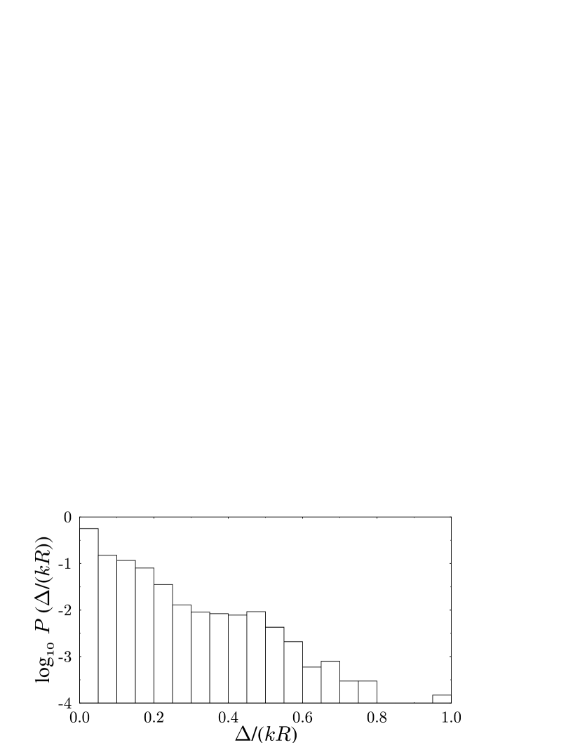
Figure 20: The coarse–grained distribution of $\Delta/(kR)$. Note the logarithmic scale.

To verify these ideas we calculated $\Delta/(kR)$ for all periodic orbits of length up to $10$ of the quarter Sinai billiard. There were $20\,150$ primitive orbits, with total of $320\,002$ segments. The coarse–grained distribution is shown in figure 20. It is sharply peaked near the minimal value $\Delta=0$, which indicates that almost all periodic orbits include a nearly tangent chord, as predicted. To get a quantitative estimate, let us take the Heisenberg length to be the maximal periodic orbit length: $L_{\rm H}=10$. We need to estimate the relevant $k$. We use the definition of the Heisenberg time

$$T_{\rm H}(E)=h\bar{d}(E)\,,$$ (56)

which for billiards can be written as

$$2\pi\bar{d}(k)=L_{\rm H}(k).$$ (57)

If we use the leading order expression for $\bar{d}(k)$ for billiards

$$\bar{d}(k)=\frac{Ak}{2\pi}\,,$$ (58)

where $A$ is the area of the billiard we get

$$k=\frac{L_{\rm H}}{A}\approx 12.4$$ (59)

in our case. The relative phase space area occupied by the penumbra is estimated as

$$p\approx\frac{2(kR)^{\frac{1}{3}}}{kb_{max}}\approx 0.21\,,$$ (60)

where $b_{max}=\sqrt{2}$ is the maximal impact parameter in the billiard. The factor $2$ is due to taking into account impact parameters which are both larger and smaller than $R$. The number of bounces is estimated by

$$n_{\rm H}=\frac{L_{\rm H}}{c}=\frac{L_{\rm H}\gamma}{\pi A}\approx 15\,,$$ (61)

where $c$ is the mean chord and $\gamma$ is the billiards perimeter. Due to the exponential proliferation of orbits, their majority will have a length close to $L_{\rm H}$ and thus $n_{\rm H}$ chords. The probability of such orbits to avoid the penumbra is

$$q=(1-p)^{n_{\rm H}}\approx 0.03$$ (62)

and consequently about $97\%$ of the orbits are expected to traverse the penumbra. The penumbra borders in terms of $\Delta/(kR)$ are estimated as

$$\frac{\Delta}{kR}\leq(kR)^{-\frac{2}{3}}\approx 0.3$$ (63)

which includes according to the numerical data $95.7\%$ of the orbits, in good agreement with the theory.

6 Conclusions

In this paper we have considered the semiclassical quantization of billiard systems. Using asymptotic approximations to the circle Green function we have derived corrections to the standard Gutzwiller formula which account for the quantum diffraction from concave parts of the billiard boundary in the penumbra. This is the nearly tangent parameter region where neither the leading order semiclassical result nor the deep shadow approximation [6, 7] are valid. There are two types of corrections: the first can be expressed in terms of nearly tangent classical periodic orbits (including “ghost” orbits which cut straight through the concave billiard boundary). The contributions from these orbits differ from the Gutzwiller result by a prefactor of the order one, i.e. the correction can be as large as the standard semiclassical amplitude itself. The other type of correction can be expressed in terms of creeping orbits including those with negative creeping angles. Although these orbits are also obtained from the deep shadow approximation, their contribution is different in the penumbra: the amplitude does not decay exponentially in $k$ but only as $k^{-1/6}$ for each creeping segment of the orbit. The appearance of this new type of orbits in the semiclassical quantization formulas raises questions about the structure of the set of all creeping orbits, e.g. how they can be computed using an extremum principle together with a code and if there is a one to one correspondence between the nearly tangent classical orbits and the creeping counterparts by which they have to be replaced in the case of penumbra diffraction. Although we have some preliminary results for the Sinai billiard, the answer to these questions is beyond the scope of the present paper.

The derived corrections to the standard Gutzwiller result have been tested in both, the integrable annular billiard and the chaotic Sinai billiard. The success of the theory was obvious as long as the orbits under consideration were indeed well inside the penumbra region.

In the case of the Sinai billiard we have used beside the length spectrum obtained from the set of billiard eigenvalues also an alternative method of spectral analysis which is based on the scattering approach to quantization. Here discrete length spectra are directly obtained from the total phase or the traces of the involved S-matrix which has the advantage that only limited subsets of periodic orbits contribute. The resulting sparse spectrum is particularly well suited to observe deviations from the standard Gutzwiller result and we could in this way check the quality of the penumbra and the deep shadow approximation to a high precision.

The importance of penumbra diffraction corrections becomes obvious if one estimates the number of orbits which are affected by them. It turns out that the amplitudes of most of the orbits contributing to the spectrum up to some fixed value $k$ must be corrected. In view of this fact it would certainly be desirable to further extend the results which we presented in this paper to the parameter regions, where none of the so far known expressions is sufficiently accurate.

Appendix A The circle Green function with Neumann and mixed boundary conditions

The different approximations to the circle Green function are found in a manner similar to section 2.1 when homogeneous boundary conditions are imposed on the circle. In this appendix we give the modifications to the expressions derived in section 2.1 for this case. Equations (13-14) are still the starting point for all calculations, and the boundary conditions affect only the scattering matrix $S_{l}(kR)$.

For Neumann boundary conditions ($\partial_{\bf\hat{n}}\psi({\bf r})=0$) the scattering matrix is given by

$$S_{l}(kR)=-\frac{H_{l}^{-^{\prime}}(kR)}{H_{l}^{+^{\prime}}(kR)}\,.$$ (A1)

In the lit region, $G_{\rm d}({\bf r},{\bf r^{\prime}})$ (15), the contribution of the direct path, is unaffected, while the contribution of the reflected path $G_{\rm r}({\bf r},{\bf r^{\prime}})$ (16) is multiplied by $-1$. In the deep shadow region, the contribution of the creeping path $G_{\rm c}^{(0)}({\bf r},{\bf r^{\prime}})$ is still given by (19-20), but with different poles $l_{n}$ and residues $r_{n}$. The poles are given by (17), where in this case $x_{n}$ are the zeros of ${\rm Ai}^{\prime}(x)$. The residues are given by

$$r_{n}=\frac{{\mathrm{e}}^{-{\mathrm{i}}\pi/6}}{2\pi x_{n}{\rm Ai}(-x_{n})^{2}}\left(\frac{kR}{2}\right)^{\frac{1}{3}}\,.$$ (A2)

In the penumbra the contribution of the direct path $G_{\rm d}({\bf r},{\bf r^{\prime}})$ (26) is unaffected by the boundary conditions. The constant $c$ in the contribution from the tangent path $G_{\rm g}({\bf r},{\bf r^{\prime}})$ (31) is now given by

$$c=-\frac{1}{2^{1/3}}\int_{-\infty}^{0}{\rm d}x\,\frac{{\rm Ai}^{\prime}(x{\mathrm{e}}^{-2\pi{\mathrm{i}}/3})}{{\rm Ai}^{\prime}(x{\mathrm{e}}^{2\pi{\mathrm{i}}/3})}+\frac{{\mathrm{e}}^{-2\pi{\mathrm{i}}/3}}{2^{1/3}}\int_{0}^{\infty}{\rm d}x\,\frac{{\rm Ai}^{\prime}(x)}{{\rm Ai}^{\prime}(x{\mathrm{e}}^{2\pi{\mathrm{i}}/3})}\,.$$ (A3)

The first term is again the complex conjugate of the second [25], and by a numerical integration over the second term we have

$$c\approx-0.864251443481\,.$$ (A4)

We now consider the general case of mixed boundary conditions ($\kappa\psi({\bf r})+\partial\hat{n}\psi({\bf r})=0$). Neumann boundary conditions are the case of $\kappa=0$, and Dirichlet boundary conditions are the limit $\kappa\rightarrow\infty$. The semiclassical quantization for mixed boundary conditions is considered in [30]. The scattering matrix is given by

$$S_{l}(kR)=-\frac{\kappa H_{l}^{-}(kR)-kH_{l}^{-^{\prime}}(kR)}{\kappa H_{l}^{+}(kR)-kH_{l}^{+^{\prime}}(kR)}\,.$$ (A5)

In the lit region $G_{\rm d}({\bf r},{\bf r^{\prime}})$ (15) is again unaffected. The contribution of the reflected path, $G_{\rm r}({\bf r},{\bf r^{\prime}})$ (16) is multiplied by a phase ${\mathrm{e}}^{{\mathrm{i}}\phi}$, where $\phi$ is given [30] by

$$\phi=2\arctan\left(\frac{k}{\kappa}\cos\theta\right)\,.$$ (A6)

Note that for $\kappa\rightarrow\infty$ (Dirichlet) $\phi=0$, and for $\kappa=0$ (Neumann) $\phi=\pi$. The poles $l_{n}$ for the contribution of the creeping path $G_{\rm c}^{(0)}({\bf r},{\bf r^{\prime}})$ (19-20) in the deep shadow region are still given by (17), where in this case $x_{n}$ are the solutions of

$$\frac{{\rm Ai}^{\prime}(-x)}{{\rm Ai}(-x)}={\mathrm{e}}^{{\mathrm{i}}\pi/3}\frac{\kappa}{k}\left(\frac{kR}{2}\right)^{\frac{1}{3}}\,.$$ (A7)

The residues are given by

$$r_{n}=\frac{{\mathrm{e}}^{-i\pi/6}}{2\pi\left[{\rm Ai}^{\prime}(-x_{n})^{2}+x_{n}{\rm Ai}(-x_{n})^{2}\right]}\left(\frac{kR}{2}\right)^{\frac{1}{3}}\,.$$ (A8)

In the penumbra $G_{\rm d}({\bf r},{\bf r^{\prime}})$ (26) is again unaffected. The constant $c$ in $G_{\rm g}({\bf r},{\bf r^{\prime}})$ (31) must be replaced by the $k$-dependent expression

$$c\left(\frac{\kappa}{k}\left[\frac{kR}{2}\right]^{\frac{1}{3}}\right)\,.$$ (A9)

After some manipulations $c(z)$ is given in a form convenient for numerical integration by

$$c(z)=\frac{1}{2^{1/3}}\int_{0}^{\infty}{\rm d}x\,\frac{z{\rm Ai}(x)+{\mathrm{e}}^{-2\pi{\mathrm{i}}/3}{\rm Ai}^{\prime}(x)}{z{\rm Ai}({\mathrm{e}}^{-2\pi{\mathrm{i}}/3}x)+{\mathrm{e}}^{2\pi{\mathrm{i}}/3}{\rm Ai}^{\prime}({\mathrm{e}}^{-2\pi{\mathrm{i}}/3}x)}$$

$$+\frac{1}{2^{1/3}}\int_{0}^{\infty}{\rm d}x\,\frac{z{\rm Ai}(x)+{\rm Ai}^{\prime}(x)}{z{\rm Ai}({\mathrm{e}}^{2\pi{\mathrm{i}}/3}x)+{\mathrm{e}}^{2\pi{\mathrm{i}}/3}{\rm Ai}^{\prime}({\mathrm{e}}^{2\pi{\mathrm{i}}/3}x)}\,.$$ (A10)

For some applications it is convenient to express mixed boundary conditions as $b\cos\alpha\psi({\bf r})+\sin\alpha\partial_{\hat{n}}\psi({\bf r})=0$. The parameter $\alpha$ interpolates between Dirichlet ($\alpha=0$) and Neumann ($\alpha=\pi/2$) boundary conditions. In [30] the derivative

$$\left.\frac{\partial}{\partial\alpha}d(k;b,\alpha)\right|_{\alpha=0}$$ (A11)

is introduced as a tool for analyzing the spectrum of the Sinai billiard. It was conjectured there that the derivative of tangent contributions should semiclassically vanish. Using (A10) we find that

$$\left.\frac{{\mathrm{d}}}{{\mathrm{d}}\alpha}c\left(\frac{b}{k}\left[\frac{kR}{2}\right]^{\frac{1}{3}}\cot\alpha\right)\right|_{\alpha=0}={\mathrm{e}}^{2\pi{\mathrm{i}}/3}\frac{k}{b}\frac{1}{(kR)^{1/3}}\,,$$ (A12)

which together with (47), (50) and (51) indeed gives a contribution $\mathop{\mathrm{O}}\nolimits(k^{-1/2})$ smaller than for a standard unstable periodic orbit.

Appendix B Calculation of direct contributions

In this appendix we calculate the purely “direct” contributions to $d_{\rm bb,1}(k)$ and $d_{\rm bb,2}(k)$ that appear in section 4.1.1. The purpose is to find genuine diffractive (penumbra) contributions beyond the semiclassical ones [2]. There is an inherent difficulty in this problem, since diffractive effects are localized near the circle, while the bouncing ball family is more global and covers a considerable volume of configuration space. In the lack on a uniform approximation for the direct contribution $G_{\rm d}$, it is natural to consider a splitting of the integration region into “near” and “far” regions, using the appropriate expressions in each region. However, in our case it is not completely clear what is the correct splitting, and what is the correct transition between the penumbra and the illuminated and shadowed regions. Thus we choose to use the penumbra approximation of $G_{\rm d}$ for the whole integration region, and after performing the calculation to consider more closely the origin of corrections, if any.

To get $d_{\rm bb,1}^{\rm d}(k)$ we substitute in equation (44) the explicit form of $G_{\rm d}$ (equation (26)), and to leading order in $k$ we have

$$d_{\rm bb,1}^{\rm d}(k)=\frac{\sqrt{2kL}}{\pi^{\frac{3}{2}}}\Im\left\{{\mathrm{e}}^{{\mathrm{i}}kL+{\mathrm{i}}\frac{\pi}{4}}\int_{0}^{\frac{L}{2}}\tilde{F}\left(2\sqrt{\frac{k}{\pi L}}(R-x)\right){\rm d}x\right\}\,,$$ (B13)

where we denoted $\tilde{F}(x)\equiv[F(\infty)-F(x)]/\sqrt{2{\mathrm{i}}}$. The integral is evaluated by using the indefinite integral of the Fresnel function

$$I_{1}(t)\equiv\int^{t}\tilde{F}(t^{\prime}){\rm d}t^{\prime}=t\tilde{F}(t)-\frac{1}{\pi}\sqrt{\frac{{\mathrm{i}}}{2}}{\mathrm{e}}^{{\mathrm{i}}\frac{\pi}{2}t^{2}}.$$ (B14)

It can be simplified, if we consider the asymptotic approximation of the Fresnel function for $|t|\gg 1$:

$$F(t)=F(\infty)\ {\rm sign}(t)-\frac{{\mathrm{i}}}{\pi t}{\mathrm{e}}^{{\mathrm{i}}\frac{\pi}{2}t^{2}}+\mathop{\mathrm{O}}\nolimits(|t|^{-3}).$$ (B15)

Combining (B15) with (B14) we get

$$I_{1}(t)\approx\frac{1-{\rm sign}(t)}{2}t=\left\{\begin{array}[]{cc}t&t<0\\ 0&t>0\end{array}\right.\,.$$ (B16)

Thus finally

$$d_{\rm bb,1}^{\rm d}(k)=\frac{(L-2R)\sqrt{kL}}{\sqrt{2}\pi^{\frac{3}{2}}}\cos\left(kL-\frac{\pi}{4}\right)+\mathop{\mathrm{O}}\nolimits(k^{-\frac{1}{2}})\,.$$ (B17)

This recovers the semiclassical contribution of the bouncing balls [2]. There are no diffraction corrections to $d_{\rm bb,1}^{\rm d}(k)$ that are larger than the semiclassical error of the bouncing ball contributions. We emphasize that the asymptotic approximation of $F(t)$ was invoked after the integration was performed. This is completely justified, because the argument of both limits is $\mathop{\mathrm{O}}\nolimits(k^{\frac{1}{2}})\gg 1$. Replacing the integrand with the asymptotic form would be unjustified, since the interesting region near the circle is not asymptotic.

For the double repetition the situation is more interesting. To leading order in $k$ we have

$$d_{\rm bb,2}^{\rm dd}(k)=\frac{\sqrt{kL}}{\pi^{\frac{3}{2}}}\Im\left\{{\mathrm{e}}^{2{\mathrm{i}}kL+{\mathrm{i}}\frac{\pi}{4}}\int_{0}^{\frac{L}{2}}\tilde{F}^{2}\left(2\sqrt{\frac{k}{\pi L}}(R-x)\right){\rm d}x\right\}.$$ (B18)

The relevant integral is

$$I_{2}(t)\equiv\int^{t}\tilde{F}^{2}(t^{\prime}){\rm d}t^{\prime}=t\tilde{F}^{2}(t)-\frac{\sqrt{2{\mathrm{i}}}}{\pi}\tilde{F}(t){\mathrm{e}}^{{\mathrm{i}}\frac{\pi}{2}t^{2}}-\frac{1}{\sqrt{2}\pi}F(\sqrt{2}t)$$ (B19)

$$\hbox to0.0pt{\hss${}\approx{}$}t\left[\frac{1-{\rm sign}(t)}{2}\right]-\frac{\sqrt{{\mathrm{i}}}}{2\pi}{\rm sign}(t)=\left\{\begin{array}[]{rc}t+\sqrt{{\mathrm{i}}}/(2\pi)&t<0\\ -\sqrt{{\mathrm{i}}}/(2\pi)&t>0\end{array}\right.\,,$$ (B22)

where the last line was obtained using the asymptotic approximation of $F(t)$. Equation (B22) indicates, that in the lit region ($t<0,|t|\gg 1$) we obtain a linear contribution, together with a constant that comes from the integration near $t\approx 0$. In the shadowed region we have only a constant contribution from the $t\approx 0$ region. Inserting (B22) into (B18) we get

$$d_{\rm bb,2}^{\rm dd}(k)=\frac{\sqrt{kL}}{\pi^{\frac{3}{2}}}\left(\frac{L}{2}-R\right)\cos\left(2kL-\frac{\pi}{4}\right)-\frac{L}{2\pi^{2}}\cos(2kL)+\mathop{\mathrm{O}}\nolimits(k^{-\frac{1}{2}}).$$ (B23)

Thus, in addition to the semiclassical contribution due to the bouncing balls, we obtain a genuine diffractive contribution. It is $\mathop{\mathrm{O}}\nolimits(k^{0})$ which is the same as for an unstable periodic orbit and therefore must be retained. The explicit form of $I_{2}(t)$ in (B22) indicates that indeed this diffraction contribution is obtained from the region near the circle and is not a result of a more global effect.

References

References

- [1] M. V. Berry. Quantizing a classically ergodic system: Sinai billiard and the KKR method. Ann. Phys., 131:163–216, 1981.
- [2] M. Sieber, U. Smilansky, S. C. Creagh, and R. G. Littlejohn. Non-generic spectral statistics in the quantized stadium billiard. J. Phys. A, 26:6217–6230, 1993.
- [3] V. F. Lazutkin. KAM Theory and Semiclassical Approximations to Eigenfunctions. Springer, Berlin, 1993.
- [4] G. Tanner. How chaotic is the stadium billiard ? A semiclassical analysis. to be published.
- [5] M. C. Gutzwiller. Periodic orbits and classical quantization conditions. J. Math. Phys., 12:343–358, 1971.
- [6] B. R. Levy and J. B. Keller. Diffraction by a smooth object. Comm. Pure Appl. Math., 12:159–209, 1959.
- [7] G. Vattay, A. Wirzba, and P. E. Rosenqvist. Periodic orbit theory of diffraction. Phys. Rev. Lett., 73:2304–2307, 1994.
- [8] H. Primack, H. Schanz, U. Smilansky, and I. Ussishkin. The rôle of diffraction in the quantization of dispersing billiards. Phys. Rev. Lett., 76:1615–1619, 1996.
- [9] E. Doron and U. Smilansky. Semiclassical quantization of chaotic billiards: A scattering theory approach. Nonlinearity, 5:1055–1084, 1992.
- [10] C. Rouvinez and U. Smilansky. A scattering approach to the quantization of Hamiltonians in 2 dimensions – application to the wedge billiard. J. Phys. A, 28:77–104, 1995.
- [11] H. Schanz and U. Smilansky. Quantization of Sinai’s billiard – A scattering approach. Chaos, Solitons Fractals, 5:1289–1309, 1995.
- [12] U. Smilansky. Semiclassical quantization of chaotic billiards – A scattering approach. In E. Akkermans, G. Montambaux, and J. L. Pichard, editors, Mesoscopic Quantum Physics, Les Houches Summer School Sessions LXI, Amsterdam, 1996. North-Holland.
- [13] K. G. Andersson and R. B. Melrose. The propagation of singularities along gliding rays. Inventiones math., 41:197–232, 1977.
- [14] E. B. Bogomolny. Semiclassical quantization of multidimensional systems. Nonlinearity, 5:805–866, 1992.
- [15] M. C. Gutzwiller. Poincaré surface of section and quantum scattering. Chaos, 3:591–599, 1993.
- [16] T. Prosen. General quantum surface-of-section method. J. Phys. A, 28:4133–4155, 1995.
- [17] M. Sh. Birman and D. R. Yafaev. The spectral shift function. The work of M. G. Krein and its further development. St. Petersburg Math. J., 4:833–870, 1993.
- [18] P. Gaspard and S. A. Rice. Semiclassical quantization of the scattering from a classically chaotic repellor. J. Chem. Phys., 90:2242, 1989.
- [19] P. Gaspard. Scattering and resonances: Classical and quantum dynamics. In G. Casati, I. Guarneri, and U. Smilansky, editors, Proceedings of the International School of Physics “Enrico Fermi”, Course CXIX, pages 307–383, Amsterdam, 1993. North-Holland.
- [20] U. Smilansky and I. Ussishkin. The smooth spectral counting function and the total phase shift for quantum billiards. J. Phys. A: Math. Gen., 26:2587–2597, 1996.
- [21] H. P. Baltes and E. R. Hilf. Spectra of Finite Systems. Bibliographisches Institut, Mannheim, 1976.
- [22] H. M. Nussenzveig. High-frequency scattering by an impenetrable sphere. Ann. Phys., 34:23–95, 1965.
- [23] D. Alonso and P. Gaspard. expansion for the periodic orbit quantization of chaotic systems. Chaos, 3:601–612, 1993.
- [24] M. Abramowitz and I. A. Stegun, editors. Handbook of Mathematical Functions. Dover, New York, 1965.
- [25] S. I. Rubinow and T. T. Wu. First correction to the geometric-optics scattering cross section from cylinders and spheres. J. Appl. Phys., 27:1032–1039, 1956.
- [26] L. A. Bunimovich. Variational principle for periodic trajectories of hyperbolic billiards. Chaos, 5:349–355, 1995.
- [27] M. Sieber. The Hyperbola Billiard: A Model for the Semiclassical Quantization of Chaotic Systems. PhD thesis, University of Hamburg, 1991. DESY report 91–030.
- [28] E. Doron and U. Smilansky. Chaotic spectroscopy. Phys. Rev. Lett., 68:1255–1258, 1992.
- [29] W. H. Press. Numerical Recipes in FORTRAN. Cambridge University Press, Cambridge, 1994.
- [30] M. Sieber, H. Primack, U. Smilansky, I. Ussishkin, and H. Schanz. Semiclassical quantization of billiards with mixed boundary conditions. J. Phys. A: Math. Gen., 28:5041–5078, 1995.