ULM–TP/96-4
November 1996

Semiclassical Transition from an Elliptical

to an Oval Billiard

Martin Sieber^1,2

¹ Division de Physique Théorique, Institut de Physique Nucléaire, F-91406 Orsay Cedex, France
² Abteilung Theoretische Physik, Universität Ulm, D-89069 Ulm, Germany

Abstract

Semiclassical approximations often involve the use of stationary phase approximations. This method can be applied when $\hbar$ is small in comparison to relevant actions or action differences in the corresponding classical system. In many situations, however, action differences can be arbitrarily small and then uniform approximations are more appropriate. In the present paper we examine different uniform approximations for describing the spectra of integrable systems and systems with mixed phase space. This is done on the example of two billiard systems, an elliptical billiard and a deformation of it, an oval billiard. We derive a trace formula for the ellipse which involves a uniform approximation for the Maslov phases near the separatrix, and a uniform approximation for tori of periodic orbits close to a bifurcation. We then examine how the trace formula is modified when the ellipse is deformed into an oval. This involves uniform approximations for the break-up of tori and uniform approximations for bifurcations of periodic orbits. Relations between different uniform approximations are discussed.

PACS numbers:
03.65.Ge   Solutions of wave equations: bound states.
03.65.Sq   Semiclassical theories and applications.
05.45.+b   Theory and models of chaotic systems.

Submitted to Journal of Physics A

1 Introduction

Semiclassical trace formulas are important tools for analyzing spectra of quantum systems. They have found a wide range of applications in recent years (see for example [1, 2, 3]). Trace formulas have been derived for integrable and chaotic systems when periodic orbits lie on tori in phase space or are isolated [4, 5, 6, 7, 8]. Families of orbits in systems with more general symmetries have also been treated [9, 10].

Most systems, however, are neither integrable nor chaotic, but have a phase space which is intricately divided into regular and chaotic regions. In these systems there exist classical structures on all scales, and neighbouring periodic orbits can have arbitrarily small action differences. For the semiclassical approximation this has the consequence that in many cases stationary phase approximations cannot be applied since they rely on the fact that action differences of periodic orbits are large in comparison to $\hbar$. Instead one has to use approximations which are uniformly valid in two small parameters, $\hbar$ and $\varepsilon$, where $\varepsilon$ describes the separation of neighbouring periodic orbits.

A typical situation where small action differences of periodic orbits occur is near bifurcations of periodic orbits. Bifurcations are a ubiquitous phenomenon in mixed systems. They occur any time the stability angle of a stable orbit is a rational multiple of $2\pi$. If, for example, one changes an external parameter of a system by an arbitrarily small but finite amount (or the energy in a generic system), then in general an infinite number of bifurcations occur, most of them for long periodic orbits.

Bifurcations occur in different forms, but the number of generic forms in two-dimensional systems is finite. They were classified by Meyer [11] and Bruno [12, 13]. Their form depends on the repetition number $m$ of an orbit that bifurcates. The semiclassical treatment of these generic bifurcations was investigated by Ozorio de Almeida and Hannay [14]. They derived contributions to the trace formula from periodic orbits near bifurcations in terms of standard diffraction catastrophe integrals. These approximations have for example been applied for treating tangent bifurcations and pitchfork bifurcations [15, 16]. For the largest class of bifurcations with $m>4$ the results of Ozorio de Almeida and Hannay were extended in [17] by including higher order terms in the normal form expansion for the bifurcation. In this way a uniform approximation was obtained which interpolates over the regime from the bifurcation up to regions where Gutzwiller’s approximation can be applied.

Another situation in which small action differences occur is in the quasi-integrable regime, i. e. for small perturbations of integrable systems. Due to the perturbation all rational tori of the integrable system break up into a finite number of periodic orbits which have small action differences when the perturbation is small. Ozorio de Almeida derived a uniform approximation which is valid if the splitting of the orbits is small [18]. A formula for the break-up of families of orbits due to more general symmetries was derived by Creagh [19]. Tomsovic, Grinberg and Ullmo extended the result of Ozorio de Almeida and obtained a uniform approximation which interpolates between the torus contribution and Gutzwiller’s approximation [20, 21].

Small action differences of neighbouring periodic orbits can occur also in integrable systems, since bifurcations of periodic orbits can occur also there. These bifurcations do not belong to the class of generic bifurcations, since they result in the appearance of whole new tori of periodic orbits. A uniform approximation for the contributions of tori that result from the bifurcation of a stable orbit was derived by Berry and Tabor [6] and Richens [22].

The present paper contains an investigation and discussion of the various concepts which are mentioned above. This is done on the example of two billiard systems, an ellipse and a deformation of it, an oval. The classical motion in an ellipse is integrable and has several characteristic properties. There is a separatrix which separates two kinds of motion, around the two foci and between the two foci. Furthermore, in addition to the usual tori of periodic orbits there are also two isolated periodic orbits in the ellipse (and their repetitions), one stable and one unstable. When the eccentricity of the ellipse is increased, then new tori of periodic orbits arise through bifurcations of the stable orbit and its repetitions. All these classical properties have an influence on the semiclassical approximation. After a brief review of the classical and quantum mechanics in the ellipse we discuss the semiclassical EBK-quantization for the ellipse. Near the separatrix this quantization condition has to be modified by a (non-integer) uniform approximation for the Maslov index, since this index is discontinuous at the separatrix which leads to ambiguities and inaccuracies in the semiclassical quantization [23, 24]. From this modified EBK-quantization condition we derive a trace formula for the ellipse. We show in detail, how the contributions of regular tori of orbits, of tori near bifurcations, of the isolated periodic orbits and the area and perimeter contributions can be obtained from the modified EBK-quantization conditions. We close this section with a numerical examination of the trace formula.

We then examine an oval-shaped billiard which can be considered as a deformation of an ellipse. We investigate how the semiclassical approximation for the ellipse is changed when the ellipse is deformed into the oval. Due to this perturbation all tori of periodic orbits break up into a finite number of orbits. When the tori are not close to a bifurcation then the uniform approximation for the break-up of tori can be applied. For tori near bifurcations one has to use a different approximation. It will be shown that the (slightly modified) uniform approximations for generic bifurcations describe also the break-up of the tori near bifurcations. We present a detailed numerical examination of semiclassical approximations in the oval, and we discuss the relations between different uniform approximations that are used in this paper.

2 The elliptical billiard

We discuss in this section various properties of the elliptical billiard. This is an integrable billiard system whose boundary is defined by

$$\frac{x^{2}}{a^{2}}+\frac{y^{2}}{b^{2}}=1\;,$$ (1)

where $a$ and $b<a$ are the lengths of the semi-major and semi-minor axis, respectively. The ellipse has two focal points with coordinates $(\pm c,0)$, where $c=\sqrt{a^{2}-b^{2}}$, and its eccentricity is defined by $e=c/a$. The billiard area is $A=\pi ab$ and its perimeter is $L=4a\mbox{E}(e)$ where $\mbox{E}(\kappa)$ is the complete elliptic integral of the second kind [25] (see Eq. (16) below).

The classical properties in the elliptical billiard have been investigated under different view points. This includes the treatment of the action-angle variables [26], the caustics of the classical motion [26, 27], Poncelet’s theorem [28, 29], the billiard map [30, 31], and the periodic orbits [29, 32, 33]. A treatment of the Schrödinger equation for the elliptical billiard can be found in [34]. In the following we briefly review classical and quantum properties of the elliptical billiard because they are used for the semiclassical approximation. We then discuss the EBK-quantization for the billiard and a uniform extension of it, and we derive a trace formula in terms of the periodic orbits of the system.

2.1 Classical mechanics of the elliptical billiard

The classical motion of a particle in an elliptical billiard is conveniently described in elliptical coordinates

$$x = c\,\cosh u\,\cos v$$

$$y = c\,\sinh u\,\sin v\;,$$ (2)

where $u$ is restricted to $0\leq u\leq\mbox{arctanh}(b/a)$ and $v$ is a periodic coordinate with period $2\pi$. In terms of these coordinates the Lagrangian has the form (with mass $m=1/2$)

$$L=\frac{c^{2}}{4}(\cosh^{2}u-\cos^{2}v)(\dot{u}^{2}+\dot{v}^{2})\;,$$ (3)

the canonical momenta are given by

$$p_{u} = \frac{\partial L}{\partial\dot{u}}=\frac{c^{2}}{2}\dot{u}\,(\cosh^{2}u-\cos^{2}v)$$

$$p_{v} = \frac{\partial L}{\partial\dot{v}}=\frac{c^{2}}{2}\dot{v}\,(\cosh^{2}u-\cos^{2}v)\;,$$ (4)

and the Hamiltonian is

$$H=\frac{p_{u}^{2}+p_{v}^{2}}{c^{2}(\cosh^{2}u-\cos^{2}v)}\;.$$ (5)

The two conserved quantities of the system are the energy and the product $L_{1}L_{2}$ of the two angular momenta about the two foci

$$L_{1}L_{2}=\frac{p_{v}^{2}\sinh^{2}u-p_{u}^{2}\sin^{2}v}{\cosh^{2}u-\cos^{2}v}\;.$$ (6)

It is more convenient to use instead of $L_{1}L_{2}$ another conserved quantity which is energy independent and is determined by the geometrical properties of a trajectory only. This is $\alpha=L_{1}L_{2}/E$ whose values are restricted to the range $b^{2}\geq\alpha\geq-c^{2}$. The upper limit $\alpha=b^{2}$ corresponds to the motion along the boundary and the lower limit $\alpha=-c^{2}$ corresponds to the motion along the minor axis.

In terms of $E$ and $\alpha$ the canonical momenta are given by

$$p_{u}^{2} = E(c^{2}\sinh^{2}u-\alpha)$$

$$p_{v}^{2} = E(c^{2}\sin^{2}v+\alpha)\;.$$ (7)

There are two different kinds of motion in the ellipse depending on the sign of $\alpha$. For $0<\alpha\leq b^{2}$ the trajectories have a caustic in form of a confocal ellipse with semi-minor axis $b^{\prime}=\sqrt{\alpha}$. The motion goes around the two focal points and is composed of a libration in the coordinate $u$ and a rotation in the coordinate $v$. For $-c^{2}\leq\alpha<0$ the caustic of the motion is a confocal hyperbola with semi-conjugate axis $b^{\prime}=\sqrt{-\alpha}$ and semi-transverse axis $a^{\prime}=\sqrt{c^{2}+\alpha}$. The motion is composed of a libration in the coordinate $u$ and a libration in the coordinate $v$, and the trajectories cross the $x$-axis always between the two focal points. Both kinds of motions are separated by a separatrix which consists of orbits with $\alpha=0$ that go through the focal points of the ellipse.

The periodic orbits of the elliptical billiard can be determined by introducing action-angle variables. The actions are given by

$$I_{u} = \frac{1}{2\pi}\oint\!p_{u}\,\mbox{d}u=\frac{\sqrt{E}}{\pi}\int_{u_{0}}^{u_{1}}\!\mbox{d}u\,\sqrt{c^{2}\sinh^{2}u-\alpha}$$

$$I_{v} = \frac{1}{2\pi}\oint\!p_{v}\,\mbox{d}v=\frac{2\sqrt{E}}{\pi}\int_{v_{0}}^{v_{1}}\!\mbox{d}v\,\sqrt{c^{2}\sin^{2}v+\alpha}\;,$$ (8)

where

$$\begin{array}[]{lllll}\displaystyle\mbox{for}\;\alpha>0:&\displaystyle u_{0}=\mbox{arcsinh}\frac{b^{\prime}}{c}\,,&\displaystyle u_{1}=\mbox{arcsinh}\frac{b}{c}\,,&\displaystyle v_{0}=0\,,&\displaystyle v_{1}=\frac{\pi}{2}\,,\\[6.0pt] \displaystyle\mbox{for}\;\alpha<0:&\displaystyle u_{0}=0\,,&\displaystyle u_{1}=\mbox{arcsinh}\frac{b}{c}\,,&\displaystyle v_{0}=\arcsin\frac{b^{\prime}}{c}\,,&\displaystyle v_{1}=\frac{\pi}{2}\,,\end{array}$$ (9)

and $b^{\prime}=\sqrt{|\alpha|}$. We choose here a definition of $I_{u}$ which is actually the action for only half a cycle if $\alpha<0$. The reason is that otherwise $I_{u}$ is discontinuous if $\alpha$ changes sign. We remark that the actions in a half-ellipse which is cut along the $x$-axis have the values given by Eqs. (2.1) and (9).

The integrations in (2.1) yield

$$I_{u} = \left\{\begin{array}[]{ll}\displaystyle\frac{\sqrt{E}}{\pi}\left[\frac{a}{b}\sqrt{b^{2}-\alpha}-\frac{c}{\kappa}\,\mbox{E}(\arcsin\sqrt{\frac{b^{2}-\alpha}{b^{2}}},\kappa)\right]&\mbox{for}\;\alpha>0\\[6.0pt] \displaystyle\frac{\sqrt{E}}{\pi}\left[\frac{ab}{\sqrt{b^{2}-\alpha}}-\frac{\alpha}{c}\,\mbox{F}(\arcsin\sqrt{\frac{b^{2}}{b^{2}-\alpha}},\frac{1}{\kappa})-c\,\mbox{E}(\arcsin\sqrt{\frac{b^{2}}{b^{2}-\alpha}},\frac{1}{\kappa})\right]&\mbox{for}\;\alpha<0\end{array}\right.$$ (12)

$$I_{v} = \left\{\begin{array}[]{ll}\displaystyle\frac{2\sqrt{E}}{\pi}\,\frac{c}{\kappa}\,\mbox{E}(\frac{\pi}{2},\kappa)&\phantom{blablablablablablablablablablabla}\mbox{for}\;\alpha>0\\[6.0pt] \displaystyle\frac{2\sqrt{E}}{\pi}\left[\frac{\alpha}{c}\,\mbox{F}(\frac{\pi}{2},\frac{1}{\kappa})+c\,\mbox{E}(\frac{\pi}{2},\frac{1}{\kappa})\right]&\phantom{blablablablablablablablablablabla}\mbox{for}\;\alpha<0\;,\end{array}\right.$$ (15)

where $\kappa=c/a^{\prime}=c/\sqrt{c^{2}+\alpha}$, and the functions

$$\mbox{F}(\varphi,\kappa)=\int_{0}^{\varphi}\!\frac{\mbox{d}\alpha}{\sqrt{1-\kappa^{2}\sin^{2}\alpha}}\;,\hskip 21.52771pt\;\mbox{E}(\varphi,\kappa)=\int_{0}^{\varphi}\!\sqrt{1-\kappa^{2}\sin^{2}\alpha}\,\mbox{d}\alpha\;,$$ (16)

are the elliptic integrals of the first and second kind [25]. The quantity $\kappa$ is called the modulus of the elliptic integrals. The corresponding complete elliptic integrals are denoted by $\mbox{E}(\kappa)=\mbox{E}(\pi/2,\kappa)$ and $\mbox{K}(\kappa)=\mbox{F}(\pi/2,\kappa)$.

The tori of periodic orbits of the elliptical billiard are determined by the condition that the quotient of the angular frequencies $\omega_{u}$ and $\omega_{v}$ is rational:

$$\frac{\omega_{u}}{\omega_{v}}=\frac{\left.\frac{\partial E}{\partial I_{u}}\right|_{I_{v}}}{\left.\frac{\partial E}{\partial I_{v}}\right|_{I_{u}}}=-\left.\frac{\partial I_{v}}{\partial I_{u}}\right|_{E}=-\frac{\left.\frac{\partial I_{v}}{\partial\alpha}\right|_{E}}{\left.\frac{\partial I_{u}}{\partial\alpha}\right|_{E}}=\frac{n}{m}\;,$$ (17)

and with

$$\left.\frac{\partial I_{u}}{\partial\alpha}\right|_{E} = \left\{\begin{array}[]{ll}\displaystyle-\frac{\sqrt{E}\kappa}{2\pi c}\,\mbox{F}\left(\arcsin\sqrt{\frac{b^{2}-\alpha}{b^{2}}},\kappa\right)&\mbox{for}\;\alpha>0\\[8.0pt] \displaystyle-\frac{\sqrt{E}}{2\pi c}\,\mbox{F}\left(\arcsin\sqrt{\frac{b^{2}}{b^{2}-\alpha}},\frac{1}{\kappa}\right)&\mbox{for}\;\alpha<0\end{array}\right.$$ (20)

$$\left.\frac{\partial I_{v}}{\partial\alpha}\right|_{E} = \left\{\begin{array}[]{ll}\displaystyle\frac{\kappa\sqrt{E}}{\pi c}\,\mbox{F}\left(\frac{\pi}{2},\kappa\right)&\hskip 81.8053pt\mbox{for}\;\alpha>0\\[8.0pt] \displaystyle\frac{\sqrt{E}}{\pi c}\,\mbox{F}\left(\frac{\pi}{2},\frac{1}{\kappa}\right)&\hskip 81.8053pt\mbox{for}\;\alpha<0\;,\end{array}\right.$$ (23)

one obtains the conditions for periodic orbits. We will consider in the following the cases $\alpha>0$ and $\alpha<0$ separately.

The case $\alpha>0$:

The condition for periodic orbits is

$$\mbox{F}(\arcsin\sqrt{\frac{b^{2}-\alpha}{b^{2}}},\kappa)=\frac{2m}{n}\,\mbox{F}(\frac{\pi}{2},\kappa)=\frac{2m}{n}\,\mbox{K}(\kappa)\;.$$ (24)

This equation has a solution for all $n=3,4,\dots$ and $1\leq m<n/2$, and the integers $n$ and $m$ are the number of reflections of an orbit and its rotation number, respectively. Eq. (24) determines the value of $\alpha$ for a family of periodic orbits.

We briefly discuss the case $m=n/2$. For this case there exist also periodic orbits which are the orbit along the major axis and its repetitions. However, these orbits are isolated and do not appear in families. This is reflected by the fact that for $m=n/2$, there exists no solution of Eq. (24) (although it does exist for Eq. (17)). In the limit $\alpha\rightarrow 0$, the first argument of the elliptic integral on the right-hand side of Eq. (24) approaches $\pi/2$, but the integral itself is divergent in this limit since $\kappa\rightarrow 1$. The correct limiting behaviour can be obtained from the relation [35]

$$\mbox{F}(\varphi,\kappa)+\mbox{F}(\psi,\kappa)=\mbox{F}(\frac{\pi}{2},\kappa)\;\;\;\;\;\mbox{if}\;\;\;\;\;\sqrt{1-\kappa^{2}}\,\tan\varphi\,\tan\psi=1\;.$$ (25)

From this relation follows that

$$\lim_{\alpha\rightarrow 0}\left[\mbox{F}(\frac{\pi}{2},\kappa)-\mbox{F}(\arcsin\sqrt{\frac{b^{2}-\alpha}{b^{2}}},\kappa)\right]=\mbox{F}(\arctan\frac{c}{b},1)=\log\frac{a+b}{c}\;.$$ (26)

A different way of writing condition (24) is obtained by inverting the equation which leads to

$$\sqrt{\frac{b^{2}-\alpha}{b^{2}}}=\mbox{sn}(\frac{2m}{n}\mbox{K})\;,$$ (27)

where sn($u$) is a Jacobian elliptic function. In the above notation, the modulus $\kappa$, which acts as an independent variable, is omitted.

The lengths of the periodic orbits are given by

$$l_{n,m} = \frac{2\pi}{\sqrt{E}}(nI_{u}+mI_{v})$$ (28)

$$= \frac{2na}{b}\sqrt{b^{2}-\alpha}-\frac{2nc}{\kappa}\,\mbox{E}(\arcsin\sqrt{\frac{b^{2}-\alpha}{b^{2}}},\kappa)+\frac{4mc}{\kappa}\,\mbox{E}(\frac{\pi}{2},\kappa)$$

$$= \frac{2na}{b}\sqrt{b^{2}-\alpha}-\frac{2nc}{\kappa}\,\mbox{Z}(\frac{2m}{n}\mbox{K})\;,$$

where Eqs. (12) and (24) have been used and Z($u$) is Jacobi’s zeta function

$$\mbox{Z}(u)=\mbox{E}(\varphi,\kappa)-\mbox{F}(\varphi,\kappa)\,\frac{\mbox{E}(\pi/2,\kappa)}{\mbox{F}(\pi/2,\kappa)}\;.$$ (29)

Here $u=\mbox{F}(\varphi,\kappa)$ and the dependence of $Z(u)$ on the modulus $\kappa$ is again omitted in the notation.

Addition theorems for Jacobian elliptic functions and Jacobi’s zeta function can be used to obtain algebraic expressions for lengths and $\alpha$-values of periodic orbits. For example, for the case $n=4$ and $m=1$ one obtains

$$\mbox{sn}(\frac{K}{2})=\frac{1}{\sqrt{1+\sqrt{1-\kappa^{2}}}}\;,\hskip 25.83325pt\mbox{Z}(\frac{K}{2})=\frac{1}{2}\frac{\kappa^{2}}{1+\sqrt{1-\kappa^{2}}}\;.$$ (30)

From this follows that the periodic orbits have the conserved quantity $\alpha=b^{4}/(a^{2}+b^{2})$ and length $l=4\sqrt{a^{2}+b^{2}}$.

The case $\alpha<0$:

For $\alpha<0$ the condition for periodic orbits is

$$\mbox{F}(\arcsin\sqrt{\frac{b^{2}}{b^{2}-\alpha}},\frac{1}{\kappa})=\frac{2m}{n}\,\mbox{F}(\frac{\pi}{2},\frac{1}{\kappa})=\frac{2m}{n}\,\mbox{K}(\frac{1}{\kappa})\;,$$ (31)

with the restriction that $n$ has to be an even integer, since the bounces at the boundary occur alternately in the upper and lower half of the ellipse. This requirement is a consequence of the definition of $I_{u}$ in Eqs. (2.1) and (9) which is the action for only half a cycle if $\alpha<0$.

The tori of periodic orbits can be labelled by $n=4,6,\dots$, and $1\leq m<n/2$, where the integers $n$ and $m$ are the number of reflections of an orbit and its libration number, respectively. Eq. (31) has a solution for all these values of $n$ and $m$ in the range $0<\alpha<-\infty$. However, if the value of $\alpha$ for a solution is smaller than $-c^{2}$, then the torus is complex, as is the modulus $1/\kappa$. If one decreases the ratio $b/a$ then the torus becomes real. This happens when

$$\frac{b}{a}=\sin\frac{m\pi}{n}\;,$$ (32)

which follows from Eq. (31) with $\alpha=-c^{2}$ and F($\varphi$,0) = $\varphi$. For $\alpha=-c^{2}$ the torus has zero extension and coincides with the orbit along the minor axis. Thus all tori arise through bifurcations of the stable orbit (and its repetitions) when the ratio $b/a$ is decreased from its starting value $b/a=1$ in a circle.

We discuss again the case $m=n/2$ which corresponds to the periodic orbit along the major axis and its repetitions. Also for $\alpha<0$ there exists no solution for Eq. (31) if $m=n/2$ as can be seen by using (25). This yields

$$\lim_{\alpha\rightarrow 0}\left[\mbox{F}(\frac{\pi}{2},\frac{1}{\kappa})-\mbox{F}(\arcsin\sqrt{\frac{b^{2}}{b^{2}-\alpha}},\frac{1}{\kappa})\right]=\mbox{F}(\arctan\frac{c}{b},1)=\log\frac{a+b}{c}\;.$$ (33)

The inverted form of condition (31) is given by

$$\sqrt{\frac{b^{2}}{b^{2}-\alpha}}=\mbox{sn}(\frac{2m}{n}\mbox{K})\;,$$ (34)

where the modulus of the functions sn and K is now $1/\kappa$.

The lengths of the periodic orbits are given by

$$l_{n,m} = \frac{2\pi}{\sqrt{E}}(nI_{u}+mI_{v})$$ (35)

$$= \frac{2nab}{\sqrt{b^{2}-\alpha}}-2nc\,\mbox{E}(\arcsin\sqrt{\frac{b^{2}}{b^{2}-\alpha}},\frac{1}{\kappa})+4mc\,\mbox{E}(\frac{\pi}{2},\frac{1}{\kappa})$$

$$= \frac{2nab}{\sqrt{b^{2}-\alpha}}-2nc\,\mbox{Z}(\frac{2m}{n}\mbox{K})\;,$$

where Eqs. (12) and (31) have been used.

We give again explicit expressions for the case $n=4$ and $m=1$. The values of sn(K/2) and Z(K/2) are now given by (30) with $\kappa$ replaced by $1/\kappa$. It follows that the periodic orbits have the conserved quantity $\alpha=-b^{4}/(a^{2}-b^{2})$ and length $l=4a^{2}/\sqrt{a^{2}-b^{2}}$.

Detailed illustrations of properties of periodic orbits in the ellipse can be found in [32].

2.2 Quantum mechanics of the elliptical billiard

The Schrödinger equation in elliptical coordinates has the following form (in dimensionless units $\hbar=2m=1$)

$$-\left(\frac{\partial^{2}}{\partial u^{2}}+\frac{\partial^{2}}{\partial v^{2}}\right)\psi(u,v)=Ec^{2}(\cosh^{2}u-\cos^{2}v)\psi(u,v)\;.$$ (36)

Writing $\psi(u,v)=\psi_{1}(v)\psi_{2}(u)$ this equation separates into two ordinary differential equations

$$\psi_{1}^{\prime\prime}(v)+(b-h^{2}\cos^{2}v)\psi_{1}(v) = 0$$ (37)

$$-\psi_{2}^{\prime\prime}(u)+(b-h^{2}\cosh^{2}u)\psi_{2}(u) = 0\;,$$ (38)

where $h=\sqrt{E}c$ and $b=E(c^{2}+\alpha)$. We use here and in the following the notation of Morse and Feshbach [34]. The first equation (37) is Mathieu’s equation. For every value of $h$ there is a countable number of values of b for which it has periodic solutions of period $\pi$ or $2\pi$. These values are denoted by $\mbox{be}_{r}(h),r=0,1,\dots$, and $\mbox{bo}_{r}(h),r=1,2,\dots$. The corresponding solutions are the Mathieu functions $\mbox{Se}_{r}(h,z)$ and $\mbox{So}_{r}(h,z)$, where $z=\cos v$, $0<v<\pi$. They are even and odd, respectively, with respect to reflection on the x-axis ($v\rightarrow-v$).

The second equation (38) is Mathieu’s equation for an imaginary argument: With the values $\mbox{be}_{r}$ and $\mbox{bo}_{r}$ for the constant $b$, the solutions of this equation that are regular at $u=0$ are the radial Mathieu functions of the first kind $\mbox{Je}_{r}(h,z)$ and $\mbox{Jo}_{r}(h,z)$ where $z=\cosh u$. The energy eigenvalues of the Schrödinger equation follow from the condition

$$\mbox{Je}_{r}(h,\cosh U) = 0\;,\;\;r=0,1,\dots$$

$$\mbox{Jo}_{r}(h,\cosh U) = 0\;,\;\;r=1,2,\dots$$ (39)

where $U=\mbox{arctanh}(b/a)$. The functions Je and Jo have the properties $[d\mbox{Je}_{r}(h,\cosh u)/du]_{u=0}=0$ and $\mbox{Jo}_{r}(h,\cosh u)|_{u=0}=0$.

The solutions can be separated into the four symmetry classes of the elliptical billiard. These symmetry classes will be denoted by two letters, where the first denotes the boundary condition on the x-axis and the second that on the y-axis. For example, $DN$ denotes the symmetry class of wave functions which satisfies Dirichlet boundary conditions on the x-axis and Neumann boundary condition on the y-axis.

The solutions of the Schrödinger equation for all four symmetry classes are, up to a normalization constant,

$$\begin{array}[]{ll}DD:\;\;\;\mbox{So}_{2r+2}(h,\cos v)\,\mbox{Jo}_{2r+2}(h,\cosh u)&DN:\;\;\;\mbox{So}_{2r+1}(h,\cos v)\,\mbox{Jo}_{2r+1}(h,\cosh u)\\ ND:\;\;\;\mbox{Se}_{2r+1}(h,\cos v)\,\mbox{Je}_{2r+1}(h,\cosh u)&NN:\;\;\;\mbox{Se}_{2r}(h,\cos v)\,\mbox{Je}_{2r}(h,\cosh u)\;,\end{array}$$ (40)

where $r=0,1,\dots$. In the limit $h\rightarrow 0$ these solutions reduce to the solutions of the circular billiard, i. e. to a product of trigonometric and Bessel functions [34].

A numerical examination of the energy spectrum of the elliptical billiard in dependence on the ratio of the two half-axis can be found in [36].

2.3 The semiclassical approximation for the elliptical billiard

In this section we derive a semiclassical trace formula for the spectral density of the elliptical billiard. We follow the method of Berry and Tabor [6] and start with the EBK-quantization. The semiclassical spectral density which is obtained from it is then reexpressed by applying the Poisson summation formula to it. From this representation the trace formula for the ellipse is derived.

2.3.1 The EBK-quantization

The EBK-quantization conditions for the elliptical billiard have been examined in [26]. They are given by

$$\begin{array}[]{lllll}\alpha>0:&I_{u}=n_{u}+\frac{3}{4}\;,&\;\;n_{u}=0,1,\dots&I_{v}=|n_{v}|\;,&\;\;n_{v}\in\mbox{\bf Z}\\ \alpha<0:&2I_{u}=n_{u}+1\;,&\;\;n_{u}=0,1,\dots&I_{v}=n_{v}+\frac{1}{2}\;,&\;\;n_{v}=0,1,\dots\end{array}$$ (41)

The condition for $I_{v}$ and $\alpha>0$ corresponds to periodic boundary conditions, and the factor of $2$ which appears in the condition for $I_{u}$ and $\alpha<0$ is due to the fact that $I_{u}$ is the action for only half a cycle. The formulation of the EBK-conditions for the full ellipse is not very convenient. If the $\alpha$-value of a semiclassical state changes sign (as a consequence of changing the ratio $b/a$), then the state is described by different quantum numbers than before. For that reason, it is advantageous to formulate the semiclassical quantization for a half-ellipse where this problem does not appear. The semiclassical levels of the full ellipse are then obtained by adding the spectra of two half-ellipses which have Dirichlet ($D$) or Neumann ($N$) boundary conditions on the $x$-axis, respectively, (and Dirichlet boundary conditions on the remaining arc). For these two systems the EBK-conditions have the form

$$\begin{array}[]{lllll}D:&\alpha>0:&I_{u}=n_{u}+\frac{3}{4}&I_{v}=n_{v}+1&n_{u},n_{v}=0,1,\dots\\[4.0pt] &\alpha<0:&I_{u}=n_{u}+1&I_{v}=n_{v}+\frac{1}{2}&n_{u},n_{v}=0,1,\dots\\[4.0pt] N:&\alpha>0:&I_{u}=n_{u}+\frac{3}{4}&I_{v}=n_{v}&n_{u},n_{v}=0,1,\dots\\[4.0pt] &\alpha<0:&I_{u}=n_{u}+\frac{1}{2}&I_{v}=n_{v}+\frac{1}{2}&n_{u},n_{v}=0,1,\dots\\ \end{array}$$ (42)

As one can see, the quantization conditions are discontinuous at $\alpha=0$, and as a consequence the semiclassical quantization is inaccurate near $\alpha=0$. This was examined in detail in [23, 24]. It was found that near $\alpha=0$ there are sometimes two different semiclassical approximations for one quantum state, and sometimes there is no semiclassical approximation. A remedy to this problem is the application of a uniform approximation near $\alpha=0$, which yields quantization conditions in terms of a noninteger Maslov index that interpolates smoothly between the cases $\alpha<0$ and $\alpha>0$. This uniform approximation has been derived in [23] by expanding the potential terms in Eqs. (37) and (38) up to second order in $u$ and $v$. The solutions of the corresponding differential equations are parabolic cylinder functions. By matching the asymptotic form of these solutions with the EBK-solutions one obtains a uniform approximation for the Maslov phase. As a consequence the conditions (42) are replaced by

$$\begin{array}[]{llll}D:&\displaystyle I_{u}=n_{u}+\frac{1}{2}+\frac{\beta_{A}(\bar{\alpha})}{\pi}&\displaystyle I_{v}=n_{v}+\frac{2\beta_{A}(-\bar{\alpha})}{\pi}&n_{u},n_{v}=1,2,\dots\\[6.0pt] N:&\displaystyle I_{u}=n_{u}+\frac{1}{2}+\frac{\beta_{S}(\bar{\alpha})}{\pi}&\displaystyle I_{v}=n_{v}+\frac{2\beta_{S}(-\bar{\alpha})}{\pi}&n_{u},n_{v}=1,2,\dots\;,\end{array}$$ (43)

where $\bar{\alpha}=\alpha\sqrt{E}/(2c)$ and

$$\beta_{S}(\bar{\alpha})=\theta-\frac{\pi}{4}+\frac{\bar{\alpha}}{2}\log|\bar{\alpha}|-\frac{\bar{\alpha}}{2}-\frac{1}{2}\arg\Gamma(\frac{1}{2}+i\bar{\alpha})\;,$$ (44)

$$\theta=\arctan[\sqrt{1+e^{2\pi\bar{\alpha}}}+e^{\pi\bar{\alpha}}]\;,$$ (45)

and $\beta_{A}(\bar{\alpha})$ is given by (44) with the replacement of $\theta$ by $\pi-\theta$. The original conditions (42) are recovered with the limiting values of $\beta_{S}$ and $\beta_{A}$

$$\bar{\alpha}\rightarrow+\infty:\;\;\beta_{S},\beta_{A}\rightarrow\frac{\pi}{4}\;\;\;\;\;\;\;\;\;\;\;\;\bar{\alpha}\rightarrow-\infty:\;\;\beta_{S}\rightarrow 0\;,\;\;\beta_{A}\rightarrow\frac{\pi}{2}\;.$$ (46)

With this uniform approximation for the Maslov phase the previous ambiguity of the semiclassical quantization is removed. A further advantage of the uniform approximation is that it removes a semiclassical degeneracies of energy levels with $\alpha>0$. According to the quantization condition (42) the even and odd states ($D$ and $N$) have the same energy values (except for the lowest even state). This degeneracy is a semiclassical degeneracy since the true quantum levels are not degenerate.

An alternative possibility for treating the semiclassical influence of the separatrix consists in the inclusion of complex tunneling orbits. This is done for the ellipse in [37].

2.3.2 The spectral density

We derive now a trace formula for the spectral density of the elliptical billiard in terms of the periodic orbits of the system. We follow the method of Berry and Tabor [6] and apply the Poisson summation formula to the semiclassical spectral density which is obtained from the EBK-quantization. We do this here for the two cases of a half-ellipse with Dirichlet or Neumann boundary conditions on the $x$-axis. The spectral density is given by

$$d(E) = \sum_{n_{u},n_{v}=0}^{\infty}\delta(E-E_{n_{u},n_{v}})$$

$$= \sum_{n,m=-\infty}^{\infty}\int_{0}^{\infty}\!\mbox{d}I_{u}\,\int_{0}^{\infty}\!\mbox{d}I_{v}\,\exp\{2\pi in(I_{u}-\frac{\nu_{u}}{4})+2\pi im(I_{v}-\frac{\nu_{v}}{4})\}\,\delta(E-E_{n_{u},n_{v}})\;,$$

where after the application of the Poisson summation formula the integration variables have been changed from $n_{u}$ and $n_{v}$ to $I_{u}=n_{u}-\nu_{u}/4$ and $I_{v}=n_{v}-\nu_{v}/4$. The values $E_{n_{u},n_{v}}$ denote the energies which are determined by the EBK-quantization conditions (43) for either $D$- or $N$-boundary conditions. For simplicity of notation we do not write an additional index for the boundary conditions. The quantities $\nu_{u}$ and $\nu_{v}$ are the Maslov indices. They are approximated by the uniform approximation given in (43). After a change of variables from $I_{u}$ and $I_{v}$ to $\alpha$ and $E$ one obtains

$$d(E)=\sum_{n,m=-\infty}^{\infty}\int_{-c^{2}}^{b^{2}}\!\mbox{d}\alpha\,J(\alpha,E)e^{2\pi in(I_{u}-\nu_{u}/4)+2\pi im(I_{v}-\nu_{v}/4)}\;,$$ (48)

where $J(\alpha,E)$ is the Jacobian of the transformation. For values of $\alpha$ and $E$ where $\bar{\alpha}=\alpha\sqrt{E}/(2c)$ is not small one can neglect the $\alpha$-dependence of the Maslov phases and the Jacobian is given by

$$J(\alpha,E)=\left|\frac{\partial I_{u}}{\partial E}\frac{\partial I_{v}}{\partial\alpha}-\frac{\partial I_{v}}{\partial E}\frac{\partial I_{u}}{\partial\alpha}\right|=\frac{1}{2E}\left|I_{u}\frac{\partial I_{v}}{\partial\alpha}-I_{v}\frac{\partial I_{u}}{\partial\alpha}\right|\;,$$ (49)

which is a function of $\alpha$ only.

Figure 1: The curve $(I_{v}(\alpha),I_{u}(\alpha))$ for a half-ellipse with axis-ratio $\frac{b}{a}=\frac{9}{11}$. The action $I_{v}$ is negative if $\alpha<-c^{2}$. The line from the origin marks the point corresponding to $\alpha=0$.

We discuss in the following the different contributions to the integrals in (48). In doing this we assume that the eccentricity of the ellipse is not very small. If it is very small then the unstable and stable orbits along the two axis of the ellipse cannot be treated as isolated orbits, since they result from the break-up of a torus of the circular billiard. An investigation of the semiclassical contributions of these orbits for small eccentricity was carried out in [19].

2.3.3 The area contribution

The term with $n=0$ and $m=0$ in (48) and (2.3.2) is the only one with a non-oscillatory integrand. It has been shown in general that this term corresponds to the area term of Weyl’s law [6]

$$d_{0,0}(E)=\int_{0}^{\infty}\!\mbox{d}I_{u}\,\int_{0}^{\infty}\!\mbox{d}I_{v}\,\delta(E-E_{n_{u},n_{v}})=\frac{A}{4\pi}\;,$$ (50)

where $A$ is the area of the billiard system. For a half-ellipse $A=\pi ab/2$.

2.3.4 Contributions of orbits with $\alpha>0$

For all other terms the integrand in (48) is oscillatory and the main contribution comes from values of $\alpha$ where the phase of the exponential function is stationary. We consider first contributions from $\alpha>0$ and approximate them by a stationary phase approximation. We neglect a possible $\alpha$-dependence of the Maslov phase, i. e. we assume that the energy is large enough so that $\bar{\alpha}=\alpha\sqrt{E}/(2c)$ is not small at a stationary point and the Maslov index can be considered constant. Then the Jacobian is given by (49) and we drop its second argument since it is energy-independent. The integrals in (48) can then be considered to be integrals over the energy surface $E=\mbox{const.}$ of the billiard system. This energy surface is plotted in figure 1. The stationary points are those points in this figure where the slope of the curve is rational. The curvature of the energy surface is positive for $\alpha>0$ and negative for $\alpha<0$.

The stationary phase condition is

$$\frac{\partial}{\partial\alpha}(nI_{u}+mI_{v})=0\;,$$ (51)

and it coincides with the condition (17) for periodic orbits. It has a solution for $n=3,4,\dots$ and $1\leq m<n/2$ and for the corresponding negative values of $m$ and $n$. The term for negative values $(-n,-m)$ is the complex conjugate of the term for $(n,m)$ as can be seen from Eq. (48) since $J$ is real. For that reason we calculate the contributions for positive values of $n$ and $m$ and add at the end a complex conjugate contribution. The result of the stationary phase approximation for a term corresponding to a pair $(n,m)$ is

$$J(\alpha_{n,m}^{e})\frac{\exp\{2\pi in(I_{u}-\frac{\nu_{u}^{e}}{4})+2\pi im(I_{v}-\frac{\nu_{v}^{e}}{4})+i\frac{\pi}{4}\}}{\sqrt{n\frac{\partial^{2}I_{u}}{\partial\alpha^{2}}+m\frac{\partial^{2}I_{v}}{\partial\alpha^{2}}}}\;,$$ (52)

where $\alpha_{n,m}^{e}$ is the value of $\alpha$ at the stationary point. The superscript $e$ denotes that we consider in this section contributions of periodic orbits with elliptical caustic.

The second derivatives of the actions are given by

$$\frac{\partial^{2}I_{u}}{\partial\alpha^{2}} = -\frac{\kappa^{2}}{4\alpha c^{2}}\left(I_{u}-\frac{\sqrt{E}ab}{\pi\sqrt{b^{2}-\alpha}}\right)$$

$$\frac{\partial^{2}I_{v}}{\partial\alpha^{2}} = -\frac{\kappa^{2}}{4\alpha c^{2}}I_{v}\;.$$ (53)

This relation is also valid for $\alpha<0$. At the stationary points one further has

$$J(\alpha_{n,m}^{e})=\frac{l_{n,m}^{e}}{4\pi n\sqrt{E}}\frac{\partial I_{v}}{\partial\alpha}\;,$$ (54)

which follows from Eqs. (17) and (28).

Combining all results one obtains the joint contribution of the pairs $(n,m)$ and $(-n,-m)$

$$d_{n,m}^{e}(E)=\sqrt{\frac{2\alpha_{n,m}^{e}}{\pi k}}\frac{l_{n,m}^{e}\mbox{F}\,(\frac{\pi}{2},\kappa_{n,m}^{e})}{n\pi\sqrt{\frac{2nab}{\sqrt{b^{2}-\alpha_{n,m}^{e}}}-l_{n,m}^{e}}}\cos(kl_{n,m}^{e}-\frac{\pi}{2}n\nu_{u}^{e}-\frac{\pi}{2}m\nu_{v}^{e}+\frac{\pi}{4})\;,$$ (55)

where $k=\sqrt{E}$ is the wave number. The results for the two half-ellipses are identical since the Maslov indices are $\nu_{u}^{e}=3$ and $\nu_{v}^{e}=4$ for $D$, and $\nu_{u}^{e}=3$ and $\nu_{v}^{e}=0$ for $N$ and thus the argument of the cosine differs by a multiple of $2\pi$.

For the derivation of Eq. (55) we assumed that the parameter $\bar{\alpha}$ is large at a stationary point. If this is not the case then the approximation is more complicated. Then one has to take into account the $\alpha$-dependence of the uniform approximation for the Maslov-phase in the exponent when one determines the stationary points. This leads to a replacement of condition (51) by

$$\frac{\partial}{\partial\alpha}(nn_{u}+mn_{v})=0\;,$$ (56)

where $n_{u}$ and $n_{v}$ are expressed as functions of $\alpha$ by Eqs. (43). The same modification applies also to tori with small negative values of $\bar{\alpha}$. Condition (56) does not correspond to the condition for periodic orbits (51) any more, but in the limit $E\rightarrow\infty$ the previous stationary phase condition (51) is recovered. This is similar to the treatment of whispering gallery orbits in the circular billiard [38]. (For contributions of whispering gallery orbits in the stadium billiard see [39].) Their semiclassical description involves effective lengths which are different from the lengths of periodic orbits. We do not further discuss the modifications due to Eq. (56), a detailed investigation of contributions of tori near the separatrix is carried out in [37]. Finally, we remark that we did not consider corrections for whispering gallery orbits with $\alpha\approx b^{2}$ in this section. These corrections go beyond the EBK-quantization [38].

2.3.5 Contributions of orbits with $\alpha<0$

In the case of negative $\alpha$ the main contributions come again from the stationary points of the integrand in (48), and as before we assume the $\bar{\alpha}$ is not small at these points. However, now the stationary points can also lie outside the integration range (when the corresponding torus is complex) or very close to the lower end of the integration range. For these cases a stationary phase approximation is not appropriate and one has to use a uniform approximation instead. We apply here the uniform approximation of Berry and Tabor [6] for integrals with a stationary point that can lie near the boundary or outside the integration range. This approximation can be written in the form [22]

$$\int_{\alpha_{0}}^{\infty}\!\mbox{d}\alpha\,g(\alpha)\,e^{ikf(\alpha)} = \frac{g(\alpha^{*})\sqrt{2\pi i\beta}}{\sqrt{k\,|f^{\prime\prime}(\alpha^{*})|}}e^{ikf(\alpha^{*})}\left[\Theta(\alpha^{*}-\alpha_{0})+\sqrt{\frac{i\beta}{2\pi}}\mbox{sign}(\alpha^{*}-\alpha_{0})\int_{\Lambda}^{\infty}\!\mbox{d}X\frac{1}{X^{2}}e^{\frac{i\beta}{2}X^{2}}\right]$$ (57)

$$+\frac{i}{k}\frac{g(\alpha_{0})}{f^{\prime}(\alpha_{0})}e^{ikf(\alpha_{0})}\;,$$

where $\beta=\mbox{sign}(f^{\prime\prime}(\alpha^{*}))$, $\Lambda=\sqrt{2k\beta(f(\alpha_{0})-f(\alpha^{*}))}$, $\alpha^{*}$ is determined by $f^{\prime}(\alpha^{*})=0$, and $\Theta(\alpha)$ denotes the Heaviside theta function. The terms on the right-hand side of Eq. (57) can be interpreted in the following way: the term multiplying the $\Theta$-function is the stationary phase approximation of the integral, the last term is the contribution from the boundary (which can be obtained by an integration by parts), and the remaining term is an interference term between both. As will be seen in the following section the sum over all boundary contributions gives the Gutzwiller expression for the semiclassical contribution of the stable orbit along the minor axis of the billiard and its repetitions. When the ratio $b/a$ of the two half-axis is decreased then new tori of periodic orbits arise through bifurcations of the stable orbit (and its repetitions). At the bifurcation point the new tori coincide with the stable orbit and have zero extension, and as $b/a$ is decreased further they separate from the stable orbit. This is expressed by formula (57). Far away from the bifurcation the interference term can be neglected and the torus is well separated from the stable orbit. However, near the bifurcation, the contributions of the torus and the stable orbit cannot be separated, they rather give a joint contribution. At the bifurcation the Gutzwiller contribution of one repetition of the stable orbit diverges and this divergence is cancelled by a similar divergence of the interference term.

We consider in this section only the stationary phase term and the interference term in Eq. (57). The sum over the boundary contributions is performed in the next section. The stationary phase condition is again given by Eq. (51) which has a solution for $n=3,4,\dots$ and $1\leq m<n/2$ and for the corresponding negative values of $m$ and $n$ (since we consider a half-ellipse $n$ does not have to be even). As before we calculate only the contributions for positive values of $n$ and $m$ and add at the end a complex conjugate contribution.

The second derivatives of the actions are given by Eq. (2.3.4) and the value of the Jacobian at a stationary point by Eq. (54) with the difference that now the quantities are given a superscript $h$ to signify the contributions of tori with a hyperbolical caustic. The value of $\beta$ in (57) is $-1$ since the curvature of the energy surface is negative for negative values of $\alpha$. Inserting these values into (57) one obtains

$$d_{n,m}^{h}(E) = \sqrt{\frac{2|\alpha_{n,m}^{h}|}{\pi k}}\frac{l_{n,m}^{h}\mbox{F}\,(\frac{\pi}{2},\frac{1}{\kappa_{n,m}^{h}})}{n\pi\sqrt{(\frac{2nab}{\sqrt{b^{2}-\alpha_{n,m}^{h}}}-l_{n,m}^{h})(\kappa_{n,m}^{h})^{2}}}$$ (58)

$$\left[\Theta(\alpha_{n,m}^{h}+c^{2})\,\cos(kl_{n,m}^{h}-\frac{\pi}{2}n\nu_{u}^{h}-\frac{\pi}{2}m\nu_{v}^{h}-\frac{\pi}{4})\right.$$

$$\left.+\frac{\mbox{sign}(\alpha_{n,m}^{h}+c^{2})}{\sqrt{2\pi}}\int_{\Lambda}^{\infty}\!\mbox{d}X\,\frac{\sin(kl_{n,m}^{h}-X^{2}/2-\frac{\pi}{2}n\nu_{u}^{h}-\frac{\pi}{2}m\nu_{v}^{h})}{X^{2}}\right]\;,$$

where $\Lambda=\sqrt{2k(l_{n,m}^{h}-2nb)}$ and the Maslov indices are $\nu_{u}^{h}=4$ and $\nu_{v}^{h}=2$ for $D$, and $\nu_{u}^{h}=2$ and $\nu_{v}^{h}=2$ for $N$.

2.3.6 The contribution of the stable orbit

We sum now over all contributions from the boundary $\alpha=-c^{2}$ of the integrals in (48). These boundary contributions are given by the last term in (57) and they exist for all values of $n$ and $m$, even when there is no stationary point for these values. The only exception is when both values are equal to zero because then the integrand is non-oscillatory and yields no boundary contribution. It has been shown in general by Richens that the contribution of a stable periodic orbit can be obtained by summing over all boundary contributions in an integrable system [22].

The values of the actions and their derivatives at $\alpha=-c^{2}$ are given by

$$\begin{array}[]{ll}\displaystyle I_{u}|_{\alpha=-c^{2}}=\frac{b\sqrt{E}}{\pi}&\displaystyle\left.\frac{\partial I_{u}}{\partial\alpha}\right|_{\alpha=-c^{2}}=-\frac{\sqrt{E}}{2\pi c}\arcsin\frac{b}{a}\\[4.0pt] \displaystyle I_{v}|_{\alpha=-c^{2}}=0&\displaystyle\left.\frac{\partial I_{v}}{\partial\alpha}\right|_{\alpha=-c^{2}}=\frac{\sqrt{E}}{2c}\,,\end{array}$$ (59)

and $J(-c^{2})=b/(4\pi c)$. Summing over all boundary contributions one obtains

$$d_{s}(E) = \sum_{n,m=-\infty}^{\infty}\!\!\!\!\!\!{}^{\prime}\,\,\frac{ib}{4\pi k}\frac{\exp\{2inkb-\frac{i\pi}{2}n\nu_{u}^{h}-\frac{i\pi}{2}m\nu_{v}^{h}\}}{\pi m-n\arcsin\frac{b}{a}}$$ (60)

$$= \sum_{n=1}^{\infty}\frac{b}{\pi k}\frac{\sin(2nkb-\frac{\pi}{2}n\nu_{u}^{h})}{2\sin(n\arcsin\frac{b}{a})}\;,$$

where the prime at the first sum indicates that the term $(n,m)=(0,0)$ is omitted. Furthermore, the relation

$$\sum_{m=-\infty}^{\infty}\frac{(-1)^{m}}{z-\pi m}=\frac{1}{\sin(z)}$$ (61)

has been used [35] and the fact that $\nu_{v}^{h}=2$ for $D$ and $N$.

The semiclassical contribution of the stable orbit and its repetitions $d_{s}(E)$ is divergent when $n\arcsin(b/a)=m\pi$. This coincides with the condition Eq. (32) for the appearance of a new torus.

2.3.7 The perimeter contribution

At the boundary of the integration $\alpha=b^{2}$ one obtains also a contribution to the energy density. It is obtained by the approximation

$$\mbox{boundary contribution of}\left\{\int_{-\infty}^{\alpha_{1}}\!\mbox{d}\alpha\,g(\alpha)\,e^{ikf(\alpha)}\right\}\approx-\frac{i}{k}\frac{g(\alpha_{1})}{f^{\prime}(\alpha_{1})}e^{ikf(\alpha_{1})}\;,$$ (62)

which follows from an integration by parts. Near $\alpha=b^{2}$ the actions are expanded in powers of $\varepsilon=b^{2}-\alpha$:

$$I_{u} \approx \frac{\sqrt{E}\sqrt{\varepsilon^{3}}}{3\pi ab}$$

$$I_{v} \approx \frac{2a\sqrt{E}}{\pi}\mbox{E}\,(\frac{\pi}{2},\frac{c}{a})-\varepsilon\frac{\sqrt{E}}{\pi a}\mbox{F}\,(\frac{\pi}{2},\frac{c}{a})\;.$$ (63)

It follows that $J(\alpha)\approx-I_{v}(2E)^{-1}\partial I_{u}/\partial\alpha$ and it’s leading term is proportional to $\varepsilon^{1/2}$ for small $\varepsilon$. For terms with $m\neq 0$ the exponent in the integral (48) depends in leading order linearly on $\varepsilon$ and the corresponding boundary contribution vanishes. The contributions of the terms with $m=0$ and $n\neq 0$ are given by

$$d_{p}(E) = -\sum_{n=-\infty}^{\infty}\!\!\!{}^{\prime}\int^{b^{2}}\!\mbox{d}\alpha\,\left(\frac{I_{v}}{2E}\frac{\partial I_{u}}{\partial\alpha}\right)\exp\{2\pi inI_{u}-\frac{i\pi}{2}n\nu_{u}^{e}\}$$ (64)

$$= \left.\mbox{\bf Re}\sum_{n=1}^{\infty}\frac{iI_{v}}{2\pi nE}\exp\{2\pi inI_{u}-\frac{i\pi}{2}n\nu_{u}^{e}\}\right|_{\alpha=b^{2}}$$

$$= \frac{I_{v}}{2\pi E}\sum_{n=1}^{\infty}\frac{\sin(\frac{\pi}{2}n\nu_{u}^{e})}{n}$$

$$= -\frac{a\mbox{E}\,(c/a)}{4\pi k}\;,$$

where $\nu_{u}^{h}=3$ has been inserted for $D$ and $N$. The term (64) is the perimeter contribution $-L/(8\pi k)$ of the outer arc of the half-ellipse to the mean spectral density, where $L=2a\mbox{E}(e)$.

2.3.8 The contribution of the unstable orbit

We now consider the question how the contribution of the unstable periodic orbit can be obtained. This orbit has an $\alpha$-value of zero, and at this point the original EBK-quantization is discontinuous and inaccurate. It has been first pointed out by Bogomolny that the semiclassical contribution of the unstable orbit can be obtained by using the uniform approximation for the semiclassical phase near the separatrix [40]. We follow his method in this section.

In the context of the uniform approximation it is more convenient to work with the $\bar{\alpha}$-variable instead of the $\alpha$-variable. For that reason we start again with equation (2.3.2) and change the integration variable from $I_{u}$ and $I_{v}$ to $\bar{\alpha}$ and $E$ and obtain

$$d^{N,D}(E)=\sum_{n,m=-\infty}^{\infty}\int\!\mbox{d}\bar{\alpha}\,\bar{J}(\bar{\alpha},E)\exp\{2\pi in(I_{u}-\frac{1}{2}-\frac{\beta_{S,A}(\bar{\alpha})}{\pi})+2\pi im(I_{v}-\frac{2\beta_{S,A}(-\bar{\alpha})}{\pi})\}\;,$$ (65)

where the new Jacobian is given by

$$\bar{J}(\bar{\alpha},E) = \left|\frac{\partial n_{u}}{\partial E}\frac{\partial n_{v}}{\partial\bar{\alpha}}-\frac{\partial n_{v}}{\partial E}\frac{\partial n_{u}}{\partial\bar{\alpha}}\right|$$

$$= \left|\frac{\partial I_{u}}{\partial E}\left(\frac{\partial I_{v}}{\partial\bar{\alpha}}+\frac{2}{\pi}\frac{\partial\beta_{S,A}(-\bar{\alpha})}{\partial\bar{\alpha}}\right)-\frac{\partial I_{v}}{\partial E}\left(\frac{\partial I_{u}}{\partial\bar{\alpha}}-\frac{1}{\pi}\frac{\partial\beta_{S,A}(\bar{\alpha})}{\partial\bar{\alpha}}\right)\right|\;.$$

We evaluate now the contributions to the integrals in (65) from the vicinity of $\bar{\alpha}=0$, and we restrict to contributions with $n=2m$ since these terms are the ones which correspond to the unstable orbit as has been discussed in section 2.1.

The derivative of $\beta_{S,A}(\bar{\alpha})$ with respect to $\bar{\alpha}$ is given by

$$\frac{\partial}{\partial\bar{\alpha}}\beta_{S,A}(\bar{\alpha})=\pm\frac{\pi}{4\cosh(\pi\bar{\alpha})}+\frac{1}{2}\log|\bar{\alpha}|-\frac{1}{4}\Psi(\frac{1}{2}+i\bar{\alpha})-\frac{1}{4}\Psi(\frac{1}{2}-i\bar{\alpha})\;,$$ (67)

where $\Psi(z)$ is the logarithmic derivative of the $\Gamma$-function [35]. For small values of $\bar{\alpha}$ one further has

$$I_{u} \approx \frac{\sqrt{E}(a-c)}{\pi}-\frac{\bar{\alpha}}{2\pi}-\frac{\bar{\alpha}}{2\pi}\log\frac{8c\sqrt{E}}{|\bar{\alpha}|}+\frac{\bar{\alpha}}{\pi}\log\frac{a+c}{b}$$

$$I_{v} \approx \frac{2\sqrt{E}c}{\pi}+\frac{\bar{\alpha}}{\pi}+\frac{\bar{\alpha}}{\pi}\log\frac{8c\sqrt{E}}{|\bar{\alpha}|}\;.$$ (68)

With these equations the Jacobian $\bar{J}$ is evaluated near $\bar{\alpha}=0$

$$\bar{J}(\bar{\alpha},E)\approx\frac{1}{2\pi\sqrt{E}}\left(\frac{a}{\pi}\log(8c\sqrt{E})-\frac{2c}{\pi}\log\frac{a+c}{b}\pm\frac{a}{2\cosh(\pi\bar{\alpha})}-\frac{a}{2\pi}[\Psi(\frac{1}{2}+i\bar{\alpha})+\Psi(\frac{1}{2}-i\bar{\alpha})]\right)\;.$$ (69)

In expression (69) for $\bar{J}$ we have set all appearing $\bar{\alpha}$-values equal to zero except in the argument of the cosh- and $\Psi$-function. The reason for this will become clear in the following. Inserting Eqs. (2.3.8) and (69) into (65) one obtains

$$d_{u}^{N,D}(E) = 2\mbox{\bf Re}\sum_{m=1}^{\infty}\int\!\mbox{d}\bar{\alpha}\,\frac{(-1)^{m}}{2\pi\sqrt{E}}\left(\frac{a}{\pi}\log(8c\sqrt{E})-\frac{2c}{\pi}\log\frac{a+c}{b}\pm\frac{a}{2\cosh(\pi\bar{\alpha})}\right.$$ (70)

$$\left.-\frac{a}{2\pi}[\Psi(\frac{1}{2}+i\bar{\alpha})+\Psi(\frac{1}{2}-i\bar{\alpha})]\right)\exp\left\{4ima\sqrt{E}+4im\bar{\alpha}\log\frac{a+c}{b}\right\}\;,$$

where the relations $\beta_{S}(\bar{\alpha})+\beta_{S}(-\bar{\alpha})=\pi/4$ and $\beta_{A}(\bar{\alpha})+\beta_{A}(-\bar{\alpha})=3\pi/4$ have been used in the exponent.

As one can see, the exponent in (70) depends linearly on $\bar{\alpha}$ and for that reason one would not expect to obtain a contribution of the order of an unstable orbit from $\bar{\alpha}=0$. The reason that one does obtain this contribution nevertheless is that the Jacobian in (69) has poles with $\mbox{\bf Re}\,\bar{\alpha}=0$. More precisely, $\Psi(1/2+i\bar{\alpha})$ has poles at $i(l+1/2)$ with residuum $i$ for $l=0,1,\dots$, $\Psi(1/2-i\bar{\alpha})$ has poles at $-i(l+1/2)$ with residuum $-i$ for $l=0,1,\dots$, and $1/\cosh(\pi\bar{\alpha})$ has poles at $i(l+1/2)$ with residuum $-i(-1)^{l}/\pi$ for $l\in\mbox{Z$\!\!$Z}$. The contribution of the unstable orbit is obtained by closing the integration contour in the upper half plane and using Cauchy’s theorem

$$d_{u}^{N,D}(E) = 2\mbox{\bf Re}\sum_{m=1}^{\infty}\left\{\sum_{l=0}^{\infty}\frac{a(-1)^{m}}{2\pi k}\exp\{4imak-2m\log\frac{a+c}{b}-4ml\log\frac{a+c}{b}\}\right.$$ (71)

$$\left.\pm\sum_{l=0}^{\infty}\frac{a(-1)^{m}(-1)^{l}}{2\pi k}\exp\{4imak-2m\log\frac{a+c}{b}-4ml\log\frac{a+c}{b}\}\right\}$$

$$= 2\mbox{\bf Re}\sum_{m=1}^{\infty}\left\{\frac{a(-1)^{m}}{2\pi k}\frac{\exp\{4imak\}}{(\frac{a+c}{b})^{2m}-(\frac{a+c}{b})^{-2m}}\pm\frac{a(-1)^{m}}{2\pi k}\frac{\exp\{4imak\}}{(\frac{a+c}{b})^{2m}+(\frac{a+c}{b})^{-2m}}\right\}$$

$$= \sum_{m=1}^{\infty}\frac{a}{\pi k}\cos(4mak-\pi m)\left\{\frac{1}{2\sinh(2m\,\mbox{arcsinh}\frac{c}{b})}\pm\frac{1}{2\cosh(2m\,\mbox{arcsinh}\frac{c}{b})}\right\}\;.$$

This is the contribution of the unstable orbit which runs along the $x$-axis that is part of the boundary of the half-ellipse.

2.3.9 The joint contribution

Combining all results of the previous sections and adding the contributions for $D$ and $N$ one obtains the trace formula for the full ellipse. We give it here for the level density $\hat{d}(k)=2kd(E)$ in terms of the wave number $k$

$$\hat{d}(k) = \bar{d}(k)+\sum_{n=3}^{\infty}\sum_{m=1}^{[\frac{n-1}{2}]}\sqrt{\frac{2k\alpha_{n,m}^{e}}{\pi}}\frac{4l_{n,m}^{e}\mbox{F}\,(\frac{\pi}{2},\kappa_{n,m}^{e})}{n\pi\sqrt{\frac{2nab}{\sqrt{b^{2}-\alpha_{n,m}^{e}}}-l_{n,m}^{e}}}\cos(kl_{n,m}^{e}-\frac{3\pi}{2}n+\frac{\pi}{4})$$ (72)

$$+\sum_{\stackrel{{\scriptstyle n=4}}{{\scriptscriptstyle n\,even}}}^{\infty}\sum_{m=1}^{[\frac{n-1}{2}]}\sqrt{\frac{2k|\alpha_{n,m}^{h}|}{\pi}}\frac{4l_{n,m}^{h}\mbox{F}\,(\frac{\pi}{2},\frac{1}{\kappa_{n,m}^{h}})}{n\pi\sqrt{(\frac{2nab}{\sqrt{b^{2}-\alpha_{n,m}^{h}}}-l_{n,m}^{h})(\kappa_{n,m}^{h})^{2}}}\left[\Theta(\alpha_{n,m}^{h}+c^{2})\,\cos(kl_{n,m}^{h}-\pi m-\frac{\pi}{4})\right.$$

$$+\left.\frac{\mbox{sign}(\alpha_{n,m}^{h}+c^{2})}{\sqrt{2\pi}}\int_{\Lambda}^{\infty}\!\mbox{d}X\,\frac{\sin(kl_{n,m}^{h}-X^{2}/2-\pi m)}{X^{2}}\right]$$

$$+\sum_{m=1}^{\infty}\frac{4b}{\pi}\frac{\sin(4mkb)}{2\sin(2m\,\arcsin\frac{b}{a})}+\sum_{m=1}^{\infty}\frac{4a}{\pi}\frac{\cos(4mka-m\pi)}{2\sinh(2m\,\mbox{arcsinh}\frac{c}{b})}\;,$$

where $\bar{d}(k)$ is the mean spectral density and $\Lambda=\sqrt{2k(l_{n,m}^{h}-2nb)}$.

The same method can be used to obtain also the trace formula for quarter ellipses with the four different boundary conditions given in section 2.2. We give here only the result. The modified EBK-quantization conditions are

$$\begin{array}[]{llll}DD:&\displaystyle I_{u}=n_{u}+\frac{1}{2}+\frac{\beta_{A}(\bar{\alpha})}{\pi}&\displaystyle\frac{I_{v}}{2}=n_{v}+\frac{1}{2}+\frac{\beta_{A}(-\bar{\alpha})}{\pi}&n_{u},n_{v}=1,2,\dots\\[6.0pt] DN:&\displaystyle I_{u}=n_{u}+\frac{1}{2}+\frac{\beta_{A}(\bar{\alpha})}{\pi}&\displaystyle\frac{I_{v}}{2}=n_{v}+\frac{\beta_{A}(-\bar{\alpha})}{\pi}&n_{u},n_{v}=1,2,\dots\\[6.0pt] ND:&\displaystyle I_{u}=n_{u}+\frac{1}{2}+\frac{\beta_{S}(\bar{\alpha})}{\pi}&\displaystyle\frac{I_{v}}{2}=n_{v}+\frac{1}{2}+\frac{\beta_{S}(-\bar{\alpha})}{\pi}&n_{u},n_{v}=1,2,\dots\\[6.0pt] NN:&\displaystyle I_{u}=n_{u}+\frac{1}{2}+\frac{\beta_{S}(\bar{\alpha})}{\pi}&\displaystyle\frac{I_{v}}{2}=n_{v}+\frac{\beta_{S}(-\bar{\alpha})}{\pi}&n_{u},n_{v}=1,2,\dots\;.\end{array}$$ (73)

where $I_{v}/2$ with definition (12) is the value of the action in a quarter ellipse. The trace formula for a quarter ellipse is given by

$$\hat{d}(k) = \bar{d}(k)+\sum_{n=2}^{\infty}\sum_{m=\frac{1}{2}}^{\frac{n-1}{2}}\sqrt{\frac{2k\alpha_{n,m}^{e}}{\pi}}\frac{l_{n,m}^{e}\mbox{F}\,(\frac{\pi}{2},\kappa_{n,m}^{e})}{n\pi\sqrt{\frac{2nab}{\sqrt{b^{2}-\alpha_{n,m}^{e}}}-l_{n,m}^{e}}}\cos(kl_{n,m}^{e}-\frac{\pi}{2}n\nu_{u}^{e}-\pi m\nu_{v}^{e}+\frac{\pi}{4})$$ (74)

$$+\sum_{n=2}^{\infty}\sum_{m=\frac{1}{2}}^{\frac{n-1}{2}}\sqrt{\frac{2k|\alpha_{n,m}^{h}|}{\pi}}\frac{l_{n,m}^{h}\mbox{F}\,(\frac{\pi}{2},\frac{1}{\kappa_{n,m}^{h}})}{n\pi\sqrt{(\frac{2nab}{\sqrt{b^{2}-\alpha_{n,m}^{h}}}-l_{n,m}^{h})(\kappa_{n,m}^{h})^{2}}}$$

$$\times\left[\Theta(\alpha_{n,m}^{h}+c^{2})\,\cos(kl_{n,m}^{h}-\frac{\pi}{2}n\nu_{u}^{h}-\pi m\nu_{v}^{h}-\frac{\pi}{4})\right.$$

$$+\left.\frac{\mbox{sign}(\alpha_{n,m}^{h}+c^{2})}{\sqrt{2\pi}}\int_{\Lambda}^{\infty}\!\mbox{d}X\,\frac{\sin(kl_{n,m}^{h}-X^{2}/2-\frac{\pi}{2}n\nu_{u}^{h}-\pi m\nu_{v}^{h})}{X^{2}}\right]$$

$$+\sum_{m=1}^{\infty}\frac{b}{\pi}\left\{\frac{\sin(2mkb-\frac{\pi}{2}m\nu_{u}^{h})}{2\sin(m\,\arcsin\frac{b}{a})}+\frac{\cos(2mkb-\frac{\pi}{2}m\nu_{u}^{h}-\frac{\pi}{2}(\nu_{v}^{h}-1))}{2\cos(m\,\arcsin\frac{b}{a})}\right\}$$

$$+\sum_{m=1}^{\infty}\frac{a}{\pi}\left\{\frac{\cos(2mka-\frac{\pi}{2}m(\nu_{u}+\nu_{v}))}{2\sinh(m\,\mbox{arcsinh}\frac{c}{b})}+\frac{\cos(2mka-\frac{\pi}{2}m(\nu_{u}+\nu_{v})-\frac{\pi}{2}(\nu_{u}^{h}-2))}{2\cosh(m\,\mbox{arcsinh}\frac{c}{b})}\right\}\;,$$

where $m$ runs now over half-integers in the sums over tori, $\Lambda=\sqrt{2k(l_{n,m}^{h}-2nb)}$, and the Maslov indices are given by

$$\begin{array}[]{lllll}DD:&\nu_{u}^{e}=3&\nu_{v}^{e}=4&\nu_{u}^{h}=4&\nu_{v}^{h}=3\\ DN:&\nu_{u}^{e}=3&\nu_{v}^{e}=2&\nu_{u}^{h}=4&\nu_{v}^{h}=1\\ ND:&\nu_{u}^{e}=3&\nu_{v}^{e}=2&\nu_{u}^{h}=2&\nu_{v}^{h}=3\\ NN:&\nu_{u}^{e}=3&\nu_{v}^{e}=0&\nu_{u}^{h}=2&\nu_{v}^{h}=1\;.\end{array}$$ (75)

The sum $(\nu_{u}+\nu_{v})$ in the last line of Eq. (74) can be taken either at $\alpha>0$ or $\alpha<0$ since it is invariant.

We remark that in Eqs. (72) and (74) we did not include modifications for tori close to the separatrix that were discussed in section 2.3.4.

2.4 Numerical results

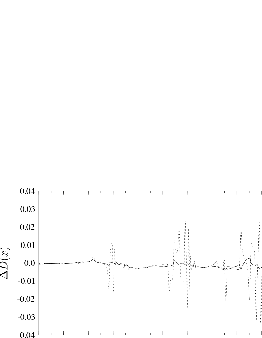
Figure 2: The Fourier cosine transforms $D_{\scriptscriptstyle QM}(x)$ (full) and $D_{\scriptscriptstyle SC}$ (dashed) of the level density, calculated from quantum energies and periodic orbits, respectively.

Figure 3: The differences $D_{\scriptscriptstyle QM}(x)-D_{\scriptscriptstyle SC}(x)$ and $D_{\scriptscriptstyle EBK}(x)-D_{\scriptscriptstyle SC}(x)$ between Fourier cosine transforms of the level density.

Figure 4: The differences $D_{\scriptscriptstyle QM}(x)-D_{\scriptscriptstyle SC}(x)$ between Fourier cosine transforms of the level density with (full) and without (dashed) contributions from interference terms to $D_{\scriptscriptstyle SC}(x)$.

In this section we compare the semiclassical approximation of the last section with exact quantum results. For this purpose we consider a Fourier cosine transform of the oscillatory part of the level density with a Gaussian damping term and a cut-off

$$D(x)=\frac{1}{k_{max}}\int_{0}^{k_{max}}\!\mbox{d}k\,[d(k)-\bar{d}(k)]\,\cos(kx)\,\exp(-z\frac{k^{2}}{k_{max}^{2}})\;.$$ (76)

This function has peaks in the vicinity of the lengths of periodic orbits.

The calculations were carried out for a quarter ellipse with $a=1.1$ and $b=0.9$ and with Dirichlet boundary conditions on all sides. The damping factor was chosen to be $z=5$. The function $D(x)$ was evaluated in three different ways and the results are denoted $D_{\scriptscriptstyle QM}(x)$, $D_{\scriptscriptstyle SC}(x)$ and $D_{\scriptscriptstyle EBK}(x)$. The first function $D_{\scriptscriptstyle QM}(x)$ was obtained from the quantum energies. These energy levels were determined up to energy $E_{max}=20\,000$ by solving the two Mathieu equations (37) and (38) numerically, which corresponds to $1\,198$ energy levels. The second function $D_{\scriptscriptstyle SC}(x)$ was determined by using Eq. (74) with all periodic orbits up to length $l=12$ and $n=30$, and the third function $D_{\scriptscriptstyle EBK}(x)$ was determined from the semiclassical energy levels that are solutions of the EBK-conditions (73).

In figure 2 the results for the quantum spectrum and the trace formula, $D_{\scriptscriptstyle QM}(x)$ and $D_{\scriptscriptstyle SC}(x)$, are compared. Both curves are in good agreement and can hardly be distinguished. For that reason we plot the difference between both curves in figure 3 (dashed line). One can see that the semiclassical error is approximately one order of magnitude smaller than the function $D(x)$. Figure 3 shows also the difference between $D_{\scriptscriptstyle EBK}(x)$ and $D_{\scriptscriptstyle SC}(x)$ (full line) which is much smaller than the difference between $D_{\scriptscriptstyle QM}(x)$ and $D_{\scriptscriptstyle SC}(x)$. This shows that the error which was introduced by deriving the trace formula from the EBK-energies with stationary phase and uniform approximations is much smaller than the original error of the EBK-quantization. This cannot necessarily be expected because the EBK-quantization condition, the trace formula and the stationary phase approximations which connect both approximations are all only valid in leading order of $\hbar$. A similar result was observed previously for a circular billiard with a singular magnetic flux line [41]. The smallness of $D_{\scriptscriptstyle EBK}(x)-D_{\scriptscriptstyle SC}(x)$ shows also that the modifications for contributions of tori near the separatrix due to Eq. (56) are not large in the range where the numerical examination was carried out.

We also show that it is important to include complex orbits, i. e. the interference terms, in (74). In figure 4 the difference $D_{\scriptscriptstyle QM}(x)-D_{\scriptscriptstyle SC}(x)$ is plotted where $D_{\scriptscriptstyle SC}(x)$ was calculated once with (full line) and once without (dashed line) the interference terms. One can see that the semiclassical error is much bigger in the second case, especially near $x=9$. This is due to a torus of complex orbits with $n=5$ and $m=1.5$ which is close to becoming real. It becomes real for $b/a\approx 0.809$ which is near the present value of $b/a=11/9\approx 0.818$.

3 The oval billiard

We discuss now how the semiclassical approximation for the elliptical billiard has to be modified when the ellipse experiences a small perturbation which makes the system non-integrable. We consider in particular a perturbation which consists in a deformation of the ellipse into an oval-shaped billiard system introduced by Berry [30]. It has a parameterization which expresses the radius of curvature $R$ of the boundary as a function of the angle $\Psi$ between the tangent vector and the $x$-direction

$$R(\Psi)=1+\delta\cos(2\Psi)\;,$$ (77)

where $\Psi$ lies in the range $[0,2\pi)$. From this definition the dependence of the $x$- and $y$-coordinates on $\Psi$ follows as [30]

$$x(\Psi) = \sin(\Psi)+\frac{\delta}{2}\sin(\Psi)+\frac{\delta}{6}\sin(3\Psi)$$

$$y(\Psi) = -\cos(\Psi)+\frac{\delta}{2}\cos(\Psi)-\frac{\delta}{6}\cos(3\Psi)\,.$$ (78)

The oval has an area $A=\pi-\pi\delta^{2}/6$, a perimeter $L=2\pi$, two half-axes of lengths $a=1+\delta/3$ and $b=1-\delta/3$, and it is a deformation of an ellipse of order $\delta^{2}$. The billiard can as well be considered as a perturbation of the circle. Then the deformation is of order $\delta$.

Figure 5: Periodic orbits in the oval billiard for $\delta=0.3$. The desymmetrized versions of these orbits in the quarter oval represent all orbits which are reflected up to five times on the oval-shaped boundary.

Numerical examinations were performed for the deformation parameter $\delta=0.3$ for which the half-axes of the oval billiard have the same lengths as those of the elliptical billiard in the last section. We consider again a desymmetrized version of the billiard which consists of a quarter oval with Dirichlet boundary conditions on all sides. For this system the shortest periodic orbits were determined. Figure 5 represents all periodic orbits which are reflected up to five times on the oval-shaped boundary of the quarter oval. We choose to present them by corresponding orbits in the full oval since their structure can be seen more clearly there. All these orbits appear in pairs which are labelled by letters. With the exception of the pair $a$ all pairs of orbits result from the break-up of tori of the ellipse. Since the perturbation is small, no subsequent bifurcations of orbits occur in this length regime.

The differences in the lengths of orbits within a pair are shown in Table 1. With the exception of the first pair the length differences are very small. For that reason, the orbits cannot be treated as isolated orbits in a semiclassical approximation if the energy is not rather high. We discuss in the following the different uniform approximations by which the contributions of the pairs to the semiclassical trace formula can be treated. Most of the pairs ($b,c,d,f,g,i,j,k,l$) result from a break-up of tori of the elliptical billiard with $\alpha>0$, i. e. from tori which have a confocal ellipse as caustic. Their contribution can be treated by the uniform approximation for the generic break-up of tori, that will be described in the next section.

pair	$\bar{l}$	$\Delta l$	$\Delta t$ xl	type
a	2.00000	0.20000	$0.52747$
b	2.83548	0.00705	$0.03875$	e
c	3.00259	0.00051	$0.00265$	e
d	5.23473	0.00249	$0.01208$	e
e	5.43636	0.00025	$-0.00035$	h
f	3.06282	0.00005	$0.00017$	e
g	7.49347	0.00169	$0.02427$	e
h	7.54064	0.00112	$-0.01176$	h
i	3.09101	0.00001	$0.00001$	e
j	5.88609	0.00007	$0.00031$	e
k	8.12883	0.00029	$0.00288$	e
l	9.70973	0.00149	$0.07798$	e
m	9.72132	0.00135	$-0.06491$	h
2b	5.67096	0.01411	$0.61722$	e
3b	8.50644	0.02116	$3.17563$	e

Table 1: Properties of pairs of orbits in the quarter oval. The different columns show the mean length $\bar{l}$ the length difference $\Delta l$ and the quantity $\Delta t=\mbox{Tr\,}M_{1}+\mbox{Tr\,}M_{2}-4$ for a pair of orbits. The type-column specifies whether the pair arose from the break-up of a torus of the ellipse with a confocal ellipse or a confocal hyperbola as caustic, respectively.

Other pairs ($e,h,m$) result from the break-up of tori of the ellipse with $\alpha<0$, i. e. from tori with a confocal hyperbola as caustic. These tori all arose from a bifurcation of the stable orbit in the ellipse, as the eccentricity of the ellipse was increased starting from the circle. These tori are not necessarily well separated from the stable orbit in the ellipse, as is expressed by the interference term in (58), and thus the usual formula for the break-up of tori cannot be used.

The correct contributions of these pairs to the trace formula can be obtained by considering the oval not as a deformation of the ellipse but as a deformation of the circle. Then the pairs ($e,h,m$) are obtained not from the break-up of tori but from bifurcations of the stable orbit along the vertical axis of the billiard (the first orbit of the pair $a$ in figure 5). This stable orbit will be denoted by $a_{s}$ in the following. In particular, the pair $e$ arises from a bifurcation of the 3-fold repetition of the orbit $a_{s}$ at $\delta_{bif}=3/13\approx 0.2308$, the pair $h$ from a bifurcation of the 4-fold repetition of $a_{s}$ at $\delta_{bif}=(39-24\sqrt{2})/41\approx 0.1234$, and the pair $m$ from a bifurcation of the 5-fold repetition of $a_{s}$ at $\delta_{bif}=(63-24\sqrt{5})/121\approx 0.0771$. For the pair $e$ the bifurcation is shown in figure 6 by plotting the orbits for values of $\delta$ near $\delta_{bif}\approx 0.2308$. This bifurcation results in four new orbits in the full oval, the right orbit in figure 6 which can be traversed in both directions and thus represents two orbits, and the left orbit and its mirror image (obtained by reflection on the $y$-axis) which is not plotted.

Figure 6: The period-tripling bifurcation which yields the orbits $e$ of figure 5. The orbits are shown for $\delta=0.230$, $\delta=0.235$ and $\delta=0.240$ (from below), and the bifurcation occurs at $\delta_{bif}=3/13\approx 0.231$.

It follows from the above considerations that the contributions of the pairs $e$, $h$ and $m$ are described by formulas for bifurcations that are discussed in section 3.2. This is a very general property. If one considers an integrable system which depends on an external parameter and in which bifurcations occur that result in the appearance of new tori, then in a slightly perturbed system there are bifurcations which result in a finite number of new orbits. Thus the break-up of tori which are close to a bifurcation is described by formulas for bifurcations in which a finite number of orbits is involved.

3.1 Broken torus contribution

If an integrable system is perturbed then all tori of periodic orbits break up and only a finite number of periodic orbits remain (except for degenerate cases). According to the Poincaré-Birkhoff theorem the number of remaining orbits is even, half them are stable and half of them are unstable. The Poincaré-Birkhoff theorem does not specify the total number of remaining orbits, but generally this number is two [42]. For the semiclassical treatment of this case, i. e. the break-up of a torus into one stable and one unstable orbit, a uniform approximation was derived by Tomsovic, Grinberg and Ullmo [20, 21]. This approximation extends previous results of Ozorio de Almeida [18, 43]. The formula can also be applied to cases in which, due to the presence of discrete symmetries, the break-up of a torus results in $n$ stable and $n$ unstable orbits with respectively identical actions, periods, stabilities and Maslov indices. The uniform approximation for the contributions of these orbits to the level density can be written in the following form

$$d_{bt}(E) = \frac{1}{2\pi\hbar r}\,\sqrt{\frac{2\pi|\Delta S|}{\hbar}}\,\mbox{\bf Re}\,\exp\left\{\frac{i}{\hbar}\bar{S}-\frac{i\pi}{2}\bar{\nu}\right\}$$ (79)

$$\times\left\{\left[\frac{\bar{T}+\frac{\Delta T}{2}}{\sqrt{|\mbox{Tr\,}M_{u}-2|}}+\frac{\bar{T}-\frac{\Delta T}{2}}{\sqrt{|\mbox{Tr\,}M_{s}-2|}}\right]\,\mbox{J}_{0}\left(\frac{\Delta S}{\hbar}\right)\right.$$

$$+\,i\,\left[\frac{T_{u}}{\sqrt{|\mbox{Tr\,}M_{u}-2|}}-\frac{T_{s}}{\sqrt{|\mbox{Tr\,}M_{s}-2|}}\right]\,\mbox{J}_{1}\left(\frac{\Delta S}{\hbar}\right)$$

$$\left.-\phantom{\,i\,}\left[\frac{\frac{\Delta T}{2}}{\sqrt{|\mbox{Tr\,}M_{u}-2|}}-\frac{\frac{\Delta T}{2}}{\sqrt{|\mbox{Tr\,}M_{s}-2|}}\right]\,\mbox{J}_{2}\left(\frac{\Delta S}{\hbar}\right)\right\}\;.$$

In case of the break-up of a torus into $2n$ orbits due to the presence of discrete symmetries the equation has to be multiplied by $n$. The indices $u$ and $s$ correspond to the unstable and stable orbit, respectively. Furthermore

$$\bar{S}=\frac{S_{u}+S_{s}}{2}\;,\;\;\;\Delta S=\frac{S_{u}-S_{s}}{2}\;,\;\;\;\bar{T}=\frac{T_{u}+T_{s}}{2}\;,\;\;\;\Delta T=\frac{T_{u}-T_{s}}{2}\;,\;\;\;\bar{\nu}=\frac{\nu_{u}+\nu_{s}}{2}\;,$$ (80)

and $S$, $T$, $\nu$, $M$ and $r$ denote the action, period, Maslov index, stability matrix and repetition number of an orbit, respectively.

In the following we will use a slightly simplified version of (79) which is obtained by applying the relation $\mbox{J}_{2}(z)=2\,\mbox{J}_{1}(z)/z-\mbox{J}_{0}(z)$. The term $2\,\mbox{J}_{1}(z)/z$ yields a modification of the prefactor of the $\mbox{J}_{1}$-Bessel function which is one order of $\hbar$ smaller than the previous prefactor of $\mbox{J}_{1}$ in (79). Since we consider only the leading order semiclassical approximation we neglect this term and obtain

$$d_{bt}(E)=\frac{1}{\pi\hbar}\,\sqrt{\frac{2\pi|\Delta S|}{\hbar}}\,\left\{\bar{A}\,\mbox{J}_{0}\left(\frac{\Delta S}{\hbar}\right)\,\cos\left(\frac{\bar{S}}{\hbar}-\frac{\pi}{2}\bar{\nu}\right)+\Delta A\,\mbox{J}_{1}\left(\frac{\Delta S}{\hbar}\right)\,\cos\left(\frac{\bar{S}}{\hbar}-\frac{\pi}{2}(\bar{\nu}-1)\right)\right\}\;,$$ (81)

where

$$\bar{A}=\frac{1}{2r}\left[\frac{T_{u}}{\sqrt{|\mbox{Tr\,}M_{u}-2|}}+\frac{T_{s}}{\sqrt{|\mbox{Tr\,}M_{s}-2|}}\right]\;,\;\;\;\Delta A=\frac{1}{2r}\left[\frac{T_{u}}{\sqrt{|\mbox{Tr\,}M_{u}-2|}}-\frac{T_{s}}{\sqrt{|\mbox{Tr\,}M_{s}-2|}}\right]\;.$$ (82)

This approximation, as well as (79), interpolates over the whole regime from the torus contribution to the contributions of isolated periodic orbits in the Gutzwiller approximation. In the limit $\Delta S\rightarrow 0$ the mean amplitude $\bar{A}$ diverges, but the product $\bar{A}\sqrt{|\Delta S|}$ remains finite, and the whole expression yields the Berry-Tabor term for the semiclassical contribution of a torus. In the opposite limit where $\Delta S/\hbar>>1$ one can replace the Bessel functions by their leading order term for large arguments and obtains the Gutzwiller approximation for the contributions of isolated orbits. Finally we note that equation (81) in combination with the definitions (80) and (82) is invariant under exchange of the labels $u$ and $s$. Thus the definitions in (80) and (82) can also be formulated in terms of an orbit 1 and an orbit 2 without specifying which of them is stable and which unstable.

3.2 Contribution of bifurcating orbits

There is only a finite number of generic forms in which periodic orbits in two-dimensional systems bifurcate. They are characterized by normal forms that describe the classical motion in the vicinity of a bifurcation. The different normal forms for generic bifurcations of periodic orbits in two-dimensional systems were derived by Meyer [11] and Bruno [12, 13] and are discussed in [43, 44]. Altogether there are six different kinds of bifurcations which are classified according to the lowest repetition number $m$ of a central orbit for which the bifurcation occurs. (A special case is $m=1$ where there is no orbit before the bifurcation.) There is one kind of bifurcation for $m=1$ up to $m=3$, respectively, two kinds for $m=4$, and one for $m>4$. The corresponding bifurcations are period-$m$-tupling bifurcations, i. e. the primitive periods of the arising periodic orbits are $m$ times the primitive period of the bifurcating central periodic orbit at the bifurcation.

We restrict the discussion in the following to the case $m>4$. This kind of bifurcation is the first that can be observed when an integrable system is perturbed since the higher repetitions of a stable orbit bifurcate earlier than the lower repetitions. It has the following form: a central stable periodic orbit bifurcates and two new periodic orbits appear, one stable and one unstable, while the central orbit remains stable. The new appearing periodic orbits are called satellite orbits.

For the case $m>4$ a uniform approximation was derived in [17] which interpolates over the regime from the bifurcation up to regions where the orbits can be described in the Gutzwiller approximation. This uniform approximation was obtained by an extension of the method of Ozorio de Almeida and Hannay [14].

The final formula in [17] was given for bifurcating periodic orbits in billiard systems and for bifurcating periodic orbits without turning points in systems with potentials. The derivation in [17] can also be applied to orbits with turning points, since only the Maslov index has to be changed. The following uniform formula for the contributions of bifurcating periodic orbits to the level density includes all these cases

$$d_{bif}(E) = \frac{\Theta(\hat{\varepsilon})}{\pi\hbar}\,\sqrt{\frac{2\pi|\Delta S|}{\hbar}}\,\left\{\bar{A}\,\mbox{J}_{0}\left(\frac{\Delta S}{\hbar}\right)\,\cos\left(\frac{\bar{S}}{\hbar}-\frac{\pi}{2}\bar{\nu}\right)+\Delta A\,\mbox{J}_{1}\left(\frac{\Delta S}{\hbar}\right)\,\cos\left(\frac{\bar{S}}{\hbar}-\frac{\pi}{2}(\bar{\nu}-1)\right)\right\}$$ (83)

$$+\mbox{sign}(\hat{\varepsilon})\,\frac{\bar{A}}{\pi\hbar}\,\sqrt{\frac{|\Delta S|}{\hbar}}\,\int_{\Lambda}^{\infty}\!\mbox{d}X\,\frac{\cos\left(\frac{\bar{S}}{\hbar}+\frac{\beta}{2}X^{2}-\frac{\pi}{2}(\nu-\beta)\right)}{X^{2}}+\frac{T_{0}}{\pi\hbar mr}\frac{\cos\left(\frac{S_{0}}{\hbar}-\frac{\pi}{2}\nu_{0}\right)}{\sqrt{|\mbox{Tr\,}M_{0}-2|}}\;.$$

Here $\Lambda=\sqrt{2\beta[S_{0}-\bar{S}]/\hbar}$ and $\hat{\varepsilon}$ is a parameter that is positive when all three orbits are real, and negative when only the central orbit is real. The values of $\nu$ and $\beta$ can be obtained from the Maslov indices of the (real) periodic orbits, since $\nu_{0}=\nu+\mbox{sign}(\hat{\varepsilon})\cdot\beta$, $\nu_{u}=\nu$ and $\nu_{s}=\nu-\beta$. The other quantities are defined in (80) and (82). The repetition number of the central stable orbit is $mr$ where $m$ is the lowest repetition number for which the bifurcation occurs. (When the $m$-th repetition of a periodic orbit bifurcates, then the bifurcation occurs also for all repetition numbers which are a multiple of $m$.) Eq. (83) is valid as long as no subsequent bifurcations of the participating periodic orbits occur before they can be considered isolated. Note that formula (83) in combination with definitions (80) and (82) is again invariant under exchange of the indices $u$ and $s$. The different terms in Eq. (83) can be interpreted in the following way. The first term with the two Bessel functions is a joint contribution of the two satellite orbits. It has a form which is identical to the broken torus contribution (81). The last term in (83) is the semiclassical contribution of the central stable orbit, and the remaining term is an interference term between satellite orbits and central orbit.

The properties of the three orbits that participate in the bifurcation are summarized in Table 2.

	$\hat{\varepsilon}<0:$	$\xi_{0}$ stable,	$\nu_{0}=\nu-1$
	$\hat{\varepsilon}>0:$	$\xi_{0}$ stable,	$\nu_{0}=\nu+1$
$\beta=1$		$\xi_{u}$ unstable,	$\nu_{u}=\nu$
		$\xi_{s}$ stable,	$\nu_{s}=\nu-1$
		$S_{0}>S_{u}>S_{s}$
	$\hat{\varepsilon}<0:$	$\xi_{0}$ stable,	$\nu_{0}=\nu+1$
	$\hat{\varepsilon}>0:$	$\xi_{0}$ stable,	$\nu_{0}=\nu-1$
$\beta=-1$		$\xi_{u}$ unstable,	$\nu_{u}=\nu$
		$\xi_{s}$ stable,	$\nu_{s}=\nu+1$
		$S_{s}>S_{u}>S_{0}$

Table 2: Properties of orbits which participate in a generic period $m$-tupling bifurcation with $m\geq 5$. $\xi_{0}$ denotes the central orbit, and $\xi_{u}$ and $\xi_{s}$ denote the unstable and stable satellite orbits, respectively.

The bifurcations in the oval billiard that lead to the pairs $e$, $h$ and $m$ are not generic. This is due to the symmetries of the billiard system. But the normal forms which describe these bifurcations agree with normal forms of generic bifurcations, namely with those for double the repetition number. For example, the pair $e$ results from a bifurcation of the 3-fold repetition of the orbit $a_{s}$, but its normal form corresponds to that of a generic bifurcation with repetition number $m=6$. This follows from the treatment of bifurcations in the presence of symmetries [45, 46]. It can be understood by considering a Poincaré section of surface perpendicular to the central orbit. For a generic period-$m$-tupling bifurcation with $m>4$, the map from the Poincaré section of surface at some starting point to the Poincaré section of surface after $m$ traversals of the central orbit has $2m$ fixed points near the central orbit (after the bifurcation); $m$ of them correspond to the new stable orbit and $m$ to the new unstable orbit, since both orbits cross the Poincaré section of surface $m$ times before they close. For the considered bifurcations in the oval billiard there are $4m$ instead of $2m$ fixed points in the vicinity of the central orbit, since two new stable and two new unstable orbits arise, but the number and arrangement of stable and unstable fixed points is the same as for a generic period-$(2m)$-tupling bifurcation.

As a consequence, also the period-tripling and period-quadrupling bifurcations of the stable vertical orbit $a_{s}$ in the oval billiard can be described by the formula for generic bifurcations with $m>4$. The only difference is, that $m$ has to be replaced by $2m$ in Eq. (83) and the whole formula has to be multiplied by two, if one considers the bifurcation in the full oval.

In the desymmetrized billiard, the quarter oval, the orbit $a_{s}$ runs along a part of the boundary of the billiard and Eq. (83) has to be modified in a different way. We describe this by first looking at the Gutzwiller contribution of the $n$-th repetition of the orbit $a_{s}$ which is modified to take account of the fact that $a_{s}$ is a boundary orbit

$$\hat{d}_{na_{s}}(E) = \frac{1}{\pi\hbar}\frac{T_{1}}{2n\sqrt{|\mbox{Tr}\,M_{1}-2|}}\cos(\frac{S_{1}}{\hbar}-\frac{\pi}{2}\nu_{1})+\frac{1}{\pi\hbar}\frac{T_{2}}{2n\sqrt{|\mbox{Tr}\,M_{2}-2|}}\cos(\frac{S_{2}}{\hbar}-\frac{\pi}{2}\nu_{2})$$ (84)

$$= \frac{b}{2\pi k}\left[\frac{\sin(2nkb)}{2\sin(nv)}-\frac{\cos(2nkb)}{2\cos(nv)}\right]\,,$$

where $b=1-\delta/3$ and $v=\arcsin(\sqrt{(1-\delta/3)/(1+\delta)})$. The second line in Eq. (84) is given in dimensionless units. The quantities with index 1 are those of the vertical stable orbit in the half oval with Dirichlet boundary conditions on the $x$-axis. Furthermore, $T_{2}=T_{1}$, $S_{2}=S_{1}$, $M_{2}=-M_{1}$ and $\nu_{2}=\nu_{1}+1+2([nv/\pi]\mbox{mod}2)$. Eq. (84) has the form of a sum of contributions from two orbits, each with half the usual amplitude. Bifurcations of the $n$-th repetition of the orbit $a_{s}$ occur when $\delta\neq 0$ and one of the two terms in (84) diverges. The approximation (84) is only valid if the orbit is well separated from a bifurcation. Near a bifurcation it has to be modified by replacing the term which diverges at the bifurcation by Eq. (83) where $m$ is twice the lowest repetition number for which the bifurcation occurs and $r=2n/m$. If both terms are close to a bifurcation then both terms have to be replaced.

In the following we apply the uniform approximation (83) and its modifications in order to describe the break-up of tori of the ellipse with $\alpha<0$. A comparison with the semiclassical contributions of the tori in the elliptical billiard (section 2.3.5) shows that this effectively corresponds to an application of the broken torus approximation (81) to the torus term in Eq. (58). The interference term and the contribution of the bifurcating stable orbit do not change their form. This is related to the fact, that for a generic period-$m$-tupling bifurcation with $m>4$ the differences of the actions of the satellite orbits grow more slowly than the differences between the actions of the satellite orbits and the action of the central stable orbit. This is not the case for all bifurcations. For example, there is a period-doubling bifurcation in the ellipse for a ratio of the half-axis $a/b=\sqrt{2}$. This bifurcation is again described by the approximation Eq. (58) (plus the contribution of the stable orbit), but in this case it is not correct to apply the broken torus approximation (81) to the torus term in Eq. (58) in order to describe the break up of the torus. Instead one has to use the uniform approximation for a generic bifurcation with $m=4$ which has a more complicated form and is described by a diffraction catastrophe integral for the catastrophe $X_{9}$ [14].

3.3 Numerical results

In the following we examine different approximations for the spectral density numerically. For that purpose the energy levels of the quarter oval with $\delta=0.3$ were determined by a boundary element method up to energy $E_{max}=20\,000$. This corresponds to 1190 different energy levels.

In order to compare semiclassical results with quantum mechanical results we consider again the Fourier cosine transform $D(x)$ with a cut-off that is defined in (76). The damping factor is again $z=5$. Figure 7 compares determinations of $D(x)$ from the quantum mechanical spectrum $D_{\scriptscriptstyle QM}(x)$ and the uniform approximation $D_{\scriptscriptstyle CUA}(x)$. For the calculation of $D_{\scriptscriptstyle CUA}(x)$ all periodic orbits up to length $l=12$ and up to 30 reflections on the boundary were included. Both curves are in good agreement and it is difficult to see the differences. For that reason we plot in the following figures the semiclassical error, i. e. the difference between the quantum mechanical curve $D_{\scriptscriptstyle QM}(x)$ and different semiclassical (or uniform) approximations for it.

Figure 7: The Fourier cosine transforms $D_{\scriptscriptstyle QM}(x)$ (full) and $D_{\scriptscriptstyle CUA}$ (dashed) of the level density, calculated from quantum energies and periodic orbits, respectively.

Figure 8: The semiclassical errors $D_{\scriptscriptstyle QM}(x)-D_{\scriptscriptstyle QT}(x)$ (dotted) and $D_{\scriptscriptstyle QM}(x)-D_{\scriptscriptstyle QTI}(x)$ (full) for the quasi-torus approximation with and without interference terms, respectively.

The most basic semiclassical approximation for a quasi-integrable system, i. e. for a slightly perturbed integrable system, is the quasi-torus approximation. In this approximation the pairs of periodic orbits are treated as if they still contribute like a torus of periodic orbits. We use here a quasi-torus approximation in which the semiclassical amplitudes and phases are determined directly from the corresponding periodic orbits. This is done by setting $\Delta S$ equal to zero in Eq. (81). This approximation is used for all pairs of orbits except for the pair $a$ and its repetitions. For this pair the action difference is already quite large, and the orbits are treated as separate periodic orbits. In more detail, the contribution of the $n$-th repetition of the unstable orbit $a_{u}$ is approximated by

$$\hat{d}_{na_{u}}(E)=\frac{a(-1)^{n}}{2\pi k}\left[\frac{\cos(2nka-n\frac{\pi}{2})}{2\sinh(nu)}-\frac{\cos(2nka-n\frac{\pi}{2})}{2\cosh(nu)}\right]\,,$$ (85)

with $a=1+\delta/3$ and $u=\mbox{arccosh}(\sqrt{(1+\delta/3)/(1-\delta)})$, and the contributions of the stable orbit $a_{s}$ and its repetitions by Eq. (84).

The semiclassical error for the quasi-torus approximation $D_{\scriptscriptstyle QM}(x)-D_{\scriptscriptstyle QT}(x)$ is plotted as dotted line in figure 8. This approximation already works relatively good. This is due to the fact that the action differences within pairs of orbits are still relatively small and that the orbits are not very close to a bifurcation. However, in comparison with the semiclassical error for the ellipse in figure 3 the semiclassical error for the quasi-torus approximation in figure 8 is clearly larger. The scales of the plots differ by approximately 50%. In order to improve the approximation we apply Eq. (83) for the pairs of orbits which arose from a bifurcation, i. e. for the pairs $e$, $h$ and $m$, but we still set the action differences in formulas (81) and (83) equal to zero. Note that with this substitution Eq. (83) has exactly the same form as that of the contribution of a torus near a bifurcation (see section 2.3.5). This approximation can thus be considered as an improved quasi-torus approximation which takes into account cases in which quasi-tori are close to a bifurcation. The corresponding semiclassical error $D_{\scriptscriptstyle QM}(x)-D_{\scriptscriptstyle QTI}(x)$ is plotted in figure 8 as full line. One can see an clear improvement near $x\approx 5.4$. This length corresponds to the pair $e$ which is that pair out of $e$, $h$ and $m$ which is closest to a bifurcation. This can be seen from the differences between the mean lengths of the pairs and the $m$-th repetition of the central orbit from which they arose by a bifurcation: $\bar{l}_{e}-3l_{a_{s}}=0.03636$, $\bar{l}_{h}-4l_{a_{s}}=0.34064$, and $\bar{l}_{m}-5l_{a_{s}}=0.72132$. The pairs $h$ and $m$ are already well separated from the orbit $a_{s}$ and thus the inclusion of the interference term does not improve the approximation.

For a further improvement of the semiclassical approximation we apply now the uniform approximations (81) and (83) without setting $\Delta S$ equal to zero. The result $D_{\scriptscriptstyle QM}(x)-D_{\scriptscriptstyle UA}(x)$ is shown in figure 9 as full line. For a comparison with the previous approximation the function $D_{\scriptscriptstyle QM}(x)-D_{\scriptscriptstyle QTI}(x)$ is plotted again as dotted line. One can observe a clear improvement of the approximation at three places which correspond to the first three repetitions of the pair $b$. Table 1 shows that this is the pair for which the length difference is largest, and the size of the semiclassical error increases with the size of $\Delta l$. We note that for the decrease of the semiclassical error it is important to use the whole formula (81) and not only the first term with the $\mbox{J}_{0}$-Bessel function. A criterion for the importance of the second term is the size of $\Delta t$ in Table 1 which increases rapidly with the repetition number of the pair $b$.

Figure 9: The semiclassical errors $D_{\scriptscriptstyle QM}(x)-D_{\scriptscriptstyle QTI}(x)$ (dotted) and $D_{\scriptscriptstyle QM}(x)-D_{\scriptscriptstyle UA}(x)$ (full) for the quasi-torus approximation with interference term and for the uniform approximation, respectively.

Figure 10: The semiclassical errors $D_{\scriptscriptstyle QM}(x)-D_{\scriptscriptstyle UA}(x)$ (dotted) and $D_{\scriptscriptstyle QM}(x)-D_{\scriptscriptstyle CUA}(x)$ (full) for the uniform approximation with and without the contribution of a pair of complex orbits, respectively.

Even for the uniform approximation there is still a relatively large error at $x\approx 9$. This error is due to the fact that up to now we considered only contributions from real orbits to the spectral density. But before a bifurcation there are also contributions from complex orbits as is expressed by the interference term in Eq. (83). The error at $x\approx 9$ is due to fact that the 5-fold repetition of the orbit $a_{s}$ is close to a second bifurcation which occurs at $\delta_{bif}=(75-24\sqrt{5})/61\approx 0.3497$. In a last step we improve the approximation by taking into account the contribution of these complex orbits. This is done by determining these orbits for values $\delta>\delta_{bif}$ where they are real. From these data the properties of the orbits can be extrapolated into the complex region. The final result $D_{\scriptscriptstyle QM}(x)-D_{\scriptscriptstyle CUA}(x)$ is shown in figure 10 as full line. For a comparison with the previous approximation the function $D_{\scriptscriptstyle QM}(x)-D_{\scriptscriptstyle UA}(x)$ is plotted again as dotted line. As one can see, the error is clearly decreased near $x=9$ by including the contribution of the complex orbits, and the final semiclassical error is of the same size as in the elliptical billiard. This shows that by using the uniform approximations (81) and (83) the same accuracy of the semiclassical approximation can be achieved as in the unperturbed integrable system.

4 Conclusions

Most applications of semiclassical trace formulas in the literature have concentrated on cases where the periodic orbits are either isolated or occur in families. These approximation are valid only in restricted classes of systems. In general systems, it is common that semiclassical contributions of periodic orbits cannot be considered isolated from contributions of other periodic orbits in their neighbourhood. This requires the use of uniform approximations which take account of the underlying classical structures and yield joint contributions of neighbouring periodic orbits. In systems where the classical phase space has regular and chaotic regions this is a generic situation, and semiclassical quantization rules in terms of periodic orbits in these systems always involve uniform approximations. But uniform approximations can also be necessary in integrable or chaotic systems, for example when bifurcations of periodic orbits occur in integrable systems or when periodic orbits are close to creeping or diffractive orbits in chaotic billiard systems [47, 48].

In the first part of this paper we examined an integrable system, a billiard in form of an ellipse, and derived a trace formula for it. The elliptical billiard is a standard example for an integrable system, yet its semiclassical trace formula is more complicated than a summation over semiclassical contributions of isolated tori. These complications are due to the presence of the separatrix and of the stable periodic orbit. We were particularly interested in the treatment of the bifurcations of the stable orbit and its connection to generic bifurcations when the ellipse is perturbed. We derived a semiclassical trace formula which takes account of these bifurcations, and we examined its semiclassical accuracy.

In the second part of this paper we deformed the ellipse into an oval which is non-integrable. It was shown that in the quasi-integrable regime it is not always sufficient to treat the break-up of tori by the general formulas of [18, 20, 21]. If a torus in the integrable system is close to a bifurcation, then uniform formulas for general bifurcations are needed for describing its break-up. In the numerical section it was shown that with the uniform formulas for the break-up of tori and for the bifurcations the same semiclassical accuracy can be achieved as in the unperturbed integrable system.

If the billiard system is deformed more, then the stable periodic orbits of the billiard undergo further bifurcations. A semiclassical description of a system in the truly mixed regime, i. e. not in the near-integrable regime, requires the use of uniform approximations for all generic bifurcations [49]. In case that the system has discrete symmetries there are further bifurcations which are specific for the considered symmetry. The application of uniform approximations for these bifurcations requires not only the determination of all real periodic orbits up to some length, but also of all complex periodic orbits which are close to becoming real. Additional complications can arise when a periodic orbit undergoes several subsequent bifurcations which cannot be considered isolated. This shows, as is well-known, that semiclassical trace formulas for systems with mixed phase space are definitely more complicated as for integrable or chaotic systems.

Acknowledgments

I am obliged to E. Bogomolny for many helpful suggestions and discussions. It is a pleasure to thank also O. Bohigas, M. Brack and H. R. Dullin for fruitful discussions, and, furthermore, H. R. Dullin for communicating results of [37] before publication. This work was supported by the Alexander von Humboldt-Stiftung and by the Deutsche Forschungsgemeinschaft under contract No. DFG-Ste 241/7-1 and /6-1.

References

- [1] P. Cvitanović (Ed.). Periodic orbit theory – theme issue. CHAOS, 2:1–158, 1992.
- [2] T. Tél and E. Ott (Eds.). Chaotic scattering – theme issue. CHAOS, 3:417–782, 1993.
- [3] G. Casati and B. Chirikov (Eds.). Quantum Chaos. Cambridge University Press, Cambridge, 1995.
- [4] M. C. Gutzwiller. Periodic orbits and classical quantization conditions. J. Math. Phys., 12:343–358, 1971.
- [5] R. Balian and C. Bloch. Distribution of eigenfrequencies for the wave equation in a finite domain: III. Eigenfrequency density oscillations. Ann. Phys., 69:76–160, 1972.
- [6] M. V. Berry and M. Tabor. Closed orbits and the regular bound spectrum. Proc. R. Soc. Lond. A., 349:101–123, 1976.
- [7] M. V. Berry and M. Tabor. Calculating the bound spectrum by path summation in action-angle variables. J. Phys. A: Math. Gen., 10:371–379, 1977.
- [8] M. C. Gutzwiller. Chaos in Classical and Quantum Mechanics. Springer, New York, 1990.
- [9] S. C. Creagh and R. G. Littlejohn. Semiclassical trace formulas in the presence of continuous symmetries. Phys. Rev. A, 44:836–850, 1991.
- [10] S. C. Creagh and R. G. Littlejohn. Semiclassical trace formulae for systems with non-Abelian symmetry. J. Phys. A, 25:1643–1669, 1992.
- [11] K. R. Meyer. Generic bifurcations of periodic points. Trans. Am. Math. Soc., 149:95–107, 1970.
- [12] A. D. Brjuno. Instability in a Hamiltonian system and the distribution of asteroids. Math. USSR Sbornik, 12:271–312, 1970.
- [13] A. D. Bruno. Research on the restricted three body problem. I: Periodic solutions of a Hamiltonian system. Preprint No. 18, Moskva: Inst. Prikl. Mat. Akad. Nauk SSSR. 44p. (Russian), 1972.
- [14] A. M. Ozorio de Almeida and J. H. Hannay. Resonant periodic orbits and the semiclassical energy spectrum. J. Phys. A: Math. Gen., 20:5873–5883, 1987.
- [15] M. Kuś, F. Haake, and D. Delande. Prebifurcation periodic ghost orbits in semiclassical quantization. Phys. Rev. Lett., 71:2167–2171, 1993.
- [16] K. M. Atkins and G. S. Ezra. Semiclassical density of states at symmetric pitchfork bifurcations in coupled quartic oscillators. Phys. Rev. A, 50:93–97, 1994.
- [17] M. Sieber. Uniform approximation for bifurcations of periodic orbits with high repetition numbers. J. Phys. A, 29:4715–4732, 1996.
- [18] A. M. Ozorio de Almeida. Semiclassical energy spectrum of quasi-integrable systems. In T. Seligman, editor, Quantum Chaos and Statistical Nuclear Physics (Lecture Notes in Physics 263), pages 197–211. Springer, New York, 1986.
- [19] S. C. Creagh. Trace formula for broken symmetry. Ann. Phys., 248:60–94, 1996.
- [20] S. Tomsovic, M. Grinberg, and D. Ullmo. Semiclassical trace formulas of near-integrable systems: Resonances. Phys. Rev. Lett., 75:4346–4349, 1995.
- [21] D. Ullmo, M. Grinberg, and S. Tomsovic. Near-integrable systems: Resonances and semiclassical trace formulas. Phys. Rev. E, 54:136–152, 1996.
- [22] P. J. Richens. On quantisation using periodic classical orbits. J. Phys. A: Math. Gen., 15:2101–2110, 1982.
- [23] Y. Ayant and R. Arvieu. Semiclassical study of particle motion in two-dimensional and three-dimensional elliptical boxes: I. J. Phys. A, 20:397–409, 1987.
- [24] R. Arvieu and Y. Ayant. Semiclassical study of particle motion in two-dimensional and three-dimensional elliptical boxes: II. J. Phys. A, 20:1115–1136, 1987.
- [25] I. S. Gradshteyn and I. M. Ryzhik. Table of Integrals, Series, and Products. Academic Press, San Diego, 1980. Corrected and enlarged edition.
- [26] J. B. Keller and S. I. Rubinow. Asymptotic solution of eigenvalue problems. Ann. Phys., 9:24–75, 1960. Errata in Ann. Phys., 10:303–305, 1960.
- [27] Ya. G. Sinai. Introduction to Ergodic Theory. Princeton University Press, Princeton, NJ, 1976.
- [28] S.-J. Chang and R. Friedberg. Elliptical billiards and Poncelet’s theorem. J. Math. Phys., 29:1537–1550, 1988.
- [29] B. Crespi, S.-J. Chang, and K.-J. Shi. Elliptical billiards and hyperelliptic functions. J. Math. Phys., 34:2257–2289, 1993.
- [30] M. V. Berry. Regularity and chaos in classical mechanics, illustrated by three deformations of a circular ’billiard’. Eur. J. Phys., 2:91–102, 1981.
- [31] M. B. Tabanov. Billiard in an ellipse, geodesics on an ellipsoid, and new elliptic coordinates. Russian Acad. Sci. Dokl. Math., 48:438–444, 1994.
- [32] S. Okai, H. Nishioka, and M. Ohta. Periodic orbits in elliptic billiards. Mem. Konan Univ., Sci. Ser., 37:29–45, 1990.
- [33] P. H. Richter, A. Wittek, M. P. Kharlamov, and A. P. Kharlamov. Action integrals for ellipsoidal billiards. Z. Naturforsch., 50a:693–710, 1995.
- [34] P. M. Morse and H. Feshbach. Methods of Theoretical Physics, Part I and II. McGraw - Hill, New York, 1953.
- [35] M. Abramowitz and I. A. Segun, editors. Handbook of Mathematical Functions. Dover, New York, 1965.
- [36] A. J. S. Traiber, A. J. Fendrik, and M. Bernath. Level crossings and commuting observables for the quantum elliptic billiard. J. Phys. A, 22:L365–L370, 1989.
- [37] H. R. Dullin, H. Waalkens, and J. Wiersig. In preparation.
- [38] I. Ussishkin. The quantization of billiards in the scattering approach beyond the semiclassical approximation. M. Sc. Thesis, Weizmann Institute of Science, 1994.
- [39] G. Tanner. How chaotic is the stadium billiard: A semiclassical analysis. Preprint: chao-dyn/9610013, 1996.
- [40] E. B. Bogomolny. Smoothed wave functions of chaotic quantum systems. Physica D, 31:169–189, 1988.
- [41] S. M. Reimann, M. Brack, A. G. Magner, J. Blaschke, and M. V. N. Murthy. Circular quantum billiard with a singular magnetic flux line. Phys. Rev. A, 53:39–48, 1996.
- [42] A. J. Lichtenberg and M. A. Lieberman. Regular and Chaotic Dynamics. Springer, New York, 1992. Second edition.
- [43] A. M. Ozorio de Almeida. Hamiltonian Systems: Chaos and Quantization. Cambridge University Press, Cambridge, 1988.
- [44] V. I. Arnold (Ed.). Dynamical Systems III. Mathematical Aspects of Classical and Celestial Mechanics. Springer, Berlin, 1993.
- [45] R. J. Rimmer. Generic Bifurcations for Involutory Area Preserving Maps. Memoirs of the AMS No. 272. American Mathematical Society, Providence, Rhode Island, 1982.
- [46] M. A. M. De Aguiar, C. P. Malta, M. Baranger, and K. T. R. Davies. Bifurcations of periodic trajectories in non-integrable Hamiltonian systems with two degrees of freedom: Numerical and analytical results. Ann. Phys., 180:167–205, 1987.
- [47] H. Primack, H. Schanz, U. Smilansky, and I. Ussishkin. Penumbra diffraction in the quantization of dispersing billiards. Phys. Rev. Lett., 76:1615–1618, 1996.
- [48] M. Sieber, N. Pavloff, and C. Schmit. Uniform approximation for diffractive contributions to the trace formula in billiard systems. Submitted to Phys. Rev. E, 1996.
- [49] H. Schomerus and M. Sieber. In preparation.