Intermittency and the Slow Approach
to Kolmogorov Scaling

Abstract

From a simple path integral involving a variable volatility in the velocity differences, we obtain velocity probability density functions with exponential tails, resembling those observed in fully developed turbulence. The model yields realistic scaling exponents and structure functions satisfying extended self-similarity. But there is an additional small scale dependence for quantities in the inertial range, which is linked to a slow approach to Kolmogorov (1941) scaling occurring in the large distance limit.

The universal features displayed by fully developed hydrodynamic turbulence are still not fully understood. Kolmogorov (1941) [1, 2] showed how a set of statistical quantities known as structure functions are expected depend on the length scale $r$ as power laws with predicted exponents. Experimental measurements have indicated that while these predictions are close to the truth, the predicted exponents are not exactly realized. In the face of this experimental input, much effort has been devoted towards understanding the origin of these anomalies in the scaling exponents, while retaining the notion that current experiments are observing an “inertial range” where strict power law scaling holds.

In this paper we will investigate what appears to be a loop-hole in this reasoning. In spite of impressive advances made in the experimental studies, the fact remains that the scaling exponents have been deduced by looking at scaling regions extending over little more than one decade in $r$ [3, 4, 5, 6]. This leaves open the possibility that a small but significant departure from strict power law scaling is still consistent with the data. We will argue that this possible departure is sufficient to allow the observed anomalies in the exponents to be nothing more than a transient effect related to intermittency, and that the true power law scaling only occurs on larger scales. This very large distance scaling could take the form proposed by Kolmogorov.

We shall present a model which predicts deviations from power law scaling, and which shows that these deviations may be small enough to have escaped detection thus far. The model is based on a simple physical picture for the effects of intermittency, which are effects due to the coming and going of coherent structures in the velocity field. We will model the effects that these structures (eddies) have directly on the probability distribution function (PDF) for velocity differences. We are claiming simplicity in our approach, but not uniqueness. Thus the applicability to 3-dimensional hydrodynamical turbulence in particular could be considered speculative, since the model makes no mathematical contact with the Navier-Stokes equations. On the other hand, when the consequences of the model are explicitly worked out they are found to coincide rather well with the data.

Only the symmetric part of the observed PDF will be modeled in this paper. This is denoted by $P_{r}(\delta v_{r})$ where $\delta v_{r}$ is the difference in some velocity component at two points separated by a distance $r$. The model will yield an explicit expression for the PDF which 1) for small $r$ has the typical sharp peak and broad tails characteristic of intermittent behavior, 2) at any finite $r$ displays exponential tails at large enough $\delta v_{r}$, and 3) tends toward a Gaussian form in the large $r$ limit. But the model shows that these realistic features may in fact be implying that the values of the scaling exponents are slightly scale dependent, as they evolve from their observed “anomalous” values for the values of $r$ where they are presently measured, to the pure K41 values in the large $r$ limit.

We consider a discrete set of points on the line connecting the two points separated by distance $r$. We label the points by their distance from one end, $(0,r_{1},r_{2},...,r_{N},r_{N+1})$ where $r_{N+1}=r$. We start by assuming that $P_{r}(\delta v_{r})$ can be approximated by

$$P_{N}(v_{r}-v_{0})=\left[{\prod\limits_{l=1}^{N}\int_{-\infty}^{\infty}dv_{r_{l}}}\right]{\cal P}(v_{r}-v_{r_{N}}){\cal P}(v_{r_{N}}-v_{r_{N-1}})\cdots{\cal P}(v_{r_{1}}-v_{0}),$$ (1)

with $\int_{-\infty}^{\infty}{\cal P}(y)dy=1$. We assume that the set of points $r_{j}$ is characterized by a scale $\rho$ such that $({r}_{j}/\rho)^{a}=j$, where $j=1,2,...,N+1$ and $a$ is a positive constant to be determined below. The integration over all velocities at the intermediate points may be thought of as a sum over all paths in the space of velocities which start at $v_{0}$ and end at $v_{r}$. We could thus refer to (1) as a path integral. But note that we refrain from taking the continuum limit, $N\rightarrow\infty$ with $r$ fixed, since the scale $\rho$ has a physical significance.

The discretization of the range from 0 to $r$ into subregions $(r_{j},r_{j+1})$ is associated with our modeling of intermittent behavior. Roughly speaking, we are suggesting that the coming and going of eddies, of sizes comparable to subregion size $r_{j+1}-r_{j}$, produce a variable volatility in the typical velocity differences $v_{r_{j+1}}-v_{r_{j}}$. We make this statement precise by writing ${\cal P}(v_{r_{j}}-v_{r_{j-1}})$ as a superposition of Gaussians, where we integrate over all values of a volatility parameter $s_{j}$ which is itself weighted according to a Gaussian. To simplify notation we denote $v_{r_{j}}=x_{j}$.

$${\cal P}(x_{j}-x_{j-1}) = \int_{-\infty}^{\infty}P_{\rm Gauss}(s_{j}\sigma,x_{j}-x_{j-1}){\rm exp}(-s_{j}^{2}){\frac{ds_{j}}{\sqrt{2\pi}}}$$ (2)

$$P_{\rm Gauss}(\sigma,x) = {\frac{1}{\sqrt{2\pi}\sigma}}{\rm exp}\left({-{\frac{x^{2}}{2\sigma^{2}}}}\right)$$ (3)

The consideration of large and small values of $s_{j}$ corresponds to the possible presence or absence of eddies in that subregion at various times. Note that the variance of both ${\cal P}(x_{j}-x_{j-1})$ and $P_{\rm Gauss}(\sigma,x)$ is $\sigma^{2}$.

(1) is constructed to give the cumulative effect of the variable volatilities occurring in the various subregions. $\rho$ should be typical of scales on which viscosity influences and damps the formation of eddies. As such $\rho$ is expected to lie between the dissipative (Kolmogorov) scale, $\eta$, and the lower end of the inertial scaling range (the latter range being characterized by the absence of viscosity effects). Note that if $0<a<1$ then the size of the subregion, $r_{j+1}-r_{j}$, and thus the relevant eddy size for that subregion, would increase with $j$.

We proceed by inserting (2) into (1) and integrating over the $x_{j}$. We can write the terms in the exponential which depend on $y\equiv(x_{1},x_{2},...,x_{N})$ in matrix notation $y^{T}My+Jy$ where $M$ is a matrix and $J$ is a vector, with the latter depending on $x_{0}$ and $x_{N+1}$. We may complete the square and do the Gaussian integrations over $y$, for various values of $N$. From this we are able to deduce a simple result, where all dependence on the $s_{j}$ now resides in $\hat{S}^{2}\equiv\sum_{j=1}^{N+1}s_{j}^{2}$. The $s_{j}$ integrations for fixed $\hat{S}$ then just give the surface area of an $N+1$ dimensional sphere.

$$P_{N}(x_{N+1}-x_{0})$$ (4)

$$= {\frac{1}{\sigma(2\pi)^{{\frac{N}{2}}+1}}}\left[{\prod\limits_{j=1}^{N+1}\int_{-\infty}^{\infty}ds_{j}}\right]{\frac{1}{\hat{S}}}{\rm exp}\left({-{\frac{(x_{N+1}-x_{0})^{2}}{2\sigma^{2}\hat{S}^{2}}}-{\frac{1}{2}}\hat{S}^{2}}\right)$$

$$= {\frac{1}{\sigma(2\pi)^{{\frac{N}{2}}+1}}}\left({{\frac{2\pi^{{\frac{N+1}{2}}}}{\Gamma({\frac{N+1}{2}})}}}\right)\times\int_{0}^{\infty}d\hat{S}\hat{S}^{N-1}{\rm exp}\left({-{\frac{(x_{N+1}-x_{0})^{2}}{2\sigma^{2}\hat{S}^{2}}}-{\frac{1}{2}}\hat{S}^{2}}\right)$$

$$= {\frac{\left({(N+1)/2}\right)^{{\frac{N}{2}}}}{\sigma\sqrt{\pi}\Gamma({\frac{N+1}{2}})}}\int_{0}^{\infty}dSS^{N-1}{\rm exp}\left({-{\frac{(x_{N+1}-x_{0})^{2}}{2\sigma^{2}S^{2}(N+1)}}-{\frac{1}{2}}S^{2}(N+1)}\right)$$

In the last step we have defined $S^{2}\equiv\hat{S}^{2}/(N+1)$ for convenience.

Finally we will take this result and analytically continue from integer values $N+1$ to positive real values $\tau$. Replacing $N+1$ by $\tau\equiv(r/\rho)^{a}$ gives

$$P_{r}(\delta v_{r})={\frac{\left({\tau/2}\right)^{{\frac{\tau-1}{2}}}}{\sigma\sqrt{\pi}\Gamma(\tau/2)}}\int_{0}^{\infty}dSS^{\tau-2}{\rm exp}\left({-{\frac{(\delta v_{r})^{2}}{2\sigma^{2}S^{2}\tau}}-{\frac{1}{2}}S^{2}\tau}\right).$$ (5)

We note that for large $\tau$ the integral over $S$ becomes strongly peaked about $S=1$, and thus

$$P_{r}(\delta v_{r})\stackrel{{\scriptstyle\tau\rightarrow\infty}}{{\rightarrow}}{\frac{1}{\sigma\sqrt{2\pi\tau}}}{\rm exp}\left({-{\frac{(\delta v_{r})^{2}}{2\sigma^{2}\tau}}}\right).$$ (6)

In addition we find, for any $\tau$, that the variance in the velocity differences is

$$\left\langle{(\delta v_{r})^{2}}\right\rangle=\sigma^{2}\tau=\sigma^{2}(r/\rho)^{a}.$$ (7)

The variable $\tau$ controls the evolution of the PDF, in the sense that evolution through unit steps in $\tau$ are generated by successive application of the “evolution operator” in (2). In this sense $\tau$ is an “evolutionary” time scale depending on the distance scale $r$. There is also a dynamical time scale associated with scale $r$, the eddy turnover time, which is simply $r/v$ where $v$ is a typical velocity observed on scale $r$. If we associate $v$ with $\sigma\sqrt{\tau}$ from (7), and if the evolutionary and dynamical times happen to scale with $r$ in the same way, then we obtain $a=2/3$. This gives the standard scaling law $\left\langle{(\delta v_{r})^{2}}\right\rangle\propto r^{2/3}$.

We now perform the integral over $S$, and rescale the PDF such that the variance is unity for all $\tau$. We obtain

$$\hat{P}_{\tau}(x)={\frac{\tau^{({\frac{1}{4}}(1+\tau))}}{\sqrt{\pi}2^{{\frac{1}{2}}(\tau-1)}\Gamma({\frac{1}{2}}\tau)}}{\left|{x}\right|}^{{\frac{1}{2}}(\tau-1)}K_{{\frac{1}{2}}(\tau-1)}(\left|{x}\right|\tau^{1/2}).$$ (8)

$K_{\nu}(y)$ is the modified Bessel function of the second kind. In Fig. (1) we display $\hat{P}_{\tau}(x)$ for various $\tau$.

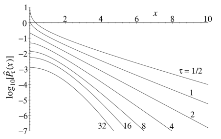
Figure 1: $\log_{10}[\hat{P}_{\tau}(x)]$ vs. $x$ for $\tau=1/2,1,2,4,8,16,32$, top to bottom. The curves are vertically displaced by $0.5,0,-0.5,-1,-1.5,-2,-2.5$ respectively.

When $\tau$ is an even integer, $\hat{P}_{\tau}(x)$ is an exponential times a polynomial in $x$, and in particular for $\tau=2$ it is purely exponential, $\hat{P}_{2}(x)={\rm exp}(-\left|{x}\right|\sqrt{2})/\sqrt{2}$. For $\tau<2$ the PDF is even more strongly peaked and it decreases less quickly than an exponential (“stretched exponential”), before becoming purely exponential at large enough $x$. For $\tau>2$ we have “deformed Gaussians” with exponential tails. For any $\tau$, $d{\rm ln}\hat{P}_{\tau}(x)/dx\stackrel{{\scriptstyle x\rightarrow\infty}}{{\rightarrow}}-\sqrt{\tau}$. Alternatively we may consider moments, $M_{\tau}^{n}\equiv\int\hat{P}_{\tau}(x)\left|{x}\right|^{n}dx$, which are all finite and given by

$$M_{\tau}^{n}={\frac{2^{n}}{\sqrt{\pi\tau^{n}}}}{\frac{\Gamma({\frac{n+1}{2}})\Gamma({\frac{n+\tau}{2}})}{\Gamma({\frac{\tau}{2}})}}.$$ (9)

The approach to the exponential tails is reflected in $M_{\tau}^{n+1}/((n+1)M_{\tau}^{n})\stackrel{{\scriptstyle n\rightarrow\infty}}{{\rightarrow}}1/\sqrt{\tau}$.

It is common to describe the evolution of the PDF with $r$ in terms of the generalized structure functions, defined by $S_{n}(r)=\left\langle{\left|{\delta v_{r}}\right|^{n}}\right\rangle$. For $r$ in the inertial range it is usually assumed that $S_{n}(r)\propto r^{\zeta_{n}}$. Our model suggests that exactly scale independent exponents do not exist for the typical ranges of $r$ considered, and that instead we should consider the local exponents $\zeta_{n}(r)\equiv d\log(S_{n}(r))/d\log(r)$. We obtain

$$\zeta_{n}(r)={\frac{a}{2}}\tau\left({\Psi({\frac{1}{2}}(n+\tau))-\Psi({\frac{1}{2}}\tau)}\right),$$ (10)

where $\Psi$ is the digamma function. This gives $\zeta_{2}(r)=a$, and in the large $r$ limit, $\zeta_{n}(\infty)=an/2$. The latter is K41 scaling when $a=2/3$. Although we adopt this value of $a$ in the following, we leave open the question of whether $a$ is exactly equal to $2/3$ or just close to it. We also stress that we are describing only the symmetric part of the observed PDF, which in the case of the PDF for longitudinal velocity differences also has an asymmetric part. This asymmetry is reflected by the nonvanishing of the structure functions $\left\langle{\delta v_{\parallel r}^{n}}\right\rangle$ for odd $n$. In particular our $\zeta_{3}$ is not the same as the scaling exponent of $\left\langle{\delta v_{\parallel r}^{3}}\right\rangle$, which is constrained to be unity [2, 8].

In Fig. (2) we display $\zeta_{n}(r)$ for various $r$, and compare to the large $r$ limit values $\zeta_{n}=n/3$.

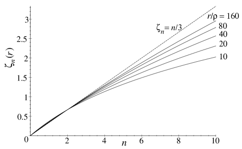
Figure 2: $\zeta_{n}(r)$ vs. $n$ for $r/\rho=10,20,40,80,160$, bottom to top. The dashed line is $\zeta_{n}=n/3$.

The main point is that the scaling exponents approach their asymptotic values very slowly. It is also of interest that for some range of $r/\rho$, our exponents are realistic for a wide range of $n$. We show this by comparing to the model of She and Leveque (SL)[9], which yields $\zeta^{SL}_{n}=n/9+2-2\left({2/3}\right)^{n/3}$, and which is known to fit the current data quite well. We may phrase the agreement in terms of the relative scaling exponents $\zeta_{n}/\zeta_{3}$, which are known to better accuracy [3, 4, 5, 6] than the individual exponents, and for which the factor $a$ in (10) cancels. We find, for example, that $\zeta_{n}(35\rho)/\zeta_{3}(35\rho)$ as a function of $n$ is within a few percent of the corresponding SL values up to $n=30$! And as $r$ varies from 20 to 50, $\zeta_{6}(r)/\zeta_{3}(r)$ for example varies from 1.72 to 1.82, compared to $\zeta^{SL}_{6}/\zeta^{SL}_{3}=1.78$.

To see the $r$ dependence of the structure functions themselves we display $S_{n}(r)$ in Fig. (3).

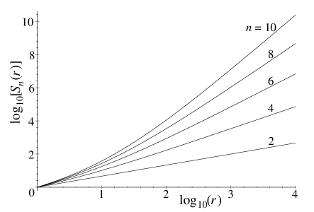
Figure 3: $\log_{10}[S_{n}(r)]$ vs. $\log_{10}(r)$ with $\rho=1$ for $n=2,4,6,8,10$, bottom to top, each line vertically offset so as to vanish at $r=1$.

Over some range of $r$ the lines appear to be close to straight. But other than for $n=2$, which is exactly straight, the lines have a positive curvature which increases for larger $n$. We will see below how these positive curvatures, or equivalently the scale dependence of the scaling exponents, may be rather subtle to observe experimentally. But first we must consider the effects of viscosity on the structure functions.

We expect that the effects of viscosity will cause $\tau=(r/\rho)^{2/3}$ to be replaced by a function $f(r)$ which deviates from $(r/\rho)^{2/3}$ as $r$ approaches the dissipative scale $\eta$ from above. Since a decreasing $\tau$ corresponds to increasing intermittency, and since the cause of intermittency in our picture—variable volatility of velocity differences—should be damped by viscous effects, we expect that $f(r)$ should start to decrease more slowly than $(r/\rho)^{2/3}$. Thus the evolution of the PDF shapes is retarded by viscous effects in the “intermediate viscous range”, the range of $r$ between $\eta$ and the start of the inertial range. The implication is that at large scales in the inertial range where $f(r)=(r/\rho)^{2/3}$ it is likely that $\rho>\eta$. We may also expect that $\rho/\eta$ grows with the size of the intermediate viscous range.

For very small $r$ where the velocity field is smooth the variance is evolving like $r^{2}$, faster than in the inertial range, and thus there must clearly be a decoupling between the evolution of the PDF shapes and the evolution of the PDF variance. We are thus led to a generalization of our model, where we replace the expression in (5) by the following.

$$P_{r}(\delta v_{r})={\frac{\left({f(r)/2}\right)^{(f(r)-1)/2}}{\sqrt{\pi g(r)/f(r)}\Gamma(f(r)/2)}}\int_{0}^{\infty}dSS^{f(r)-2}{\rm exp}\left({-{\frac{(\delta v_{r})^{2}}{2S^{2}g(r)}}-{\frac{1}{2}}S^{2}f(r)}\right)$$ (11)

This new PDF has the property that $\left\langle{(\delta v_{r})^{2}}\right\rangle=g(r)$, and thus we can use $g(r)$ to reproduce the observed behavior of the variance even in regions where viscosity or finite size effects are important. The function $f(r)$ determines the evolution of the PDF shapes; that is, the new $\hat{P}_{r}(x)$ is obtained from the one in (8) by replacing $\tau$ with $f(r)$.

We will illustrate the effects of viscosity with specific choices for $f(r)$ and $g(r)$. We consider $f(r)=\left({[r+\rho-\eta]/\rho}\right)^{2/3}$, which is unity at $r=\eta$ and approaches $(r/\rho)^{2/3}$ at large $r$. For $g(r)$ in the range $\eta<r<10^{4}\eta$ we consider

$$g(r)=\left[{c_{1}-c_{2}e^{[1-{\frac{r}{\eta}}]/c_{4}}-c_{3}e^{[1-10^{4}{\frac{\eta}{r}}]/c_{5}}}\right](r/\eta)^{2/3}.$$

We take two examples for $(c_{1},c_{2},c_{3},c_{4},c_{5})$ which idealize typical data sets, $g_{1}(r)$ with $(80,79,60,10,5)$ having a relatively large inertial range (large Reynolds number) and $g_{2}(r)$ with $(80,79,70,5,30)$ having a small inertial range. Our results are not very sensitive to precisely how these functions deviate from $r^{2/3}$ behavior outside the inertial range. Note that the intermediate viscous range is larger for $g_{1}(r)$. Due to our expectation that $\rho$ should increase with the size of the intermediate viscous range it is natural that $\rho_{1}>\rho_{2}$. For illustrative purposes only, we choose $\rho_{1}=4.3\eta$ and $\rho_{2}=1.3\eta$.

With this input we can extract all higher order structure functions from (11). The scaling in the inertial range for both cases turns out (because of our fortuitous choice of $\rho_{1}$ and $\rho_{2}$) to be described by the realistic scaling exponents $\zeta_{n}(35\rho)$ from (10). We show this in Fig. (4) where we plot $S_{n}(r)/r^{\zeta_{n}(35\rho)}$.

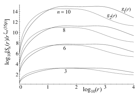
Figure 4: $\log_{10}[S_{n}(r)/r^{\zeta_{n}(35\rho)}]$ vs. $\log_{10}(r)$ with $\eta=1$ for $n=3,6,8,10$, bottom to top. The solid and dashed lines correspond to $g_{1}(r)$ and $g_{2}(r)$ respectively.

Of most interest are the $n=8,10$ curves for the $g_{1}(r)$ case, where we see (very slight!) evidence of a double hump structure growing more prominent with increasing $n$. This positive curvature in the middle of the scaling region is arising from the positive curvatures in Fig. (3), which in turn is a reflection of the gradual approach to K41 scaling. This is the generic signature of our model, which should be seen when the size of the inertial range and the order $n$ are both large enough. The figure makes it clear, though, that it is a small effect which may be hidden in present data.

Our model may also be used to illustrate “extended self-similarity” [10, 6]. In Fig. (5) we plot $S_{n}(r)$ versus $S_{3}(r)$ for $4<r/\eta<10^{4}$ for the two cases $g_{1}(r)$ and $g_{2}(r)$.

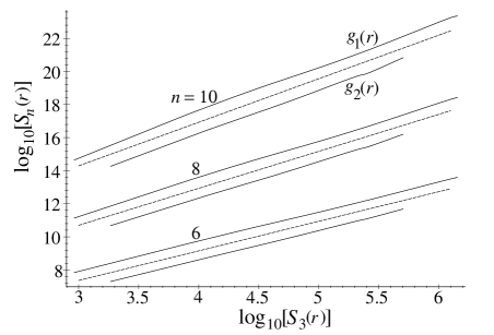
Figure 5: $\log_{10}[S_{n}(r)]$ vs. $\log_{10}[S_{3}(r)]$ for $4<r/\eta<10^{4}$ and for $n=6,8,10$, bottom to top. The lines for the $g_{1}(r)$ and $g_{2}(r)$ cases are displaced by 0.5 and $-0.5$ respectively. The dashed straight lines have slopes $\zeta_{n}(35\rho)/\zeta_{3}(35\rho)$.

For comparison we add straight lines with slopes given by the relative exponents $\zeta_{n}(35\rho)/\zeta_{3}(35\rho)$. We see that scaling has been extended to smaller scales than is apparent in Fig. (4). Similar results are obtained for other choices of the functions $f(r)$ and $g(r)$. It thus appears that such plots are not very sensitive to the deviations from power law scaling we are proposing.

We reiterate that the model yields a universal set of local scaling exponents, and the scaling exponent from an experiment depends on what distance scale, effectively, the local scaling exponent is being measured at relative to $\rho$. On the other hand if it is true that $\rho/\eta$ increases with the size of the intermediate viscous region, as we are suggesting, then it may be difficult to obtain measurements at distances, in units of $\rho$, which are very different from each other. The variability in the scaling exponents is also obscured if different experiments have intermediate viscous regions of similar size, and/or if one is confined to the lower order structure functions, such as $n=6$ and below.

We have seen how viscosity and finite size effects can have the effect of transforming the structure functions in Fig. (3) into the structure functions in Fig. (4) which in turn display extended self-similarity in Fig. (5). It is also encouraging to find that realistic values of the scaling exponents emerge when the $\rho$ parameter is within the intermediate viscous range. But perhaps most important is that the model suggests how evidence for a slow approach to K41 scaling could eventually be uncovered. We should also differentiate between the evolution of the PDF shapes as a function of $r$ (to which the structure functions are sensitive), and the basic set of shapes predicted by the model, given in (8) and depicted in Fig. (1). These probability density functions may be of interest in various other contexts.

References

- [1] A. N. Kolmogorov, Dokl. Akad. Nauk SSSR 30, 9 (1941).
- [2] U. Frisch, “Turbulence: The Legacy of A.N. Kolmogorov”, Cambridge University Press (1995).
- [3] A. Arneodo, et. al., Europhy. Lett. 34, 411 (1996).
- [4] J. Herweijer and W. van de Water, Phys. Rev. Lett. 74, 4651 (1995).
- [5] P. Tabeling, G. Zocci, F. Belin, J. Maurer, and H. Willaime, Phys. Rev. E53, 1613 (1995); F. Belin, P. Tabeling, H. Willaime, Physica D93, 52 (1996).
- [6] R. Benzi, S. Ciliberto, C. Baudet, G. R. Chavarria, Physica D80, 385 (1995); R. Benzi, L. Biferale, S. Ciliberto, M.V. Strugila and T. Tripiccione, Physica D96, 162 (1996).
- [7] B. Castaing, Y. Gagne, and E. Hopfinger, Physica D46, 177 (1990).
- [8] A. N. Kolmogorov, Dokl. Akad. Nauk SSSR 32, 16 (1941).
- [9] Z.-S. She and E. Leveque, Phys. Rev. Lett. 72, 336 (1994).
- [10] R. Benzi, S. Ciliberto, R. Tripiccione, C. Baudet, E. Massaioli and S. Succi, Phys. Rev. E48, 29 (1993).