Mixed Quantum-Classical versus Full Quantum Dynamics: Coupled Quasiparticle-Oscillator System

Abstract

The relation between the dynamical properties of a coupled quasiparticle-oscillator system in the mixed quantum-classical and fully quantized descriptions is investigated. The system is considered to serve as a model system for applying a stepwise quantization. Features of the nonlinear dynamics of the mixed description such as the presence of a separatrix structure or regular and chaotic motion are shown to be reflected in the evolution of the quantum state vector of the fully quantized system. In particular it is demonstrated how wave packets propagate along the separatrix structure of the mixed description and that chaotic dynamics leads to a strongly entangled quantum state vector. Special emphasis is given to view the system from a dynamical Born-Oppenheimer approximation defining integrable reference oscillators and elucidating the role of the nonadiabatic couplings which complements this approximation into a rigorous quantization scheme.

I Introduction

The relation between the quantum and classical dynamics of nonlinear systems includes a specific side in the correspondence between the dynamical properties of systems treated in the mixed and fully quantized descriptions. Various aspects of the correspondences between classical nonlinear systems on the one side and their fully quantized counterparts on the other have been intensively investigated in the last decade (see e. g. [1, 2, 3]). In many systems relevant for molecular and condensed matter physics the direct quantization of the full system in one step is, however, not possible from a practical point of view. As a rule such systems divide naturally into interacting subsystems. Then a stepwise quantization is applied resulting in a mixed description, in which one of the subsystems is treated in the quantum and the other in the classical context. Furthermore in complex systems the mixed description is often necessary for understanding global dynamical properties, e. g. the presence of bifurcations and separatrix structures dividing the solution manifold into characteristic parts, before for a selected energy region the full quantization can be performed.

This stepwise quantization is the basic idea on which the Born - Oppenheimer approximation developed in the early days of quantum mechanics for the quantization of systems dividing into subsystems is based. As is well known this approximation can be complemented into a rigorous scheme, if the nonadiabatic couplings are included [4]. These couplings can be the source of nonintegrability and chaos of systems treated in the mixed quantum-classical description [5, 6]. Then the problem of the quantum-classical correspondences arises on the level of the relation between the dynamical properties of the mixed and fully quantized descriptions [6].

In this paper we consider this dynamic relation for the particular model of a quasiparticle moving between two sites and coupled to oscillators. This is an important model system with applications such as excitons moving in molecular aggregates and coupled to vibrations, see e. g.  [7]. It has also attracted widespread attention in the context of the spin-boson Hamiltonian and its classical-quantum phase space behavior and correspondence (see e. g. [8, 9, 10] and references therein). Hence it seems appropriate to use this system as a model to analyze the relation between the mixed and fully quantized descriptions. Treating the oscillators in the classical or quantum contexts, whereas the quasiparticle moving between two sites is a quantum object from the beginning, one arrives at mixed and fully quantized levels of description. We have recently investigated the dynamical properties of this model in the mixed description by integrating the corresponding Bloch-oscillator equations and demonstrated the presence of a phase space with an underlying separatrix structure for overcritical coupling and chaos developing from the region of the hyperbolic point at the center of this structure. For increasing total energy chaos spreads over the product phase space of the system constituted by the Bloch sphere and oscillator plane, leaving only regular islands in the region of the antibonding states [11]. Here we consider the problem of the relation between the dynamics in the mixed and fully quantum levels of description of the coupled quasiparticle-oscillator motion. Investigating this relation we focus on the adiabatic parameter range, where the closest correspondence between the classical and quantum aspects of the oscillator dynamics can be expected. Although several aspects of the dynamics of the system have been considered [8, 10], there exists no systematic investigation in the adiabatic parameter range. In particular, such an investigation requires the numerical determination of a large number of eigenstates for the fully quantized system. The stationary properties of these states were reported in [12]. In this paper these states are used to compute the dynamics of the fully quantized system and to compare the quantum evolution with the dynamics of the mixed description where the oscillator is treated classically. Performing this comparison we use both the fixed and adiabatic basis sets in the mixed description. The latter basis set is of particular importance to clarify the role of the nonadiabatic couplings in the formation of the dynamics. We demonstrate the effect of the separatrix structure of the mixed description in the oscillator wave packet propagation of the fully quantized version, of dynamical subsystem correlations deriving from the separatrix structure and how the chaotic phase space regions of the system in the mixed description show up in the nonstationary properties of the time dependent full quantum state vector.

In section II the model will be specified in detail. The mixed quantum-classical description is discussed in section III including the derivation of the equations of motion, the fixed point structure and the dynamical properties of the system on this level of description. In section IV the evolution of the fully quantized system is presented and compared to the dynamics in the mixed description.

II The Model

We consider a quasiparticle coupled to oscillator degrees of freedom. The quasiparticle is specified as a molecular exciton in a tight binding representation and can be substituted by any other quantum object moving between discrete sites and described by a tight binding Hamiltonian of the same structure. The system has the Hamiltonian

$$H^{{\rm(tot)}}=H^{{\rm(exc)}}+H^{{\rm(vib)}}+H^{{\rm(int)}},$$ (1)

where $H^{{\rm(exc)}}$, $H^{{\rm(vib)}}$ and $H^{{\rm(int)}}$ are the excitonic, vibronic and interaction parts, respectively. $H^{{\rm(exc)}}$ represents the quantum subsystem, which is taken in the site representation

$$H^{{\rm(exc)}}=\sum_{n}\epsilon_{n}|c_{n}|^{2}+\sum_{n\neq m}V_{nm}c_{n}^{*}\,c_{m},$$ (2)

where $c_{n}$ is the quantum probability amplitude of the exciton to occupy the $n$-th molecule and $V_{nm}$ the transfer matrix element. For the intramolecular vibrations coupling to the exciton we use the harmonic approximation in $H^{{\rm(vib)}}$

$$H^{{\rm(vib)}}={1\over 2}\sum_{n}(p_{n}^{2}+\omega_{n}^{2}q_{n}^{2}).$$ (3)

Here $q_{n}$, $p_{n}$ and $\omega_{n}$ are the coordinate, the canonic conjugate momentum and frequency of the intramolecular vibration of the $n$-th molecule, respectively. The interaction Hamiltonian $H^{{\rm(int)}}$ represents the dependence of the exciton energy on the intramolecular configuration for which we use the first order expansion in $q_{n}$

$$H^{{\rm(int)}}=\sum_{n}\gamma_{n}q_{n}|c_{n}|^{2},$$ (4)

where $\gamma_{n}$ are the coupling constants. The interaction is restricted to a single oscillator at each molecule. The case of a symmetric two site system $n=1,2$, e. g.  an exciton in a molecular dimer constituted by two identical monomers, is considered in what follows. For this case we set $\epsilon_{1}=\epsilon_{2}$, $\omega_{1}=\omega_{2}$, $\gamma_{1}=\gamma_{2}$ and $V_{12}=V_{21}=-V$, $V>0$. Then by introducing for the vibronic subsystem the new coordinates and momenta

$$q_{\pm}:={q_{2}\pm q_{1}\over\sqrt{2}}\hskip 28.45274ptp_{\pm}:={p_{2}\pm p_{1}\over\sqrt{2}},$$ (5)

and for the excitonic subsystem the Bloch variables

$$x=\rho_{21}+\rho_{12},\hskip 28.45274pty=i(\rho_{21}-\rho_{12}),\hskip 28.45274ptz=\rho_{22}-\rho_{11},$$ (6)

where $\rho_{mn}$ is the density matrix of the excitonic subsystem

$$\rho_{mn}=c_{n}^{*}c_{m},$$ (7)

the relevant part of (1)-(4) connected with the exciton coupled to the $q_{-}$ vibration is obtained in the form

$$H_{-}=-Vx+{1\over 2}(p_{-}^{2}+\omega^{2}q_{-}^{2})+{\gamma q_{-}z\over\sqrt{2}}\,.$$ (8)

The part corresponding to $q_{+}$ is not coupled to the exciton and omitted.

The Hamiltonian (8) can be represented as an operator in the space of the two dimensional vectors $C=(c_{1},c_{2})$ constituted by the excitonic amplitudes $c_{n}$ by using the standard Pauli spin matrices $\sigma_{i}$ $(i=x,y,z)$. Passing in (8) to dimensionless variables by measuring $H$ in units of $2V$ and replacing $q_{-}$, $p_{-}$ by

$$Q:=\sqrt{2V}q_{-}\hskip 28.45274ptP:={1\over\sqrt{2V}}p_{-},$$ (9)

one finally obtains

$$H=-{\sigma_{x}\over 2}+{1\over 2}(P^{2}+r^{2}Q^{2})+\sqrt{p\over 2}r\,Q\sigma_{z}\,.$$ (10)

Here

$$p={\gamma^{2}\over 2V\omega^{2}}$$ (11)

represents the dimensionless excitonic-vibronic coupling and

$$r={\omega\over 2V}$$ (12)

is the adiabatic parameter measuring the relative strength of quantum effects in both subsystems. We focus on the adiabatic case $r\ll 1$ when the vibronic subsystem can be described in the classical approximation. To make contact with the dynamical features following from the adiabatic approximation we derive the basic equations in both the fixed and the adiabatic bases.

III Mixed Quantum-Classical Description

A Fixed Basis

In this case the basis states are given by the fixed molecule sites $|n\rangle$ . Representing the excitonic state by $|\psi\rangle=\sum_{n}c_{n}|n\rangle$, inserting it into the time dependent Schroedinger equation for (10) and using (6) the quantum equations of motion for the excitonic subsystem describing the transfer dynamics between the two sites are obtained. The classical equations for the dynamics of the oscillator are found by passing to the expectation values of $Q$ and $P$ and using (10) as a classical Hamiltonian function from which the canonical equations are derived. In this way one obtains the coupled Bloch-oscillator equations representing the dynamics of the system in the mixed description

$$\dot{x} = -\sqrt{2p}\,r\,Q\,y$$ (13)

$$\dot{y} = \sqrt{2p}\,r\,Q\,x+z$$ (14)

$$\dot{z} = -y$$ (15)

$$\dot{Q} = P$$ (16)

$$\dot{P} = -\,r^{2}Q-\sqrt{p\over 2}\,rz$$ (17)

Besides the energy

$$E=-{x\over 2}+{1\over 2}(P^{2}+r^{2}Q^{2})+\sqrt{p\over 2}rQz$$ (18)

there is a second integral of the motion restricting the flow associated with the quantum subsystem to the surface of the unit radius Bloch sphere

$$R^{2}=x^{2}+y^{2}+z^{2}=1\,.$$ (19)

Sometimes it is advantageous to make use of this conserved quantity in order to reduce the number of variables to four, e. g. when a formulation in canonically conjugate variables is desired also for the excitonic subsystem. One then introduces an angle $\phi$ by

$$x=\sqrt{1-z^{2}}\cos\phi\,,\hskip 28.45274pty=\sqrt{1-z^{2}}\sin\phi\,.$$ (20)

We shall replace the usual Bloch variables by these coordinates where it is appropriate.

B Adiabatic Basis

In this case one first solves the eigenvalue problem of the part of the Hamiltonian (10) which contains excitonic operators

$$h^{{\rm(ad)}}=-{\sigma_{x}\over 2}+\sqrt{p\over 2}rQ\sigma_{z}\,,$$ (21)

where $Q$ is considered as an adiabatic variable. The eigenvalues of (21) are given by

$$\epsilon_{\pm}^{{\rm(ad)}}(Q)\,=\pm{1\over 2}w(Q),$$ (22)

where

$$w(Q)\,=\sqrt{1+2pr^{2}Q^{2}}.$$ (23)

The eigenvalues are part of the adiabatic potentials for the slow subsystem

$$U_{\pm}^{{\rm(ad)}}(Q)={1\over 2}r^{2}Q^{2}+\epsilon_{\pm}^{{\rm(ad)}}(Q)\,,$$ (24)

The two eigenstates $(\alpha=1,2)$ of (21) represented by the fixed basis are given by

$$|\alpha=2,Q\rangle={1\over\sqrt{2}}(-\sqrt{1+c(Q)}\,|2\rangle+\sqrt{1-c(Q)}\,|1\rangle)$$ (25)

and

$$|\alpha=1,Q\rangle={1\over\sqrt{2}}(+\sqrt{1-c(Q)}\,|2\rangle+\sqrt{1+c(Q)}\,|1\rangle)$$ (26)

with

$$c(Q):={\sqrt{2p}rQ\over w(Q)}\,.$$ (27)

The state vector of the excitonic subsystem is expanded in the adiabatic basis $|\psi\rangle=\sum_{\alpha}c^{{\rm(ad)}}_{\alpha}|\alpha,Q\rangle$ and inserted into the time dependent Schrödinger equation. For obtaining the complete evolution equations in the adiabatic basis one has to take into account the time derivative of the expansion coefficients $c^{{\rm(ad)}}_{\alpha}$ as well as the nonadiabatic couplings due to the time dependence of the states $|\alpha,Q(t)\rangle$. The neglect of these couplings would result in the adiabatic approximation. Using $(d/dt)|\alpha,Q\rangle=\dot{Q}(d/dQ)|\alpha,Q\rangle$ the nonadiabatic coupling function

$$\varphi_{\alpha\beta}:=\left\langle\alpha,Q\left|{\partial\over\partial Q}\right|\beta,Q\right\rangle,$$ (28)

$(\varphi_{\alpha\beta}=-\varphi_{\beta\alpha})$ is found, which in case of the eigenstates (25,26) is explicitly given by

$$\varphi_{12}=-\frac{\sqrt{p}r}{\sqrt{2}[w(Q)]^{2}}\,.$$ (29)

Introducing now analogously to (6) the Bloch variables in the adiabatic basis and treating the oscillator in the classical approximation one obtains the coupled Bloch-oscillator equations in the adiabatic basis

$$\dot{x}^{{\rm(ad)}} = 2P\,\varphi_{12}(Q)\,z^{{\rm(ad)}}-w(Q)\,y^{{\rm(ad)}}$$ (30)

$$\dot{y}^{{\rm(ad)}} = w(Q)\,x^{{\rm(ad)}}$$ (31)

$$\dot{z}^{{\rm(ad)}} = -2P\,\varphi_{12}(Q)\,x^{{\rm(ad)}}$$ (32)

$$\dot{Q} = P$$ (33)

$$\dot{P} = -r^{2}Q+\sqrt{p}\,w(Q)\varphi_{12}\,x^{{\rm(ad)}}-\sqrt{p\over 2}\,r\,c(Q)\,z^{{\rm(ad)}}$$ (34)

The energy is now expressed by the adiabatic Bloch variable $z^{{\rm(ad)}}$

$$E=w(Q){z^{{\rm(ad)}}\over 2}+{1\over 2}\left(P^{2}+r^{2}Q^{2}\right)$$ (35)

and the flow is again located on the surface of the unit Bloch sphere. Neglecting the nonadiabatic couplings $\varphi_{12}=0$ one obtains the dynamics of the decoupled adiabatic oscillators. The adiabatic oscillators can be considered as one dimensional integrable subsystems corresponding to the Hamiltonians

$$h_{\pm}^{{\rm(ad)}}={1\over 2}P^{2}+U_{\pm}^{{\rm(ad)}}(Q)\,,$$ (36)

where $U_{\pm}^{{\rm(ad)}}(Q)$ is given by (24). The connection between the Bloch variables in the fixed and the adiabatic basis is given by
$x=-c(Q)x^{{\rm(ad)}}-\sqrt{1-c(Q)^{2}}\,z^{{\rm(ad)}}\hskip 28.45274pt$ $x^{{\rm(ad)}}=-c(Q)x-\sqrt{1-c(Q)^{2}}\,z$ $y=-y^{{\rm(ad)}}$ $y^{{\rm(ad)}}=-y$ $z=c(Q)z^{{\rm(ad)}}-\sqrt{1-c(Q)^{2}}x^{{\rm(ad)}}$ $z^{{\rm(ad)}}=c(Q)z-\sqrt{1-c(Q)^{2}}x$

$$\sqrt{1-z^{2}}\,\sin\phi=-\sqrt{1-(z^{{\rm(ad)}})^{2}}\,\sin\phi^{{\rm(ad)}}$$ (37)

Using these transformation formulas one can show that the equations of motion (13) derived in the fixed basis are actually equivalent to those in the adiabatic basis (30).

C Fixed points and bifurcation

Essential information about the phase space of the excitonic-vibronic coupled dimer is contained in the location and the stability properties of the fixed points of the mixed quantum-classical dynamics. Setting in the equations of motion for the fixed basis (13) all time derivatives to zero, we find for any stationary state

$$Q_{s}=-{1\over r}\sqrt{p\over 2}z_{s}\,,\hskip 28.45274ptP_{s}=0\,,\hskip 28.45274pty_{s}=0$$

$$z_{s}-px_{s}z_{s}=0\,.$$ (38)

The stability properties of a fixed point are determined by a linearization of the equations of motion using canonical variables [11].

It is appropriate to subdivide all stationary points according to whether they are located in the bonding region $x_{s}>0$ or in the antibonding region $x_{s}<0$. There is no transition between these two groups when the parameters of the system are varied since $x_{s}=0$ is excluded by (38). This terminology is in accordance with molecular physics where it is common to refer to the state $x=1$ with symmetric site occupation amplitudes $c_{1}=c_{2}$ as bonding and to the state $x=-1$ with antisymmetric amplitudes $c_{1}=-c_{2}$ as antibonding.

1 Bonding region ($x_{s}>0$)

We consider the bonding region first. The location of the fixed points is obtained from (38) using the additional restriction

$$x_{s}^{2}+z_{s}^{2}=1\,.$$ (39)

One finds the following solutions in dependence on the value of the dimensionless coupling strength $p$:

  

(A) $0\leq p\leq 1$: In this case (38) allows for a single solution only.

$${\bf g:}\hskip 28.45274ptx_{s}=1\,,\hskip 28.45274ptz_{s}=0\,,\hskip 28.45274ptQ_{s}=0\,,\hskip 28.45274ptE_{s}=-{1\over 2}$$ (40)

This point is the bonding ground state corresponding to a symmetric combination of the excitonic amplitudes $c_{1}=c_{2}=1/\sqrt{2}$. $\bf g$ is stable elliptic.

  

(B) $p\geq 1$: A bifurcation has occurred and we obtain three stationary points.

$$\begin{array}[]{ccc}{\bf g_{\pm}:}&x_{s}={1\over p}&z_{s}=\pm{\sqrt{p^{2}-1}\over p}\\ &Q_{s}=\pm{\sqrt{p^{2}-1}\over\sqrt{2p\,}r}&E_{s}=-{p^{2}+1\over 4p}\end{array}$$ (41)

These two points are stable elliptic.

$${\bf h:}\hskip 28.45274ptx_{s}=1\,,\hskip 28.45274ptz_{s}=0\,,\hskip 28.45274ptQ_{s}=0\,,\hskip 28.45274ptE_{s}=-{1\over 2}$$ (42)

The point $\bf h$ is at the position of the former ground state, but in contrast to $\bf g$ it is unstable hyperbolic.

The parameter $p$ governs a pitchfork bifurcation: The ground state g below the bifurcation ($p<1$) splits into two degenerate ground states $\bf g_{\pm}$ above bifurcation ($p>1$). At the former ground state a hyperbolic point $\bf h$ appears. This situation is also obvious from fig. 1(a).

2 Antibonding region ($x_{s}<0$)

Independent on the coupling strength $p$ we have in this region only one solution of (38) (see fig. 1(b)):

$${\bf e:}z_{s}=0\,,\hskip 28.45274ptx_{s}=-1\,,\hskip 28.45274ptQ_{s}=0\,,\hskip 28.45274ptE_{s}=+{1\over 2}$$ (43)

This stationary state corresponds to an antisymmetric combination of the excitonic amplitudes $c_{1}=-c_{2}=1/\sqrt{2}$. $\bf e$ is stable for

$$\frac{|r^{2}-1|}{r}>2\sqrt{p}\,,$$ (44)

which holds when the system is not in resonance and in particular for the adiabatic case $r\ll 1$.

Since the equations of motion in the fixed and in the adiabatic basis are equivalent, it is clear that the fixed same points (38) can also be obtained from (30). Setting in (30) the time derivatives of $x$, $y$ and $Q$ equal to zero, one finds for the stationary states of the adiabatic case

$$x_{s}^{{\rm(ad)}}=0\,,\hskip 28.45274pty_{s}^{{\rm(ad)}}=0\,,\hskip 28.45274ptP_{s}^{{\rm(ad)}}=0\,,$$ (45)

leaving for the stationary values of $z_{s}^{{\rm(ad)}}$ the poles

$$z_{s}^{{\rm(ad)}}=\pm 1$$ (46)

It is worth noting that in the adiabatic basis the stationary states are always located at $z^{{\rm(ad)}}_{s}=\pm 1$ and this will be the case for any system treated in mixed quantum-classical description and restricted to the two lowest adiabatic levels. A specific feature of using the adiabatic basis is the independence of the location of the fixed points on the explicit form of the nonadiabatic coupling function since this function enters the equations of motion in form of the products $\varphi_{12}(Q)P$ and $\varphi_{12}(Q)x^{{\rm(ad)}}$ which drop out at a fixed point because of (45) and (46). From (37) it is moreover easy to see that the fixed points in the bonding region are located within the lower adiabatic potential while the antibonding fixed points belong to the upper one. The eq. $\dot{P}=0$ reduces to

$$(w(Q)+pz_{s}^{{\rm(ad)}})Q=0\,.$$ (47)

For $z^{{\rm(ad)}}_{s}=+1$ the only solution of (47) is $Q_{s}=0$, whereas for $z^{{\rm(ad)}}_{s}=-1$ one obtains additional solutions for $p>1$. These solutions are easily seen to correspond to the bifurcation discussed above.

D Integrable Approximations

Before we investigate the dynamics of the complete coupled equations of motion (13) or (30) we would like to mention two integrable approximations to the model. The first and trivial integrable approximation is to set in the equations of motion in the fixed basis (13) $p=0$ which results in a decoupling of the excitonic and vibronic motions. The second and more interesting integrable approximation is obtained by neglecting the nonadiabatic coupling function $\varphi_{12}=0$ in the equations of motion (30) of the adiabatic basis which defines the adiabatic approximation from a dynamical point of view. In this approximation some of the nonlinear features of the model are still contained in the integrable adiabatic reference oscillators (36). In particular the lower adiabatic potential (24) displays the bifurcation from a single minimum structure to the characteristic double well structure when the parameter $p$ (11) passes through the bifurcation value $p=1$. It is also important to note that the fixed point structure is not changed when the nonadiabatic couplings are switched off: Neglecting $\varphi_{12}$ in (30) results in the same fixed points equations as in the case including the nonadiabatic couplings. From the formal side the neglect of $\varphi_{12}$ not necessarily leads to $z_{s}^{{\rm(ad)}}=\pm 1$: According to the equations of motion(30) $\varphi_{12}=0$ implies $z_{s}^{{\rm(ad)}}=const$. Then in the dynamics of the adiabatic approximation both adiabatic modes can be occupied and only the transitions between them are switched off. The oscillator equations become autonomous describing regular motions according to the classical Hamilton function (35) with $z_{s}^{{\rm(ad)}}$ as a parameter. The oscillator coordinate $Q(t)$ enters the Bloch equations for $x(t)$ and $y(t)$. The equations for the latter describe the regular motion on a circle generated by an intersection of the Bloch sphere with the plane $z_{s}^{{\rm(ad)}}=const$ on which the phase oscillations between the modes are realized.

In the following we demonstrate that the regular structures associated with the adiabatic approximation are present in both the mixed and fully quantized descriptions. At the same time we show that the complete coupled system of Bloch-oscillator equations, i. e. including the nonadiabatic couplings, displays dynamical chaos. This identifies the nonadiabatic couplings as a source of nonintegrability and chaos in the mixed description of the system and rises the question about the signatures of this chaos after full quantization is performed. The latter problem will be addressed in the last section.

E Dynamical Properties

The dynamical properties of the coupled Bloch-oscillator equations (13) were analyzed by a direct numerical integration. Some of our results, such as the presence of chaos in the mixed description of the excitonic-vibronic coupled dimer, were reported in [11]. Therefore the aim of this section is twofold: On the one side we reconsider the findings in [11] relating the dynamical structures to the adiabatic approximation, in which the integrable reference systems (36) can be defined. This clarifies the role of the nonadiabatic couplings in the formation of the dynamics of the model, which was not done before. On the other side we provide the necessary characterization of the phase space structure, such as the location of the separatrix dividing the phase space into trapped and detrapped solutions, and the identification of the regions and associated parameters belonging to the regular and chaotic parts of the dynamics, respectively. The latter points will provide the basis to perform the comparison of the mixed description with the full quantum evolution in the next section.

The numerical integration of the equations of motion in the mixed description can be performed both in the fixed (13) and the adiabatic basis (30). The integration in the fixed basis, however, is numerically simpler and the fixed Bloch variables provide a more convenient frame for the excitonic motion. Hence we used the fixed basis for a numerical integration. It must be stressed, however, that the representation of the excitonic system in the fixed and the adiabatic basis are equivalent, if the nonadiabatic couplings are included. The connection between both representations is given by the eqs. (37).

In view of the existence of two integrals of the motion three variables from the total of five variables of the system are independent. Therefore a standard two dimensional Poincaré surface of section is defined by fixing one variable. According to the choice of variables sections can be defined for both the oscillatory and excitonic subsystems. The dynamics of the system was found to depend crucially on the choice of the total energy with respect to the characteristic energies of the system such as the minima of the adiabatic potentials and above the bifurcation the energy corresponding to the hyperbolic fixed point $E_{h}$. Above the bifurcation the separatrix structure, which divides the phase space into characteristic parts, is present. The regular phase space structure following from the integrable adiabatic reference oscillators (36) above the bifurcation is shown in fig. 1.

In fig. 2(a) a Poincaré section in oscillator variables is presented for the value $p=0.8$ which is below the bifurcation value $p=1$. In this case the adiabatic potential $U_{-}(Q)$ has a single minimum. The total energy is chosen at $E=0$, i.ẽ. well below the minimum of the upper adiabatic potential. Therefore the influence of this potential is small and the oscillator dynamics can be expected to be close to the regular dynamics of the lower reference oscillator associated with $U_{-}(Q)$. This is indeed confirmed by fig. 2(a). There is, however, a chain of small resonance islands in the outer part of the section, which is due to resonance between the oscillator motion and the occupation oscillations between the adiabatic modes corresponding to the finite $\dot{z}^{{\rm(ad)}}$ in the case of the presence of the nonadiabatic couplings. The interaction between the occupation oscillations due to the finite $\dot{z}^{{\rm(ad)}}$ and the oscillator motion becomes much more pronounced for higher energies. A corresponding Poincaré section is displayed in fig. 2(b) for the same value $p=0.8$ of the coupling constant, but with the energy now chosen above the minimum of the upper adiabatic potential. This choice of the energy allows according to (35) for a much broader range for the variation of the variable $z^{{\rm(ad)}}$ and consequently the nonadiabatic couplings are more effective. Correspondingly we observe now several resonance chains.

Increasing the coupling above the bifurcation value $p=1$, but fixing the total energy below $E_{h}$ one expects regular oscillations around the displaced minima of the double well structure in $U_{-}(Q)$. A Poincaré section in the oscillator variables corresponding to this behavior is shown in fig. 3(a), where $p=3.4$ and the total energy is below the saddle point of the potential $U_{-}(Q)$. Increasing the energy to a value slightly above $E_{h}$ one finds sections displaying oscillations resembling the separatrix structure as shown in fig. 3(b).

For energies well above $E_{h}$ chaotic trajectories do exist. Characteristic examples are provided by the Poincaré sections in oscillator variables displayed in fig. 3(c) and (d), where the regions of regular and chaotic behavior of the oscillator subsystem are shown for two cases of total energy above $E_{h}$. In the case (c) the total energy is below the case (d). It is seen how with increasing energy the regular part of the oscillator phase space becomes smaller and the chaotic part increases. The corresponding regular and chaotic components of the excitonic subsystem are located in the antibonding and bonding regions of the Bloch sphere, respectively (see also fig. 4 below). Relating the location of the dynamics on the Bloch sphere to the energy of the excitonic subsystem we find that for chaotic trajectories the excitonic subsystem is in an energetically low state within the bonding region of the Bloch sphere whereas for regular trajectories the excitonic subsystem is in its energetically high state within the antibonding region. Correspondingly, the energy of the vibronic subsystem is high for chaotic dynamics and low for regular dynamics, because the total energy is the same for all the trajectories displayed in each of the figures 3(c) and (d). Hence the destruction of the regular dynamics is connected with the energy of the vibronic subsystem: Regular dynamics is realized for oscillator states with low energy, small amplitude oscillations and consequently small effective coupling, whereas high oscillator energy destroys the regular structures and results in global chaos.

The dynamics of the oscillator subsystem is complemented by the Poincaré sections on the surface of the Bloch sphere showing the behavior of the excitonic subsystem. In the figs. 4(a)-(d) such a typical set of Poincaré sections is presented for different energies and above the bifurcation ($p=2.0$). The sections correspond to the left turning point of the oscillator. For low energy one finds regular dynamics in the region of the bifurcated ground states. These regular trajectories represent the self trapped solutions of the system in which the exciton is preferentially at one of the sites of the dimer and correspond to the one sided oscillations of the vibronic subsystem of fig. 3(a). Increasing the energy local chaos starts in the vicinity of the hyperbolic point $E_{h}$. The local chaos can be considered as a perturbation of the dynamics near the saddle of the lower potential $U_{-}(Q)$ due the nonadiabatic couplings of the adiabatic oscillators. With increasing energy chaos spreads over the Bloch sphere leaving only regular islands in the region of antibonding states associated with the upper adiabatic potential and in accordance with the dynamics of the vibronic subsystem discussed above. For high enough energy the coupling between the adiabatic reference oscillators almost completely destroys regular structures and results in global chaos.

IV Quantum Evolution

We now turn to the dynamics in the full quantum description of the model considering in the Hamiltonian (10) the coordinate $Q$ and the momentum $P$ as non-commuting quantum variables. We focus on the features of the evolution in the adiabatic parameter region for $r\ll 1$. The evolution of the full quantum state vector of the system satisfying some fixed initial condition is computed from the eigenstate representation of the Hamiltonian. For a realistic description of the system in the adiabatic parameter region a large number of eigenstates had to be used in the expansion. Correspondingly, the diagonalization of the Hamiltonian (10) with $Q$ and $P$ being quantum operators was performed using a large set of oscillator eigenfunctions for the undisplaced oscillator as a basis, i. e. the basis was constructed from the product states $|n,\nu\rangle:=|n\rangle\otimes|\nu\rangle$, where the index $n=1,2$ labels the two sites of the dimer and $\nu=0,1,\dots$ stands for the oscillator quantum number. In this basis the quantized version of the Hamiltonian (10) is represented by the matrix

$$\langle n,\nu|H|n^{\prime},\nu^{\prime}\rangle=-{[1-(-1)^{\nu+\nu^{\prime}}]\over 4}\delta_{\nu,\nu^{\prime}}\,+\,r\left(\nu+{1\over 2}\right)\delta_{n,n^{\prime}}\delta_{\nu,\nu^{\prime}}\,+$$ (48)

$$+\,{\sqrt{p\,r}\over 2}(-1)^{n}\,(\sqrt{\nu^{\prime}}\delta_{\nu,\nu^{\prime}-1}+\sqrt{\nu}\delta_{\nu,\nu^{\prime}+1})\,\delta_{n,n^{\prime}}\,.$$ (49)

The typical number of oscillator eigenfunctions used was $750$ yielding a total of $1500$ basis states. The properties of the stationary eigenstates, the fine structure of the spectrum and in particular the influence of the adiabatic reference oscillators and the role of the nonadiabatic couplings in the formation of the spectrum were reported in [12]. Here we consider the nonstationary properties of the full quantum system based on this eigenstate expansion and demonstrate how the nonlinear features of the dynamics in the mixed quantum-classical description are reflected in the time dependence of the full quantum state vector $|\Psi(t)\rangle$.

We investigated the evolution of wave packets initially prepared in the product state

$$|\Phi,\alpha\rangle=|\Phi_{z_{0},\phi_{0}}\rangle\otimes|\alpha_{Q_{0},P_{0}}\rangle$$ (50)

where $\Phi$ is an excitonic two component wave function which is specified up to an irrelevant global phase by the expectation values of the Bloch variables $z$ and $\phi$ (see (20)). $\alpha$ represents a standard coherent state in the oscillator variables, which is specified by the complex parameter

$$\alpha(Q,P)=\sqrt{r\over 2}\langle\alpha|\hat{Q}|\alpha\rangle+{i\over\sqrt{2r}}\langle\alpha|\hat{P}|\alpha\rangle$$ (51)

with $Q$ and $P$ being the corresponding expectation values of position and momentum.

In order to map the motion of the full state vector $|\Psi(t)\rangle$ constructed from the eigenstate expansion according to the initial condition onto an analogue of the phase space of the mixed description, in which the oscillator is treated classically, we used for the oscillator subsystem the Husimi distribution, which is an appropriate quantum analogue to the classical phase space distribution (see e. g. [15]). It is defined by projecting $|\Psi(t)\rangle$ on the manifold of coherent states

$$h_{z,\phi}(Q,P):=|\langle\Phi_{z,\phi},\alpha_{Q,P}|\Psi(t)\rangle|^{2},$$ (52)

where now $Q$ and $P$ are varied in the oscillator plane while $z$ and $\phi$ are fixed parameters.

Without the interaction between the subsystems a wave packet prepared in a coherent oscillator state would travel undistorted along the classical trajectory started at $(Q_{0},P_{0})$. A weak coupling below the bifurcation ($p<1$) results in a similar picture (not displayed) with the wave packet after some initial period almost uniformly covering the classical trajectories such as those displayed in figs. 2(a) and (b).

Of particular interest is the effect of the separatrix structure characterising the mixed description above the bifurcation ($p>1$) on the propagation of the oscillator wave packet. For a system with a proper classical limit and a separatrix in the classical phase space the correspondence to the quantum evolution was studied e. g. in [3]. Similar to this we found that the presence of the separatrix is clearly reflected in the wave packet dynamics when the energy is fixed at $E_{h}$. In the set of figs. 5 the evolution of a quantum state prepared initially right at the hyperbolic fixed point $\bf h$ is presented. The relevant system parameters are $p=2$ and $r=0.01$ and the Husimi distribution (52) for the projection onto the excitonic state $z=0$, $\phi=0$ is displayed. It is seen how the oscillator wave packet spreads along the unstable direction of the separatrix structure. The asymmetric distortion of the wave packet in the beginning of the propagation, when the support of the Husimi distribution is given by the unstable direction of the separatrix, is remarkable. For long times the wave packet covers the separatrix structure more uniformly (see fig. 7(a)).

In the set of figs. 6 contour plots for an analogous wave packet propagation started at the hyperbolic point but for a larger adiabatic parameter $r=0.1$ are presented. The propagation along the separatrix structure, which is now indicated by a full line, is again evident. This indicates that the well known classical-quantum correspondence in the case of regular dynamics, namely that the quantum distribution corresponds to the orbit of the corresponding classical system, can be extended to systems treated in a mixed quantum-classical description. A more detailed comparison of the results for $r=0.01$ (fig. 5) and $r=0.1$ (fig. 6) reveals as expected that the width of the wave packet transversal to the underlying classical structure is reduced as the system is closer to the adiabatic limit. We conclude that in the adiabatic regime regular structures such as a separatrix in the formally classical phase space of the mixed description can serve to forecast qualitatively the evolution of a wave packet in the fully quantized system.

In fig. 7 we compare the Husimi distributions for one and the same wave packet projected onto two different excitonic states in order to reveal the quantum correlations between the excitonic and the vibronic subsystems. In fig. 7(a) we chose $z=0$ and $\phi=0$ corresponding to equal site occupation probabilities whereas in fig. 7(b) the wave packet is projected onto $z=1$, i. e. an excitonic state completely localized at one of the dimer sites. It is seen that for the case of an equal site occupation the oscillator evolution proceeds along both branches of the separatrix structure whereas for the one sided projection the oscillator is preferentially located on the branch of separatrix corresponding adiabatically to the occupied site. This behavior reflects the property of the quantum system to include coherently all the variants of motion of the mixed quantum-classical system weighted with the corresponding probability in analogy to the semiclassical propagator of a system with proper classical limit, which is given as a sum over classical trajectories.

Finally we address the problem of how the qualitative differences between the regular and the chaotic dynamics of the system in the mixed description are reflected in the evolution of the fully quantized system, i. e. whether there are signatures of the dynamic chaos in the mixed description in the time dependent state vector of the fully quantized system. For simple systems quantized in one step and chaotic in the classical limit the differences in the quantum evolution between initial conditions selected in the classical regular and chaotic parts of the phase space of the system are well known: If e. g. the initial conditions of the quantum system are selected in the regular part of the classical phase space the time dependence of the appropriately chosen quantum expectation values follow (”shadow”) the corresponding classical values over a substantial amount of time, whereas for initial conditions chosen in the chaotic part of the classical phase space these dependences start to deviate from each other almost immediately (see e. g. [13]). In order to investigate this connection in our case we have selected different initial conditions in the regular and chaotic parts of the Bloch sphere of the system and compared the evolution in the mixed description with that of expectation values obtained from the fully quantized system. In fig. 8 the location of three different initial conditions on the Bloch sphere of the excitonic subsystem belonging to the main regular (A) and chaotic (B) regions of the dynamics in the mixed description, as well as a small regular island (C) embedded in a large chaotic surrounding are shown. For a comparison of the dynamics in the mixed and fully quantized descriptions for these cases we selected the variables $Q(t)$ and $z(t)$ displayed in the upper parts in the set of figs. 9-11.

We first compare the dynamics for initial conditions located in the main regular (antibonding) and main chaotic (bonding) regions. Since the initial state of the fully quantized system is chosen as a product state with factorizing expectation values for which the decoupling implicit in the derivation of (13) is justified, there is always an interval at the beginning of the time evolution where the mixed description follows closely the quantum data. Then, however, there is indeed a striking difference between initial conditions selected in the regular and the chaotic parts of the phase space of the mixed system: For initial conditions in the regular part (A, fig. 9) the quantum expectation value $Q(t)$ follows closely the classical trajectory of the mixed description over several periods and then, apart from a slowly growing phase shift, both dependences keep a similar oscillatory form, whereas for an initial condition in the chaotic part (B, fig. 10) the corresponding curves are completely different and the deviation between both starts already after a fourth of the oscillator period. This confirms for our case the general behavior of classically chaotic systems to produce a fast breakdown of the validity of quasiclassical approximations when quantum effects become important. The comparison for the occupation difference $z(t)$ of the excitonic sites is not so direct, because the exciton constitutes the fast subsystem resulting in rapid oscillations of $z(t)$ in the mixed description. However, for the regular case we observe that the slowly changing mean value of $z(t)$ obtained from the mixed description is related to the quantum data, though amplitude and phase of the superimposed rapid oscillations are different after a few periods of the excitonic subsystem. In the chaotic case the breakdown of the mixed description for shorter times is evident and there is no correspondence for the mean values.

The gradual development of quantum correlations between both subsystems, which are absent in the initially factorized state, can be quantified by calculating the effective Bloch radius

$$R(t)=\sqrt{x(t)^{2}+y(t)^{2}+z(t)^{2}}$$ (53)

of the excitonic subsystem using the time dependent expectation values of $\sigma_{x}$, $\sigma_{y}$ and $\sigma_{z}$. Note that the reduced density matrix $\rho(t)$ for the excitonic subsystem, obtained from the full density matrix by taking the trace over the oscillator states, is related to $R(t)$ via ${\rm Tr}\,\rho(t)^{2}=(1/2)(1+R(t)^{2})$. For the factorized and correspondingly uncorrelated initial quantum state the value of the Bloch radius is $R=1$ and $R(t)$ will decrease in the course of time according to the degree to which quantum correlations lead to an entanglement between both subsystems. In the lower parts of the figs. 9-11 the dependence of the Bloch radius on the time is displayed for a long time interval. The difference between the behavior for initial conditions chosen in the regular and chaotic parts of the phase space of the mixed description is remarkable: For initial conditions in the regular part of the phase space after an initial drop $R(t)$ stabilizes at a value close to $1$, whereas for the initial conditions in the chaotic part the descent is much more pronounced and the long time value of $R(t)$ is much lower, thus indicating stronger quantum correlations in the chaotic case. The correlations between the subsystems are the reason for the breakdown of the mixed description which implicitly contains the factorization of expectation values. Therefore the smaller value of $R(t)$ observed for the state prepared in the chaotic region confirms the faster breakdown of the mixed description as compared to a regular initial state. However, it is important to note that the striking difference between the values of $R(t)$ is not restricted to this initial period but extends to much longer times (which are on the other hand small compared to the time for quantum recurrences). In this respect our results indicate time dependent quantum signatures of chaos of the mixed description which are beyond the well known different time scales for the breakdown of quasiclassical approximations.

Finally we present the example for a quantum state prepared on a regular island embedded into chaotic regions of the mixed quantum-classical phase space (C, fig. 11). The structure of the selected island is shown in the lower part of fig. 8. For such a state the situation is specific due to the spreading of the quantum state out of the regular island. After some initial time in which the quantum dynamics probes the regular region of the the mixed dynamics the wave packet enters the region in which the mixed dynamics is chaotic. Correspondingly we find for an initial time interval that the agreement between the mixed and the full quantum description is as good as expected for regular dynamics whereas for long times the quantum system shows the typical behavior of a chaotic state. This is evident from the time dependence of the Bloch radius which is displayed in the lower part of fig. 11 on a sufficiently large time scale.

V Conclusions

1. We considered the nonlinear dynamical properties of a coupled quasiparticle-oscillator system and demonstrated that the regular structures of the mixed quantum-classical description such as the fixed points and the presence of a separatrix are associated with the corresponding adiabatic approximation, in which the nonadiabatic couplings are switched off and integrable reference systems can be defined. Comparing the evolution of quantum wave packets to the mixed quantum-classical description we found that regular structures of the mixed description can serve as a support for wave packet propagation in the fully quantized system in the adiabatic regime. This should be of interest for other systems to which a stepwise quantization must be applied due to their more complex structure, e. g. for the purpose of forecasting the qualitative properties of propagating wave packets using the mixed description as a reference system.

2. The nonadiabatic couplings, the inclusion of which is beyond the adiabatic approximation, are identified as the source of dynamical chaos observed in the mixed quantum-classical description. This suggests that nonadiabatic couplings can be a general source of nonintegrability and chaos also in other systems treated along a stepwise quantization. Signatures of this type of chaos can then be expected on the fully quantized level of description similar to what we found for the coupled quasiparticle-oscillator system. In particular, the breakdown of the mixed description is enhanced for states prepared in a chaotic region of the phase space and the long time evolution of these states is characterized by much stronger quantum correlations between the subsystems.

3. Our results are related to the general question of how the idea of the Born-Oppenheimer approach to analyze complex systems by a stepwise quantization can be extended to a dynamical description. A more systematic investigation of this question using other model systems is certainly of interest in view of the widespread use of this approach.

VI Acknowledgement

Financial support from the Deutsche Forschungsgemeinschaft (DFG) is gratefully acknowledged.

FIG. 1.: Phase space plots for the adiabatic oscillators (left: lower potential, right: upper potential) for $p=2$ and $r=0.1$.

FIG. 2.: Poincaré section in the oscillator variables for $p=0.8$ (below bifurcation), $r=0.1$ and (a) $E=0.0$ and (b) $E=0.75$. The Bloch variable $y$ is fixed ($y=0$, $dy/dt>0$).

FIG. 3.: Poincaré sections in the oscillator variables for $p=3.4$ (above bifurcation), $r=0.1$ and (a) $E=-0.75$, (b) $E=-0.45$, (c) $E=0.0$ and (d) $E=0.25$. The Bloch variable $y$ is fixed ($y=0$, $dy/dt>0$).

FIG. 4.: Poincaré section in the excitonic variables for $r=0.1$, $p=2.0$ (above bifurcation) and different energies: (a) $E=-0.54$ (b) $E=-0.5$ (c) $E=+0.5$ (d) $E=0.83$ (see also fig. 8). The surface of section is defined by the left turning point of the oscillator ($P=0$, $dP/dt>0$) and displayed using the coordinates $z$ and $\phi$ (note the periodicity of the abscissa).

FIG. 5.: Evolution of a Gaussian wave packet initially located at the hyperbolic fixed point for $p=2$ and $r=0.01$. Husimi distribution (52) for the wave function projected on the excitonic state $z=0$, $\phi=0$ in a surface plot.

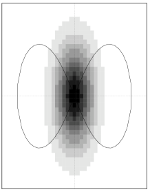
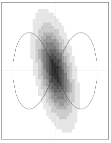
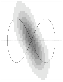
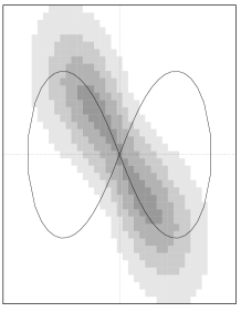
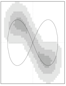
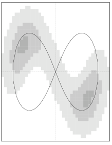
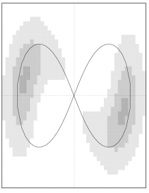
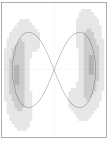
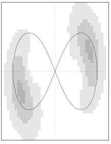
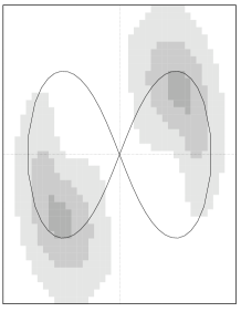
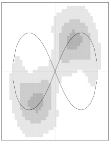
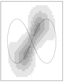
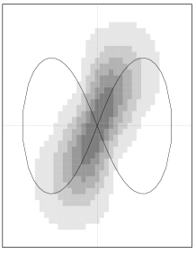
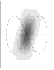
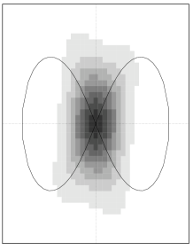
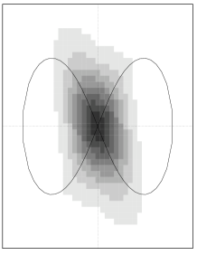
FIG. 6.: Evolution of a quantum state prepared at $t=0$ as Gaussian wave packet on the hyperbolic fixed point of the mixed quantum-classical dynamics ($p=2$, $r=0.1$, $\delta t=0.1$). The state is represented by the corresponding Husimi distribution after projection on the excitonic state $z=0$, $\phi=0$. The value of the Husimi distribution is encoded by the color using a linear scale with white corresponding to zero and black to one. The solid line is the isoenergy line of the lower adiabatic potential at the energy of the wave packet ($E=-0.5$), i. e. the separatrix associated with the hyperbolic fixed point in the adiabatic approximation.

FIG. 7.: Form of a Gaussian wave packet initially located at the hyperbolic fixed point for $p=2$ and $r=0.01$ at large time. Husimi distribution of the wave function projected on the excitonic state $z=0$, $\phi=0$ (left) and $z=1$ (right) in a surface plot.

  

FIG. 8.: Poincaré section $P=0$, $dP/dt>0$ for the symmetric dimer with $r=0.1$ and $p=2$ at $E=+0.5$. The circles mark the initial states, for which the time evolution will be displayed in the following figures. A regular island embedded into the chaotic sea has been enlarged in the lower part of the figure.

FIG. 9.: Time evolution of the initially factorized coherent state corresponding to A in fig. 8 ($\phi(t=0)=\pi$, $z(0)=-0.5$, $Q(0)=-1.2$, $E=0.55$). In the upper parts the quantum expectation values of $Q$ and $\sigma_{z}$ (full lines) are compared to the corresponding quantities of the mixed quantum-classical description (dashed lines). In the lower part the quantum Bloch radius $R(t)$ (53) is displayed using a larger time scale.

FIG. 10.: Time evolution of the initially factorized coherent state corresponding to B in fig. 8 ($\varphi(\tau=0)=0$, $z(0)=0$, $Q(0)=-14.1$, $E=0.55$). See fig. 9 for details.

FIG. 11.: Time evolution of the initially factorized coherent state corresponding to C in fig. 8 ($\varphi(\tau=0)=0$, $z(0)=0.9$, $Q(0)=-24.0$, $E=0.55$). See fig. 9 for details.

REFERENCES

- [1] Heller, E. J. In Giannoni, M. J., Voros, A. and Zinn-Justin, J., editors, ”Chaos and Quantum Physics”, Les Houches Summer School Sessions LII, North-Holland, Amsterdam, 1991.
- [2] Bohigas, O., Tomsovic, S., Ullmo, D.: Phys. Reports 223, 43 (1993).
- [3] Reinhardt, W. P.: Prog. Theor. Phys. Suppl. 116, 179 (1994).
- [4] Born, M., Huang, K.: ”Dynamical Theory of Crystal Lattices”, Oxford, Clarendon Press, 1954. Appendix VIII.
- [5] Bulgac, A., Kusnezov, D.: Chaos, Solitons & Fractals 5, 1051 (1995).
- [6] Blümel, R., Esser, B.: Phys. Rev. Lett. 72, 3658 (1994). Z. Phys. B 98, 119 (1995).
- [7] Sonnek, M., Eiermann, H., Wagner, M.: Phys. Rev. B 51, 905 (1995).
- [8] Graham, R., Höhnerbach, M.: Z. Phys. B 57, 233 (1984).
- [9] Kus, M.: Phys. Rev. Lett. 54, 1343 (1985).
- [10] Müller, L., Stolze, J., Leschke, H., Nagel , P.: Phys. Rev. A 44, 1022 (1991).
- [11] Esser, B., Schanz, H.: Chaos, Solitons & Fractals 4, 2067 (1994). Z. Phys. B 96, 553 (1995).
- [12] Schanz, H., Esser, B.: Z. Phys. B (in press).
- [13] Berman, P. B., Bulgakov, E. N., Holm, D. D.: Phys. Rev. A 49, 4943 (1994).
- [14] Cibils, M., Cuche, Y., Müller, G.: Z. Phys. B 97, 565 (1995).
- [15] Takahashi, K.: Progr. Theor. Phys. Suppl. Nr.98, 109 (1989).