Coupled Map Modeling for Cloud Dynamics

Abstract

A coupled map model for cloud dynamics is proposed, which consists of the successive operations of the physical processes; buoyancy, diffusion, viscosity, adiabatic expansion, fall of a droplet by gravity, descent flow dragged by the falling droplet, and advection. Through extensive simulations, the phases corresponding to stratus, cumulus, stratocumulus and cumulonimbus are found, with the change of the ground temperature and the moisture of the air. They are characterized by order parameters such as the cluster number, perimeter-to-area ratio of a cloud, and Kolmogorov-Sinai entropy.

PACS# 47.52.+j, 92.40.Cy, 92.60.Jq

Cloud dynamics plays an important role in the climate system, weather forecast, geophysics and so on. However this elementary process in meteorology is very much complicated because it consists of different time and space scales and the phase transition from liquid to gas is coupled with the motion of atmosphere. Even if the flow of the atmosphere were known with accuracy using Navier-Stokes equation, we could not discuss the morphology of cloud. In order to investigate such a complex system, construction of a phenomenological model is essential. In this letter, we introduce a coupled map lattice model of cloud formation which reproduces the diversity of cloud patterns. Characterizations of four cloud phases are also given.

Coupled map lattices (CML) are useful to study the dynamics of spatially extended systems [1]. Recently, CML has successfully been applied to spinodal decomposition [2], Rayleigh-Bénard convection [3], the boiling transition [4], and so on[5].

Here we construct a CML model of cloud in a 2-dimensional space. CML modeling is based on the separation and successive operation of procedures, which are represented as maps acting on a field variable on a lattice [6]. Here, we choose a two dimensional square lattice $(x,y)$ with $y$ as a perpendicular direction, and assign the velocity field $\vec{v}^{t}(x,y)$, the mass of the vapor $w_{v}^{t}(x,y)$ and the liquid $w_{\ell}^{t}(x,y)$, and the internal energy $E^{t}(x,y)$ as field variables at time $t$. The dynamics of these field variables consists of Lagrangian and Eulerian parts. For the latter part, we adopt the following processes ; (1) heat diffusion (2) viscosity (3) buoyance force (4) the pressure term requiring $div\vec{v}$ to be 0, in an incompressible fluid . Here, we use the discrete version of $grad(div\vec{v})$ which refrains from the growth of $div\vec{v}$. Indeed, we have already constructed the CML representations of the above four procedures [3]that agree with experiments on the Rayleigh-Bénard convection, which is a cardinal role for cloud dynamics. (5) diffusion of vapor $w_{v}^{t}(x,y)$; (6) adiabatic expansion; assuming the adiabatic process and the equilibrium ideal gas with gravity field, we adopt such an approximation that the temperature of the parcel risen from the height $y$ to $y+\Delta y$ is decreased in proportion to the displacement $\Delta y$. Thus the temperature $E^{t}(x,y)$ is decreased in proportion to $v_{y}^{t}(x,y)$. (7) phase transition from vapor $w_{v}^{t}(x,y)$ to liquid $w_{\ell}^{t}(x,y)$ and vise versa accompanied by the latent heat. Here, we use the simplest type of the bulk water-continuity model in meteorology [8]. The dynamics is represented as a relaxation to an equilibrium point $w^{*}(x,y)$ which is a function of temperature $E^{t}(x,y)$. (8) the dragging force; assuming that the droplets are uniform in size and fall with the terminal velocity $V$ with neglect of the relaxation time to it, the dragging force is proportional to the product of the relative velocity $(v_{y}^{t}(x,y)-V)$ and the density of droplets $w_{\ell}^{t}(x,y)$ at a lattice site.

Combining these dynamics, the Eulerian part is written as the successive operations of the following mappings (hereafter we use the notation for discrete Laplacian operator: $\Delta A(x,y)=\frac{1}{4}\{A(x-1,y)+A(x+1,y)+A(x,y-1)+A(x,y+1)-4A(x,y)\}$ for any field variable $A(x,y)$): For convenience, we represent state variables after an operation of each procedure with the superscript $t+1/n$ where $n$ is the total number of procedures.

Buoyancy and dragging force

$$v_{y}^{t+1/3}(x,y)=v_{y}^{t}(x,y)+\frac{c}{2}\{E^{t}(x+1,y)+E^{t}(x-1,y)-2E^{t}(x,y)\}-\gamma w_{\ell}(x,y)(v_{y}(x,y)-V)$$

Viscosity and pressure effect

$$\vec{v}^{t+2/3}(x,y) = \vec{v}^{t+1/3}(x,y)+\nu\Delta\vec{v}^{t+1/3}(x,y)+\eta grad(div\vec{v}^{t+1/3}(x,y))$$

with $grad(div\vec{v})$ as its discrete representation on the lattice [3].

Thermal diffusion and adiabatic expansion

$$E^{t+1/3}(x,y)=E^{t}(x,y)+\lambda\Delta E^{t}(x,y)-\beta v_{y}^{t}(x,y)$$

Diffusion of vapor

$$w_{v}^{t+1/3}(x,y))=w_{v}^{t}(x,y)+\lambda\Delta w_{v}^{t}(x,y)$$

Phase Transition To get the procedure, we use the discretized version of the following linear equations for the relaxation to equilibrium point $w^{*}$:

$$\frac{dw_{v}(x,y)}{dt} = +\alpha(w_{v}(x,y)-w^{*})$$

$$\frac{dw_{\ell}(x,y)}{dt} = -\alpha(w_{v}(x,y)-w^{*})$$

$$\frac{dE(x,y)}{dt} = -Q(\frac{dw_{v}(x,y)}{dt}-\frac{dw_{\ell}(x,y)}{dt})$$

$$w^{*}=\left\{\begin{array}[]{ll}A\exp(q/(E+const.))&\mbox{ if $>W(x,y)$}\\ W(x,y)&\mbox{otherwise}\end{array}\right.$$

which form is chosen to be consistent with the Clausius-Clapeyron’s equation exp(-q/Temperature) [9], while $W(x,y)=w_{\ell}(x,y)+w_{v}(x,y)$ is the total mass of water.

The Lagrangian scheme expresses the advection of velocity, temperature, liquid and vapor. This process is expressed by the motion of a quasi-particle on each lattice site $(x,y)$ with velocity $\vec{v}(x,y)$. We adopt the method presented in [3], while for the liquid variable $w_{\ell}(x,y)$, we also include the fall of a droplet with a final speed $V$. Thus, the quasi-particle moves to $(x+v_{x}(x,y),y+v_{y}(x,y)-V)$ to allocate $w_{\ell}(x,y)$ at its neighbors. Through this Lagrangian procedure, the energy and momentum are conserved.

Summing up, our dynamics is given by successive applications of the following step;

$$\left\{\begin{array}[]{c}\vec{v}^{t}(x,y)\\ E^{t}(x,y)\\ w^{t}(x,y)\end{array}\right\}\stackrel{{\scriptstyle\rm{Buoyancy+Dragging}}}{{\longmapsto}}\left\{\begin{array}[]{c}\vec{v}^{t+1/3}(x,y)\\ E^{t}(x,y)\\ w^{t}(x,y)\end{array}\right\}\stackrel{{\scriptstyle\rm{Viscosity+Pressure}}}{{\longmapsto}}\left\{\begin{array}[]{c}\vec{v}^{t+2/3}(x,y)\\ E^{t}(x,y)\\ w^{t}(x,y)\end{array}\right\}\stackrel{{\scriptstyle\rm{Diffusion}}}{{\longmapsto}}$$

$$\left\{\begin{array}[]{c}\vec{v}^{t+2/3}(x,y)\\ E^{t+1/3}(x,y)\\ w^{t+1/3}(x,y)\end{array}\right\}\stackrel{{\scriptstyle\rm{PhaseTransition}}}{{\longmapsto}}\left\{\begin{array}[]{c}\vec{v}^{t+2/3}(x,y)\\ E^{t+2/3}(x,y)\\ w^{t+2/3}(x,y)\end{array}\right\}\stackrel{{\scriptstyle\rm{Advection+Gravity}}}{{\longmapsto}}\left\{\begin{array}[]{c}\vec{v}^{t+1}(x,y)\\ E^{t+1}(x,y)\\ w^{t+1}(x,y)\end{array}\right\}$$

For the boundary, we choose the following conditions; (1) Bottom plates: Assuming the correspondence between $E$ and the temperature, we choose $E(x,0)=E_{0}$. (2) Top plates: We choose the no-flux condition $E_{t}(x,N_{y})-E_{t}(x,N_{y}-1)=0$. For both the plates, we choose the no-slip condition for the velocity field, and adopt the reflection boundary for the Lagrangian procedure. The liquid and vapor are fixed at zero for both the plates. (3) Side walls at $x=0$ and $x=N_{x}$: We use periodic boundary conditions.

The basic parameters in our model are the temperature $E_{0}$ at the ground, the Prandtl number (ratio of viscosity to heat diffusion $\nu/\lambda$), adiabatic expansion rate $\beta$, the terminal velocity of liquid droplets $V$, the coefficient for the dragging force $\gamma$, the phase transition rate $\alpha$, the latent heat $Q$ and the aspect ratio ($N_{x}/N_{y}$). Hereafter we fix these parameters as $\lambda=0.2,\eta=\nu=0.2,\beta=0.2,V=0.2,\gamma=0.2,\alpha=0.2,Q=0.2$, and study the change of the morphology in cloud as the ground temperature $E_{0}$ and the total mass of water $W=\sum_{x,y}(w_{v}(x,y)+w_{\ell}(x,y))$ are varied (note that $W$ is conserved).

To see the spatiotemporal dynamics, the evolution of the mass of the liquid $w_{\ell}(x,y)$ is studied. In Fig. 1, four typical time evolutions of $w_{\ell}(x,y)$ are plotted. By changing $E_{0}$ and $W$, the following four types of cloud have been found; (a) “stratus”, (b) “cumulus”, (c) “ stratocumulus” and (d) “cumulonimbus”.

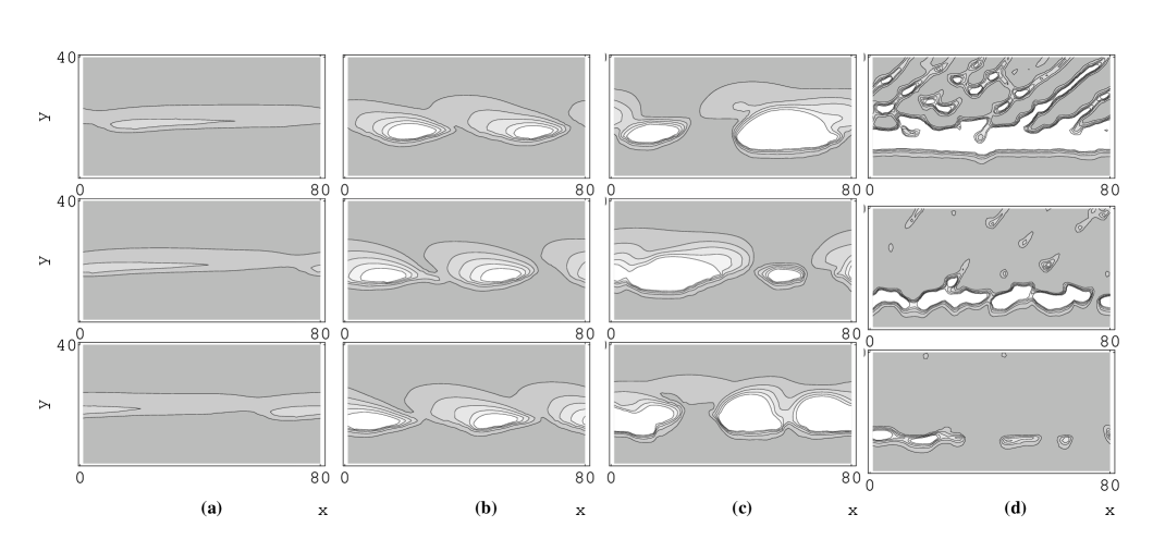
Figure 1:

Temporal evolution of cloud patterns. Snapshot of the mass of the liquid $w_{l}^{t}(x,y)$ is shown with the use of gray scale. The darker the pixel, the lower the liquid is. In other words, the white region corresponds to the high density of liquids, i.e., to a cloud region. Snapshot patterns are plotted from top to down per 200 steps after initial 5000 steps of transients, starting from a random initial condition. (a) Stratus ($E_{0}=3.0,W=0.006$), (b) Cumulus ($E_{0}=3.0,W=0.007$), (c) Cumulonimbus ($E_{0}=4.0,W=0.009$), (d) Stratocumulus($E_{0}=5.0,W=0.009$). The lattice size is $(N_{x},N_{y})=80\times 40$.

Stratus is a thin layered pattern of cloud, while cumulus is a thick lump of cloud. These two patterns are rather stable, while the other two patterns are dynamically unstable. At stratocumulus, a thin layered cloud pattern is torn into pieces and small fragments of clouds are scattered. These scattered clouds vanish while a new layered cloud is formed again later. The formation and annihilation of clouds are periodically repeated. Cumulonimbus is a thicker cloud in height than cumulus. Besides the size change, the cloud pattern is unstable. The clouds split and coalesce repeatedly. The classification into four types is based on the comparison between our spatiotemporal pattern and the definition by meteorology [8], while the phase diagram is given in Fig. 2, which is obtained from the pattern and quantifiers to be discussed. Summarizing the diagram, a cumulus or cumulonimbus is observed under the condition of rich moist air while a stratus appears in small $W$ and under low temperature.

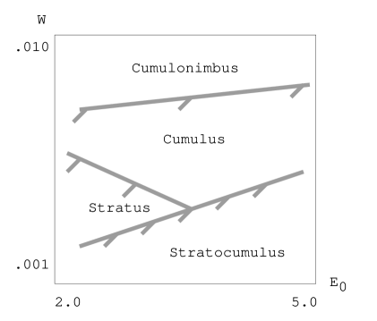
Figure 2:

Phase diagram for the morphology of cloud. The term stratus, cumulus, cumulonimbus and stratocumulus correspond to the pattern (a),(b),(c) and (d) in Fig. 1, respectively.

To classify these patterns quantitatively, we have measured several order parameters. First, we define a cloud cluster as connected lattice sites in which $w_{\ell}(x,y)$ is larger than a given threshold $w_{c}$. $C(t)$ is defined as the number of clusters disconnected with each other. Then, the “cloudiness” is measured by the total number of cloud sites, that is, $S(t)=\sum_{x=1}^{N_{x}}\sum_{y=1}^{N_{y}}\Theta(w_{\ell}(x,y)-w_{c})$, where $\Theta(x)$ is Heavisede function. The (temporal) average of the cluster number is large at the onset of cloud formation (i.e., small $E_{0}$ and $W$), and at the stratocumulus. The quantity $\langle S\rangle/\langle C\rangle$ measures the average size of each cloud cluster. It is larger at cumulus and is largest at cumulonimbus (Fig. 3-(a)).

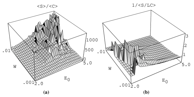
Figure 3:

(a) The average size of a cloud cluster $\langle S\rangle/\langle C\rangle$ and (b) the stratus order parameter (SOP), plotted with the change of $W$ and $E_{0}$. The average is taken over 20000 time steps after discarding 10000 steps of transients, starting from a random initial condition.

To characterize the difference between stratus and cumulus, the morphology of clouds should be taken into account. Roughly speaking, the stratus is a one-dimensional like pattern while the cumulus is a two-dimensional one. To see the morphological difference, we have measured the total perimeter of cloud $L(t)=\sum_{x=1,y=1}^{N_{x},N_{y}}\sum_{\delta x=\pm 1,\delta y=\pm 1}\Theta(w_{\ell}(x,y)-w_{c})\Theta(w_{c}-w_{\ell}(x+\delta x,y+\delta y))$. “Stratus order parameter” (SOP) is introduced as $\langle 1/(S(t)/(L(t)C(t)))\rangle_{t}$, the inverse of the ratio of area to perimeter per cluster. If it is large the pattern is close to a one-dimensional object. Change of SOP with $E_{0}$ and $W$ is plotted in Fig. 3(b). As is expected by the definition of SOP and the thin nature of stratus cloud, it has a larger value at the stratus phase and takes a lower value at the cumulus.

Of course, dynamical quantifiers are important to characterize the cloud patterns. For example, the fluctuations of the cluster size, SOP, and $S/C$ are larger at the cumulonimbus and stratocumulus phases. To see the dynamics closely, we have also measured the time series of the spatial sum of the mass of the liquid $\overline{L(t)}=\sum_{x,y}w_{\ell}^{t}(x,y)$, which corresponds to the cloudiness of the total space. The evolution of $\overline{L(t)}$ is almost stationary at stratus and cumulus, with only tiny fluctuations. The change is periodic at stratocumulus and chaotic at cumulus. It should be noted that the low-dimensional collective dynamics of the total liquid emerges even if the spatiotemporal dynamics is high-dimensional chaos.

To characterize chaotic dynamics, Kolmogorov-Sinai(KS) entropy is estimated by the sum of positive Lyapunov exponents, as is plotted in Fig. 4(b). It has a larger value at stratocumulus and cumulonimbus, which implies that the cloud dynamics there is chaotic both spatially and temporally. It is also positive at a lower temperature that corresponds to the onset of cloud formation, where the dynamics is unstable.

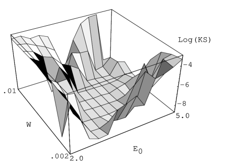
Figure 4:

KS entropy calculated by the sum of positive Lyapunov exponents is plotted versus $W$ and $E_{0}$. The first 20 Lyapunov exponents are computed by averaging over 20000 time steps after discarding initial 5000 steps.

In summary, we have proposed a CML model for pattern formation of cloud by introducing a simple phase transition dynamics from liquid to vapor, so called the bulk water-continuity model [8]. Our model reproduces the diversity of cloud patterns: stratus, stratocumulus, cumulus and cumulonimbus. This agreement implies that the qualitative feature of cloud dynamics is independent of microscopic details such as detailed droplet formation dynamics.

In order to globally understand the phenomenology, the present computationally efficient model is powerful, which makes us possible to characterize the cloud phases. We believe that the observed phase diagram for the morphology of the cloud is valid for the cloud in nature. It is also interesting to propose that similar phase changes may be seen generally in convective dynamics including phase transitions, since detailed processes specific only to clouds are abstracted in our model. Extensions of the present model to a three-dimensional case and inclusions of centrifugal and Coriolis forces are rather straightforward. By these extensions, study of the global atmosphere dynamics of a planet will be possible.

This work is partially supported by Grant-in-Aids for Scientific Research from the Ministry of Education, Science, and Culture of Japan, and by a cooperative research program at Institute for Statistical Mathematics.

References

- [1] K.Kaneko. Prog. Theor. Phys., 72:480, 1984.
- [2] Y.Oono S.Puri. Phys.Rev.Lett., 58:836, 1987.
- [3] T.Yanagita K.Kaneko. Physica D, 82:288, 1995.
- [4] T.Yanagita. Phys.Lett.A, 165:405, 1992.
- [5] Chaos Focus Issue on Coupled Map Lattice. CHAOS, 2, 1992.
- [6] K.Kaneko. in Formation, Dynamics and Statistics of Patterns I. World Scientific, 1990.
- [7] L.D.Landau E.M.Lifshitz. Fluid Mechanics, chapter 5. Pergamon, 1959.
- [8] R.A.Houze. Cloud Dynamics, volume 53 of Internatinal geophysics series. Academic Press, 1993.
- [9] L.D.Landau E.M.Lifshitz. Statistical Mechanics, chapter 8. Pergamon, 1958