Classical Kolmogorov scaling is inconsistent with local coupling

Abstract

We consider cascade models of turbulence which are obtained by restricting the Navier-Stokes equation to local interactions. By combining the results of the method of extended self-similarity and a novel subgrid model, we investigate the inertial range fluctuations of the cascade. Significant corrections to the classical scaling exponents are found. The dynamics of our local Navier-Stokes models is described accurately by a simple set of Langevin equations proposed earlier as a model of turbulence [Phys. Rev. E 50, 285 (1994)]. This allows for a prediction of the intermittency exponents without adjustable parameters. Excellent agreement with numerical simulations is found.

I Introduction

Much of our intuitive understanding of turbulence is based on the concept of interactions which are local in k-space. Physically, it is based on the notion that most of the distortion of a turbulence element or eddy can only come from eddies of comparable size. Turbulent features which are much larger only uniformly translate smaller eddies, which does not contribute to the energy transfer. This immediately leads to the idea of a chain of turbulence elements, through which energy is transported to the energy dissipating scales. Accepting such a cascade structure of the turbulent velocity field, it is natural to assume that the statistical average of velocity differences ${\bf\delta v(r)=v(x+r)-v(x)}$ over a distance $|{\bf r}|$ follows scaling laws

$$\left<|{\bf v(x+r)-v(x)}|^{p}\right>\sim r^{\zeta_{p}}$$ (1)

in the limit of high Reynolds numbers. By taking velocity differences over a distance $r$, one probes objects of corresponding size.

In addition to this assumption of self-similarity, Kolmogorov [1] also made the seemingly intuitive assumption that the local statistics of the velocity field should be independent of large-scale flow features, from which it is widely separated in scale. Because the turbulent state is maintained by a mean energy flux $\epsilon$, the only local scales available are the length $r$ and $\epsilon$ itself, which leads to the estimate $\delta v\sim(\epsilon r)^{1/3}$ or

$$\zeta^{(class)}_{p}=p/3\quad.$$ (2)

At the same time, one obtains an estimate for the Kolmogorov length

$$\eta=(\nu^{3}/\epsilon)^{1/4}$$ (3)

where viscosity is important. However, it was only appreciated later [2] that in turbulence long-range correlations always exist in spite of local coupling. Namely, large-scale fluctuations of the velocity field will result in a fluctuating energy transfer, which drives smaller scales. As a result, the statistics of the small-scale velocity fluctuations will be influenced by the energy transfer and fluctuations on widely separated scales are correlated, violating the fundamental assumption implicit in (2) and (3).

Indeed, Kolmogorov [3] and Obukhov [4] later proposed the existence of corrections to the scaling exponents (2),

$$\zeta_{p}=p/3+\delta\zeta_{p}\;,\delta\zeta_{p}\neq 0$$ (4)

which were subsequently confirmed experimentally [5, 6, 7, 8]. On one hand, careful laboratory experiments have been performed at ever higher Reynolds numbers [5, 9]. On the other hand, a new method of data analysis [6, 7] has been successful in eliminating part of the effects of viscosity. In particular, for the highest moments up to $p=18$ significant corrections to classical scaling were found, a currently accepted value for the so-called intermittency parameter $\mu$ being [5]

$$\mu=-\delta\zeta_{6}=0.2\quad,$$ (5)

which is a 10 % correction. The existence of corrections like (5) implies that on small scales large fluctuations are much more likely to occur than predicted by classical theory.

This “intermittent” behavior is thus most noticeable in derivatives of the velocity field such as the local rate of energy dissipation

$\displaystyle\epsilon({\bf x},t)=-\frac{\nu}{2}\left(\partial u_{i}/\partial x_{k}+\partial u_{k}/\partial x_{i}\right)^{2}\quad.$

Much of the research in turbulence has been devoted to the study of the spatial structure of $\epsilon({\bf x},t)$ [3, 10], but which will not be considered here. The statistical average of this quantity is what we simply called $\epsilon$ before. Owing to energy conservation, it must be equal to the mean energy transfer.

The local coupling structure of turbulence has inspired the study of so-called shell models, where each octave in wavenumber is represented by a constant number of modes, which are only locally coupled. This allows to focus on the implications of local coupling for intermittent fluctuations, disregarding effects of convection and mixing. The mode representation of a single shell serves as a simple model for the “coherent structures” a turbulent velocity field is composed of, and which to date have only been poorly characterized, both experimentally and theoretically.

We caution that this leaves out two important aspects of turbulence, both of which have recently been proposed to lie at the heart of intermittent behavior. First, we have assumed that coherent structure are simple in the sense that they only possess a single scale. But experimental [11], numerical [12], and theoretical [13] evidence points to the importance of long and skinny threads of vorticity. Although their real significance to turbulence is not without dispute [14], they have led to quantitative predictions of intermittency exponents [15], in excellent agreement with experiment. Second, nonlocal interactions are disregarded in shell models. On the other hand it has recently been proposed [16] in the framework of perturbation theory that non-local interactions can in fact be re-summed to yield correction exponents.

Given the complexity of the turbulence problem, this makes it all the more interesting to carefully assess the possibilities for intermittent fluctuations in the case where both effects are eliminated. Thus the aim of this paper is to combine previous numerical [17, 18] and analytical [19, 20] efforts to gain insight into intermittent fluctuations in models with local coupling alone. We focus on a particular class of shell models, introduced in [17], which establishes a direct connection with the Navier-Stokes equation. To this end the Navier-Stokes equation is projected on a self-similar selection of Fourier modes, which enforce local coupling. We will adopt the name REduced Wave vector set Approximation (REWA) here [18].

In the present paper, most of our effort is devoted to separating inertial range fluctuations from other effects relating to the fact that scale invariance is broken either by an external length scale $L$ or by the Kolmogorov length $\eta$. To this end we simulate extremely long cascades, covering up to 5 decades in scale. To eliminate viscous effects as much as possible, we use the method of extended self-similarity (ESS) [6, 7]. In addition, to make sure our results are independent of the method of data analysis, we develop a new subgrid model using fluctuating eddy viscosities [21]. The results are in excellent agreement with those found from ESS. Finally, and perhaps most importantly, we use an analytical calculation [20] to predict the correction exponent without adjustable parameters. Again, we find the same values within error bars. We show that the stochastic model introduced in [19] gives an excellent description of a REWA cascade, both in an equilibrium and non-equilibrium state. We compare the equilibrium properties to adjust a single free parameter in the stochastic model.

Thus we reach two objectives: First, we gain analytical insight into the origin of intermittent fluctuations in a local cascade. Second, we demonstrate for a simple example how equilibrium information about the interactions of Fourier modes can be used to compute intermittency exponents.

Unlike shell models with only one complex mode per shell [23, 24, 25] exponent corrections $\delta\zeta_{p}$ for REWA cascades are quite small [17, 18]. Careful studies of inertial range fluctuations have found them to be significant [18], but their numerical value is only about 1/10 of the numbers found experimentally [5]. This has lead to the idea that perhaps the experimentally observed exponent corrections are not genuine inertial range properties, but result from extrapolations of (1) into regimes where stirring or viscous effects are important [17, 18, 26].

We will not follow up on this idea here. However, we note that the REWA cascade misses an essential feature of three-dimensional turbulence and thus can hardly be expected to yield quantitative predictions. Namely, in real turbulence, the number of modes within a shell proliferates like $r^{-2}$ as one goes to smaller scales, while in cascade models this number is constant. This can be remedied by allowing a particular shell to branch out into eight sub-shells, which represent eddies of half the original size. It has been argued [27, 19] that the competition between eddies of the same size is responsible for the much larger growth of fluctuations observed in three-dimensional turbulence. The difficulty with this approach is that one also has to take convection of spatially localized structures into account. Also, it is not obvious how to disentangle interactions which are local in $k$-space from those local in real space, as to systematically reduce the coupling of the Navier-Stokes equation to a tree of turbulence elements. Recently developed wavelet methods are a promising step [28], but they have so far been used only for data analysis [29].

The paper is organized as follows: In the next section we introduce both the mode-reduced approximations of the Navier-Stokes equation and the corresponding Langevin models. The inertial range properties of the latter have only one adjustable parameter, as explained in the third section. This parameter is determined for a given selection of Fourier modes by considering the equilibrium fluctuations of both models. We are thus able to predict intermittency exponents of the turbulent state without adjustable parameters. The result is compared with numerical simulations of the REWA cascades in the fourth section. Exponents are determined by carefully examining various sources of error, and are in excellent agreement with the theoretical prediction. In the fifth section, we investigate temporal correlations in REWA models to inquire further in the origin of intermittency in models with local coupling. This also sheds light on the reasons for the success of the simple Langevin model used by us.

II Two cascade models

A Reduced wave vector set approximation

The REWA model [17, 18] is based on the full Fourier–transformed Navier–Stokes equation within a volume of periodicity $(2\pi L)^{3}$. In order to restrict the excited Fourier–modes of the turbulent velocity field to a numerically tractable number, the Navier–Stokes equation is projected onto a self–similar set of wave vectors ${\cal K}=\bigcup_{\ell}{\cal K}_{\ell}$. Each of the wave vector shells ${\cal K}_{\ell}$ represents an octave of wave numbers. The shell ${\cal K}_{0}$ describes the turbulent motion of the large eddies which are of the order of the outer length scale $L$. This shell is defined by $N$ wave vectors ${\bf k}^{(0)}_{i}$: ${\cal K}_{0}=\{{\bf k}^{(0)}_{i}:i=1,\dots,N\}$. Starting with the generating shell ${\cal K}_{0}$, the other shells ${\cal K}_{\ell}$ are found by a successive rescaling of ${\cal K}_{0}$ with a scaling factor 2: ${\cal K}_{\ell}=2^{\ell}{\cal K}_{0}$. Thus each ${\cal K}_{\ell}$ consists of the $N$ scaled wave vectors $2^{\ell}{\bf k}_{i}^{(0)},\ i=1,\dots,N$. The shell ${\cal K}_{\ell}$ represents eddies at length scales $r\sim 2^{-\ell}L$, i.e. to smaller and smaller eddies as the shell index $\ell$ increases. At scales $r\approx\eta$ the fluid motion is damped by viscosity $\nu$, thus preventing the generation of infinitely small scales. Hence we only need to simulate shells ${\cal K}_{\ell},\ell<\ell_{\nu}$, where $\ell_{\nu}\approx\log_{2}(L/\eta)$ is chosen such that the amplitudes in ${\cal K}_{\ell_{\nu}}$ are effectively zero. In this representation the Navier–Stokes equation for incompressible fluids reads for all ${\bf k}\in{\cal K}=\bigcup_{\ell=0}^{\ell_{\nu}}{\cal K}_{\ell}$:

$$\frac{\partial}{\partial t}u_{i}({\bf k},t) = -\imath M_{ijk}({\bf k})\sum_{{\bf p},{\bf q}\in{\cal K}\atop{\bf k}={\bf p}+{\bf q}}u_{j}({\bf p},t)u_{k}({\bf q},t)-\nu k^{2}u_{i}({\bf k},t)+f_{i}({\bf k},t)$$ (7)

$${\bf k}\cdot{\bf u}({\bf k},t) = 0\quad.$$ (8)

The coupling tensor $M_{ijk}({\bf k})=\left[k_{j}P_{ik}({\bf k})+k_{k}P_{ij}({\bf k})\right]/2$ with the projector $P_{ik}({\bf k})=\delta_{ik}-k_{i}k_{k}/k^{2}$ is symmetric in $j,k$ and $M_{ijk}({\bf k})=-M_{ijk}(-{\bf k})$. The inertial part of equation (7) consists of all triadic interactions between modes with ${\bf k}={\bf p}+{\bf q}$. They are the same as in the full Navier-Stokes equation for this triad. The velocity field is driven by an external force ${\bf f}({\bf k},t)$ which simulates the energy input through a large-scale instability.

Within this approximation scheme the energy of a shell is

$$E_{\ell}(t)=\frac{1}{2}\sum_{{\bf k}\in{\cal K}_{\ell}}|{\bf u}({\bf k},t)|^{2}\quad,$$ (9)

and in the absence of any viscous or external driving the total energy of the flow field $E_{tot}(t)=\sum_{\ell=0}^{\ell_{\nu}}E_{\ell}(t)$ is conserved. The choice of generating wave vectors ${\bf k}^{(0)}_{i}$ determines the possible triad interactions. This choice must at least guarantee energy transfer between shells and some mixing within a shell. In [17, 18] different choices for wavenumber sets ${\cal K}_{0}$ are investigated. The larger the number $N$ of wave numbers, the more effective the energy transfer. Usually one selects directions in ${\bf k}$-space to be distributed evenly over a sphere. However, there are different possibilities which change the relative importance of intra-shell versus inter-shell couplings. In this paper, we are going to investigate two different wave vector sets, with $N=26$ and $N=74$, which we call the small and the large wave vector set, respectively. In Fig. 1 a two-dimensional projection of both sets is plotted. The large wave vector set also contains some next-to-nearest neighbor interactions between shells, which we put to zero here, since they contribute little to the energy transfer. The small set allows 120 different interacting triads, the large set 501 triads, 333 of which are between shells.

=0.4

FIG. 1.: A two-dimensional projection of the $k$-vectors in shell ${\cal K}_{0}$ for both the REWA models considered here. The small set ($\times$) contains all vectors with -1, 0, and 1 as components. The large set ($\bigcirc$), in addition, contains combinations with $\pm 1/2$ and $\pm 2$.

Since in the models we consider energy transfer is purely local, the shell energies $E_{\ell}(t),\ \ell=0,\dots,\ell_{\nu}$ only change in response to energy influx $T_{\ell-1\rightarrow\ell}$ from above and energy outflux $T_{\ell\rightarrow\ell+1}$ to the lower shell. In addition, there is a rate of viscous dissipation $T_{\ell}^{(diss)}(t)$ which is concentrated on small scales, and a rate of energy input $T_{0}^{in}(t)$, which feeds the top level only, cf. Fig.2.

=0.2

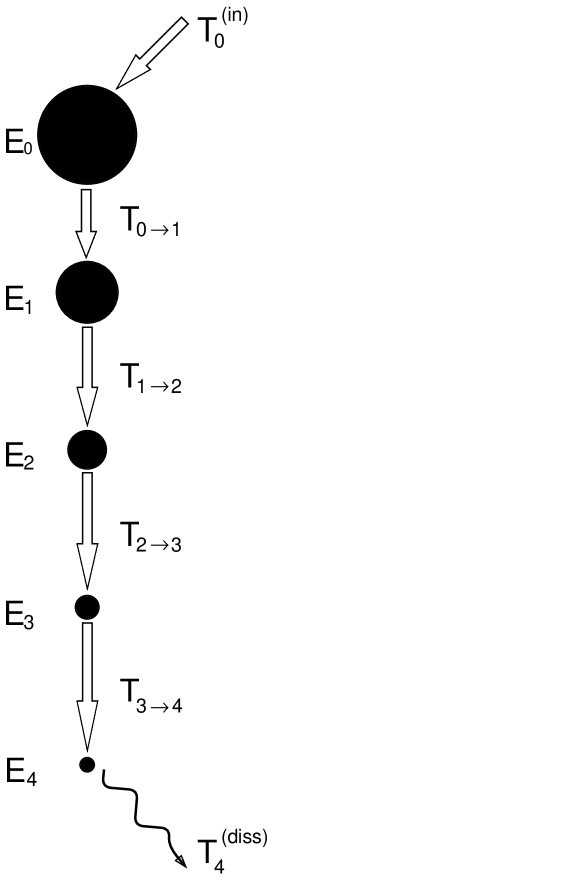
FIG. 2.: The structure of a local cascade. Eddies of size $r\sim 2^{-\ell}L$ are represented by their total energy $E_{\ell}$. Only modes of neighboring shells interact, leading to a local energy transfer $T_{\ell\rightarrow\ell+1}(t)$. The cascade is driven by injecting energy into the largest scale with rate $T_{0}^{(in)}(t)$. The turbulent motion is damped by viscous dissipation at a rate $T_{\ell}^{(diss)}(t)$.

From equation (7) we find an energy balance equation which governs the time evolution of the shell energies $E_{\ell}(t)$

$$\frac{d}{dt}E_{\ell}(t)=T_{\ell-1\rightarrow\ell}(t)-T_{\ell\rightarrow\ell+1}(t)+T_{\ell}^{(diss)}(t)+T_{0}^{(in)}(t)\delta_{\ell 0}\quad.$$ (10)

The different transfer terms are found to be

$$T_{\ell\rightarrow\ell+1}(t) = 2\imath\sum_{\triangle^{(\ell+1)}_{(\ell)}}M_{ijk}({\bf k})u_{i}^{*}({\bf k},t)u_{j}({\bf p},t)u_{k}({\bf q},t)$$ (12)

$$T_{0}^{(in)}(t) = \sum_{{\bf k}\in{\cal K}_{0}}\mbox{\rm Re}\left({\bf u}^{*}({\bf k},t)\cdot{\bf f}({\bf k},t)\right)$$ (13)

$$T_{\ell}^{(diss)}(t) = -\nu\sum_{{\bf k}\in{\cal K}_{\ell}}k^{2}|{\bf u}({\bf k},t)|^{2}\quad.$$ (14)

In equation (12) $\sum_{\triangle^{(\ell+1)}_{(\ell)}}$ indicates the summation over all next–neighbor triads ${\bf k}={\bf p}+{\bf q}$ with ${\bf k}\in{\cal K}_{\ell},\ {\bf p}\in{\cal K}_{\ell+1}$ and ${\bf q}\in{\cal K}_{\ell}\bigcup{\cal K}_{\ell+1}$.

The driving force ${\bf f}({\bf k},t)$ is assumed to act only on the largest scales, and controls the rate of energy input $T_{0}^{(in)}(t)$. As in Reference [17] we choose ${\bf f}({\bf k},t)$ to ensure constant energy input $T^{(in)}_{0}=\epsilon$ :

$${\bf f}({\bf k},t) = \frac{\epsilon{\bf u}({\bf k},t)}{2N|{\bf u}({\bf k},t)|^{2}}\enspace\mbox{for all }{\bf k}\in{\cal K}_{0}$$ (16)

$${\bf f}({\bf k},t) = 0\enspace\mbox{for all }{\bf k}\not\in{\cal K}_{0}\quad.$$ (17)

This leads to a stationary cascade whose statistical properties are governed by the complicated chaotic dynamics of the nonlinear mode interactions. Owing to energy conservation, viscous dissipation equals the energy input on average. The Reynolds number is given by

$$Re=\frac{LU}{\nu}=\frac{\epsilon L^{2}}{\left<E_{0}\right>\nu}\quad,$$ (18)

since $T=\left<E_{0}\right>/\epsilon$ sets a typical turnover time scale of the energy on the highest level. We believe $T$ to be of particular relevance, since the large-scale fluctuations of the energy will turn out to be responsible for the intermittent behavior we are interested in. In [18], for example, time is measured in units of $L^{2/3}\epsilon^{-1/3}$, which typically comes out to be 1/10th of the turnover time of the energy $T$. As we are going to see below, this is rather a measure of the turnover times of the individual Fourier modes. Figure 3 shows the scaling of the mean energy in a log-log plot at a Reynolds number of $4.2\cdot 10^{5}$. The inertial range extends over three decades, where a power law very close to the prediction of classical scaling is seen. Below the 10th level the energies drop sharply due to viscous dissipation. In Section III we are going to turn our attention to the small corrections to 2/3-scaling, hardly visible in Fig. 3. Still, there are considerable fluctuations in this model, as evidenced by the plot of the energy transfer in Fig. 4. Typical excursions from the average, which is normalized to one, are quite large. Ultimately, these fluctuations are responsible for the intermittency corrections we are going to observe.

=0.4

FIG. 3.: Log–log–plot of the structure function $\tilde{D}_{\ell}^{(2)}=\left<E_{\ell}\right>$ versus level number for the small cascade. At large scales, where the influence of dissipation is negligible, classical scaling is observed. At small scales the turbulent motion is damped by viscosity. The Reynolds number is $Re=4.2\cdot 10^{5}$.

=0.4

FIG. 4.: Time evolution of the energy transfer $T_{0\rightarrow 1}(t)$ from shell ${\cal K}_{0}$ to shell ${\cal K}_{1}$. Typical excursions are large compared with the mean value $\left<T_{0\rightarrow 1}\right>=\epsilon$. The time is given in units of $T=\left<E_{0}\right>/\epsilon$, where $\left<E_{0}\right>$ is the mean energy of the top level.

Thus within the REWA–cascade we are able to numerically analyze the influence of fluctuations on the stationary statistical properties of a cascade with local energy transfer on the basis of the Navier–Stokes equation. In Fig. 5 we plot the time evolution of the energy on the second level of the cascade. One observes

=0.4

FIG. 5.: Energy of a shell ($\ell=2$) as a function of time. The rapid fluctuations come from the motion of individual Fourier modes. A much longer time scale is revealed by performing a floating average over one turnover time of the second level (bold line). The time is given in units of $T=\left<E_{0}\right>/\epsilon$.

short-scale fluctuations, which result from the motion of individual Fourier modes within one cascade level. However, performing a floating average reveals a second time scale, which is of the same order as the turnover time of the top level. As we are going to see in Section IV, this disparity of time scales is even more pronounced on lower levels. The physics idea is the same as in the microscopic foundation of hydrodynamics, where conserved quantities are assumed to move on much slower time scales than individual particles. This motivates us to consider the energy as the only dynamical variable of each shell, and to represent the rapid fluctuations of Fig. 5 by a white-noise Langevin force. In this approximation we still hope to capture the rare, large-scale events characteristic of intermittent fluctuations, since the conserved quantity is the “slow” variable of the system. Similar ideas have also been advanced for the conservative dynamics of a non-equilibrium statistical mechanical system [30].

B The Langevin–cascade

In this model we take a phenomenological view of the process of energy transfer. The chaotic dynamics of the REWA cascade is modeled by a stochastic equation. We make sure to include the main physical features of energy conservation and local coupling. In particular, the dynamics is simple enough to allow for analytical insight into the effects of fluctuating energy transfer [20].

As in the preceding REWA–cascade, the turbulent flow field is described by a sequence of eddies decaying successively (Figure 2). The eddies at length scales $r\sim 2^{-\ell}L$ are represented by their energy $E_{\ell}(t)$. As before we restrict ourselves to local energy transfer, and thus the time evolution of the shell energies $E_{\ell}(t)$ is governed by equation (10). The crucial step is of course to choose an appropriate energy transfer $T_{\ell\rightarrow\ell+1}(t)$. For simplicity, we restrict ourselves to a Langevin process with a white noise force. Thus the local transfer $T_{\ell\rightarrow\ell+1}(t)$ is split into a deterministic and a stochastic part $T_{\ell\rightarrow\ell+1}(t)=T_{\ell\rightarrow\ell+1}^{(det)}(t)+T_{\ell\rightarrow\ell+1}^{(stoch)}(t)$ where both parts should depend only on the local length scale $2^{-\ell}L$ and the neighboring energies $E_{\ell}$ and $E_{\ell+1}$. The most general form dimensionally consistent with this has been given in [20]. For simplicity, here we restrict ourselves to the specific form

$$T_{\ell\rightarrow\ell+1}^{(det)}(t) = D\frac{2^{\ell}}{L}\left(E_{\ell}^{3/2}(t)-E_{\ell+1}^{3/2}(t)\right)$$ (20)

$$T_{\ell\rightarrow\ell+1}^{(stoch)}(t) = R\left(\frac{2^{(\ell+1)}}{L}\right)^{1/2}E_{\ell}^{5/8}(t)E_{\ell+1}(t)^{5/8}\xi_{\ell+1}(t)$$ (21)

$$T_{\ell}^{(in)}(t) = \epsilon\delta_{\ell 0}$$ (22)

$$T^{(diss}_{\ell}(t) = -\nu(2^{-\ell}L)^{-2}E_{\ell}\quad.$$ (23)

The white noise is represented by $\xi_{\ell}$, i.e. $\left<\xi_{\ell}(t)\right>=0$ and $\left<\xi_{\ell}(t)\xi_{\ell^{\prime}}(t^{\prime})\right>=2\delta_{\ell\ell^{\prime}}\delta(t-t^{\prime})$. We use Ito’s [31] definition in equation (21). To understand the dimensions appearing in (II B), note that $u_{\ell}\sim E_{\ell}^{1/2}$ is a local velocity scale and $k\sim 2^{\ell}/L$ is a wavenumber. Thus (20) dimensionally represents the energy transfer (12). In (21) the powers are different, since $\xi$ carries an additional dimension of $1/\mbox{time}^{1/2}$. It follows from (20) that the sign of the deterministic energy transfer depends on which of the neighboring energies $E_{\ell}$ or $E_{\ell+1}$ are greater. If for example $E_{\ell}$ is larger, $T^{(det)}_{\ell\rightarrow\ell+1}(t)$ is positive, depleting $E_{\ell}$ in favor of $E_{\ell+1}$. Hence the deterministic part tends to equilibrate the energy among the shells. The stochastic part, on the other hand, is symmetric with respect to the two levels $\ell$ and $\ell+1$. This reflects our expectation that in equilibrium it is equally probable for energy to be scattered up or down the cascade.

The combined effect of (20) and (21) is that without driving, energies fluctuate around a common mean value. This equipartition of energy in equilibrium is precisely what has been predicted on the basis of the Navier-Stokes equation [32, 33]. The only free parameters appearing in the transfer are thus the amplitudes $D$ and $R$. If $R$ is put to zero, the motion is purely deterministic, and one obtains the simple solution

$$E_{\ell}^{(0)}=C2^{-(2/3)\ell}\ \mbox{with}\ C=\left(\frac{2\epsilon L}{D}\right)^{2/3}\quad.$$ (24)

This corresponds to a classical Kolmogorov solution with no fluctuations in the transfer. The amplitude $D$ of the deterministic part is a measure of the effectiveness of energy transfer. On the other hand $R$ measures the size of fluctuations. In [20] it is shown that a finite $R$ necessarily leads to intermittency corrections in the exponents. In the next section we are going to determine the model parameters for the two REWA cascades we are considering.

III Determination of model parameters

The aim of this section is to explain the significance of the parameters appearing in the Langevin model. We show that only the combination $R/D^{1/2}$ determines the nonequilibrium fluctuations in the inertial range. But it is the same combination which also sets the width of the equilibrium distribution of energies, if the chain of shells is not driven. Thus we are able to fix all the parameters necessary to describe the nonequilibrium state solely by measuring equilibrium properties.

The physical parameters of the turbulent cascade are the length scale $L$ of the highest level, the rate of energy input $\epsilon$, and the viscosity $\nu$. The properties of the energy transfer are determined by the dimensionless strength of the deterministic part $D$ and of the stochastic part $R$. In the previous section we have seen that $E^{(0)}_{0}=(2\epsilon L/D)^{2/3}$ sets an energy scale for the highest level, and thus $T=E^{(0)}_{0}/\epsilon$ is a time scale. Both scales can be used to non-dimensionalize (II B), giving

$$\hat{T}_{\ell\rightarrow\ell+1}^{(det)}(t) = 2^{\ell+1}\left(\hat{E}_{\ell}^{3/2}(t)-\hat{E}_{\ell+1}^{3/2}(t)\right)$$ (26)

$$\hat{T}_{\ell\rightarrow\ell+1}^{(stoch)}(t) = \frac{R}{D^{1/2}}2^{(\ell+2)/2}\hat{E}_{\ell}^{5/8}(t)\hat{E}_{\ell+1}(t)^{5/8}\hat{\xi}_{\ell+1}(t)$$ (27)

$$\hat{T}_{0}^{(in)}(t) = 1$$ (28)

$$\hat{T}_{\ell}^{(diss)}(t) = -2^{2\ell}(Re)^{-1}\hat{E}_{\ell}\quad.$$ (29)

Hence $R/D^{1/2}$ is the only parameter characterizing the inertial range dynamics, which can be understood as follows: At any level $\ell$, a time scale of deterministic transport is set by $\tau_{D}\sim E_{\ell}/\epsilon\sim E_{\ell}^{-1/2}r/D$, where $E_{\ell}$ is a typical energy scale and $r=2^{-\ell}L$. This deterministic transport competes with diffusion of energy introduced by the stochastic part of the energy transfer. Namely a time scale over which the energy $E_{\ell}$ can diffuse away is given by $\tau_{R}\sim(E_{\ell}/A)^{2}$, where $A=R\epsilon r^{-1/2}E_{\ell}^{3/4}$ is the amplitude of the noise term. Plugging in the expression from (21) one ends up with $\tau_{R}\sim rE_{\ell}^{-1/2}/R^{2}$, and hence

$\displaystyle\frac{\tau_{R}}{\tau_{D}}\sim\frac{D}{R^{2}}.$

In particular, the relative importance of deterministic transport and diffusion is independent of the level, and only depends on the combination of $D$ and $R$ given above.

We are now left to determine $R/D^{1/2}$ from an experiment which is independent of the nonequilibrium state. To that end we consider a long chain of shell elements, for which energy input as well as viscous dissipation has been turned off ($\epsilon=\nu=0$). As a result, the energy will perform fluctuations around some mean value $\left<E_{\ell}\right>$. Using a similar argument as above, the probability distribution $p(E_{\ell}/\left<E_{\ell}\right>)$ for the shell energies will only depend on $R/D^{1/2}$ for the Langevin model. Figure 6 shows the probability distribution for one level of a cascade with 7 shells. Except for some end effects at the lowest level, the distribution turns out to be level-independent. The large REWA cascade is compared

=0.4

FIG. 6.: Equilibrium distribution of the energy in the top level of the large REWA–cascade ($N=74$), consisting of 7 shells. By adjusting the only parameter $R/D^{1/2}$, the distribution of the Langevin cascade can be made to agree within statistical error. The results for $R/D^{1/2}$ for both wave vector sets are given in (6).

with a simulation of the Langevin cascade. Once $R/D^{1/2}$ is adjusted, there is an almost perfect match between the two models. This shows that the simple stochastic dynamics proposed here models the equilibrium distribution of the chaotic fluctuations of Fourier modes very well. Most importantly, we have determined the only adjustable parameter of the energy transfer of the Langevin cascade corresponding to the two model systems we are considering:

$$\frac{R}{D^{1/2}} =1.729\cdot 10^{-1} \mbox{ for the small cascade}\;(N=26),$$ (32)

$$\frac{R}{D^{1/2}} =9.968\cdot 10^{-2} \mbox{ for the large cascade}\;(N=74)\quad.$$ (33)

As seen from (6), the REWA cascade with a larger number of modes has smaller fluctuations. This is not surprising, since large excursions of the energy correspond to a coherent motion of the individual Fourier modes. The larger the number of modes, the harder this is to achieve, since the random motion of individual modes tends to destroy correlations.

In the next section, the fit (32),(33) will be used to compare nonequilibrium properties in the inertial range. All information about possible differences between the small and the large cascade has been condensed into a single number.

IV Intermittency Corrections

We now turn to the inertial range fluctuations of the two cascade models. To allow for a direct comparison, we focus on the scaling of the energies $E_{\ell}$ of one shell. The analogue of the moments of the velocity field usually considered in turbulence are the structure functions based on the energy

$$\tilde{D}^{(p)}_{\ell}=\left<E_{\ell}^{p/2}\right>\sim 2^{-\zeta_{p}\ell}\quad.$$ (34)

We concentrate on the small corrections $\delta\zeta_{p}$ to the scaling exponents as predicted on dimensional grounds. As seen in Fig. 3, these corrections are extremely small, so that no significant deviation from classical scaling is seen on the scale of the figure.

In order to know what to expect, we use the result of Ref. [20] where we have computed the scaling behavior of a general class of stochastic models in a perturbation expansion. To lowest order, the exponent corrections are given by the quadratic dependence

$$\delta\zeta_{p}=-\mu\frac{p}{18}(p-3)\quad.$$ (35)

Plugging the specific form of the energy transfer (26), (27) into the formulae given in [20], we find

$$\mu=0.42\left(\frac{R}{D^{1/2}}\right)^{2}\quad.$$ (36)

For the small cascade this leads to $\mu=0.013$, which is about 1/10 of the experimental value accepted for three-dimensional turbulence [5]. Therefore, it is more than ordinarily difficult to measure the scaling exponents with sufficient accuracy to obtain significant answers for the deviations from classical scaling. On the other hand, the number of modes in a REWA cascade being greatly reduced as compared with the full Navier-Stokes equation, we are able to simulate cascades with up to 17 levels, corresponding to 5 decades in scale.

To obtain reliable results within the accuracy needed, it is essential to disentangle statistical errors from systematic errors, introduced through finite-size effects or viscous damping. To that end we individually assign statistical errors to every average taken. Figure 7

=0.4

FIG. 7.: Convergence of the structure function $\tilde{D}_{\ell}^{(18)}=\left<E_{\ell}^{9}\right>$, on the 11th step of the small REWA cascade. We show the evolution of $\tilde{D}_{\ell}^{(18)}$ as function of the averaging time $T_{av}$ in comparison with the stationary values $\tilde{D}_{\ell}^{(18,stat)}$, which are calculated by integrating over all initial values in the data set. The error bars give the statistical error of the data as estimated by (37). The averaging time $T_{av}$ is given in units of $T=\left<E_{0}\right>/\epsilon$.

shows the convergence of the 9th moment of the energy on the 11th step of the small REWA cascade, which is the lowest level relevant to our fits. We plot the mean value, averaged over the time given. Evidently the fluctuations of this mean value get smaller as the averaging time $T_{av}$ is increased. To obtain a quantitative measure of the uncertainty of the $T$-average of some quantity $x$, we also consider the ensemble of averages obtained with different initial conditions. The result for the mean value and variance of this ensemble average is plotted as circles with error bars in Fig. 7, where $E_{\ell}^{9}$ takes the place of $x$. The variance is found equivalently as an integral over the temporal correlation function [34]:

$$\sigma_{x}^{2}(T_{av})=\frac{1}{T_{av}^{2}}\int^{T_{av}}_{0}\int^{T_{av}}_{0}\left[\left<x(\tau_{1})x(\tau_{2})\right>-\left<x\right>^{2}\right]d\tau_{1}d\tau_{2}\quad.$$ (37)

This variance $\sigma(T_{av})$ is seen to give a reasonable approximation to the fluctuations of the temporal average. The variance for the largest averaging time available has been taken as the statistical error of a measured temporal average.

Next we consider systematic errors in the computation of the scaling exponents. Deviations from power law scaling are expected to occur on both ends of the cascade and have been studied extensively [17, 35, 18]. First, fluctuations on the highest level are suppressed, since there is no coupling to a higher level, but deterministic energy input instead. Second, in the viscous subrange the energy is increasingly depleted by viscosity, leading to even more drastic effects on the spectra. Both effects are strongest for the highest moments, which are most sensitive to large fluctuations. The 18th order structure function for a typical run of the small cascade is plotted as diamonds in Fig. 8. The average on the highest level is considerably lower than expected from scaling, as fluctuations are suppressed.

=0.4

FIG. 8.: Scaling of the structure functions $\tilde{D}_{\ell}^{(p)}=\left<E_{\ell}^{p/2}\right>$ with $p=3$ ($\bigcirc$) and $p=18$ ($\Diamond$) versus level number (Standard) in comparison with extended self similarity (ESS) scaling of $\tilde{D}_{\ell}^{(18)}$ ($\Box$) versus $\tilde{D}_{\ell}^{(3)}/\tilde{D}_{0}^{(3)}$. The structure functions are normalized by their power law fits: $\tilde{D}_{\ell}^{(p,norm)}=\tilde{D}_{\ell}^{(p)}/(b^{(p)}2^{-\zeta_{p}\ell})$ in the standard plot and $\tilde{D}_{\ell}^{(p,norm)}=\tilde{D}_{\ell}^{(p)}/(A^{(p)}(\tilde{D}_{\ell}^{(3)}/\tilde{D}_{0}^{(3)})^{\zeta_{p}/\zeta_{3}})$ in the ESS plot. Refer to Table I for the values of the exponents. In the ESS plot the scaling range is more than doubled. The numerical calculation is performed for the small REWA cascade.

The cascade only gradually recovers from this suppression, which leads to a faster rise in the level of fluctuations and thus to a decrease in the local scaling exponent as reported in [18]. Note that we show a “scatter-plot” of the data around the power law $\tilde{D}^{(p)}_{\ell}\sim 2^{-\ell\zeta_{p}}$, which represents our best fit. Thus deviations from this power law are hugely exaggerated and would not be visible on a customary log-log-plot. The absolute variation of $\tilde{D}^{(18)}_{\ell}$ over the range of the plot is 21 orders of magnitude. Owing to the extreme sensitivity of our plot, viscous damping is visible below the fourth level, even for a cascade with 17 shells, as seen in Fig. 8. This restricts the inertial range to four levels. We employ two different strategies to improve on this situation: (i) We plot the higher order structure functions against the third order structure function, as suggested by the ESS method. (ii) We eliminate viscosity altogether by introducing a fluctuating eddy viscosity instead.

It is known [6, 7] that extended self-similarity leads to a very considerable improvement of the scaling of experimental data. Without any viscous corrections, the scaling behavior is unaffected, as seen in Fig. 8 in the fitting range marked “standard”. Below the forth level, however, the third order structure function suffers viscous damping quite similar to that affecting the other structure functions.

p	$\delta\zeta_{p}$ (ESS)				$\delta\zeta_{p}$ (EV)				$\delta\zeta_{p}$ (Theory)
2	$1.5$⋅	$10^{-3}$ ${}\pm{}$	$1.5$⋅	$10^{-3}$	$1.4$⋅	$10^{-3}$ ${}\pm{}$	$2$⋅	$10^{-4}$	$1.4$⋅	$10^{-3}$
6	$-1.3$⋅	$10^{-2}$ ${}\pm{}$	$5$⋅	$10^{-3}$	$-1.3$⋅	$10^{-2}$ ${}\pm{}$	$1$⋅	$10^{-3}$	$-1.3$⋅	$10^{-2}$
12	$-7.5$⋅	$10^{-2}$ ${}\pm{}$	$1$⋅	$10^{-2}$	$-7.4$⋅	$10^{-2}$ ${}\pm{}$	$2$⋅	$10^{-3}$	$-7.6$⋅	$10^{-2}$
18	$-1.8$⋅	$10^{-1}$ ${}\pm{}$	$2$⋅	$10^{-2}$	$-1.9$⋅	$10^{-1}$ ${}\pm{}$	$1$⋅	$10^{-2}$	$-1.9$⋅	$10^{-1}$

TABLE I.: Correction exponents of the structure functions $\tilde{D}_{\ell}^{(p)}$ for $p=2,6,12$ and $18$ for the small REWA cascade. The exponents in column ESS are determined by plotting $\tilde{D}^{(p)}_{\ell}$ versus $\tilde{D}^{(3)}_{\ell}$ as suggested by extended self-similarity. To obtain the values in column EV, viscous effects have been removed entirely by introducing a fluctuating eddy viscosity. In the last column the prediction based on the Langevin model is given.

Thus by plotting $\tilde{D}^{(3)}_{\ell}$ on the abscissa, both effects are hoped to largely cancel each other. This is indeed true for the REWA cascade as well, where the scaling range has been extended to almost three decades. In Table I we have compiled various scaling exponents for the small cascade. Except for the smallest moment, highly significant corrections to the scaling exponents are measured. The errors are based on a least squares fit with weighted averages [36], based on the statistical errors as explained above. To make sure the results do not depend on our choice of the inertial range, we also made fits in ranges other than the one marked “ESS” in Fig. 8. Namely, we variously shifted the fitting range by one level up or down, or took an additional level into account on either end. In each case, the values of the exponents were within the errors given in Table I. Typical averaging times were 100 turnover times of the largest scale. This is about 10 times as long as in [18], as we base the turnover time on the time scale of the energy. For comparison, we also supply the value of the exponent correction as calculated from (35) and (36) on the basis of the known value of $R/D^{1/2}$, given in (6). There is no adjustable parameter in this comparison with the theoretical prediction, since the noise strength was determined solely from the equilibrium fluctuations of the REWA cascade. The excellent agreement found for all exponents makes us confident that finite size corrections and viscous effects have been successfully eliminated, and we are measuring genuine properties of the inertial range.

However, since there is no theory demonstrating that the ESS method leads to the correct inertial range scaling behavior, we have nevertheless attempted to eliminate viscous effects by a second, and completely independent method. This was done by putting $\nu=0$, and instead draining energy from the lowest shell ${\cal K}_{\ell_{max}}$ using an eddy viscosity [37, 17]. In order to mimic inertial energy transfer into the subgrid shells ${\cal K}_{\ell},\ell>\ell_{max}$, we preserve the coupling structure of the equations as much as possible. We add a term

$${\bf D}({\bf k},t)=\left\{\begin{array}[]{r@{\quad:\quad}l}-d({\bf k},t)\,2^{\ell_{max}}|{\bf u}({\bf k},t)|{\bf u}({\bf k},t)&{\bf k}\in{\cal K}_{(out)}\\ 0&{\bf k}\not\in{\cal K}_{(out)}\end{array}\right.\quad$$ (38)

to the inviscid Navier-Stokes equation (7). The cut-off shell ${\cal K}_{(out)}\subset{\cal K}_{\ell_{max}}$ contains all the wave vectors of ${\cal K}_{\ell_{max}}$ which interact directly with modes of the shell which is not resolved. The problem of this procedure is that (i) the fluctuations in the subgrid scales are not accounted for, and (ii) the amplitude to choose for $d({\bf k},t)$ is not known. Both problems are addressed by using a method inspired by the work in [21]. The idea is to adjust $d({\bf k},t)$ such that

$$\left<|{\bf u}({\bf k})|^{3}\right>=\frac{1}{2}\left<|{\bf u}({\bf k^{\prime}})|^{3}\right>\mbox{ for }{\bf k}\in{\cal K}_{\ell_{max}},\,{\bf k^{\prime}}=\frac{1}{2}{\bf k}\quad,$$ (39)

which is valid exactly in a perfectly scale-invariant cascade [17], analogous to the Kolmogorov structure equation [1]. The wave vector ${\bf k}^{\prime}\in{\cal K}_{\ell_{max}-1}$ in (39) is a scaled copy of ${\bf k}\in{\cal K}_{\ell_{max}}$. In the long time limit, each $d({\bf k},t)$ will converge to some average value, which is determined self-consistently from the dynamics of the cascade. But in that case the fluctuations of the subgrid scales would be missing. Therefore, we instead took the averages in (39) over just 10 turnover times of the last resolved shell ${\cal K}_{\ell_{max}}$. When $\left<|{\bf u}({\bf k})|^{3}\right>/\left<|{\bf u}({\bf k^{\prime}})|^{3}\right>$ was larger than 1/2, we increased $d({\bf k},t)$ by 5 %, otherwise $d({\bf k},t)$ was decreased by the same percentage. Thus all the $d({\bf k},t)$ reflect the fluctuations occurring at the end of the cascade, as seen in Fig. 9 for one of the amplitudes of the small cascade. The average of $d({\bf k},t)$ becomes stationary in the long time limit, but fluctuations are considerable, as expected in an intermittent cascade.

=0.4

FIG. 9.: Time evolution of the amplitude $d({\bf k},t)$ of the eddy damping (38) for ${\bf k}=2^{l_{max}}(1,1,1)$. The fluctuations mirror the highly intermittent behavior of the velocity modes on the 14th level. The numerical calculation is performed with the small wave vector set. Time is given in units of $T=\left<E_{0}\right>/\epsilon$.

=0.4

FIG. 10.: Anomalous scaling of the structure function $\tilde{D}_{\ell}^{(18)},\ p=18$ for the small REWA cascade, with the eddy viscosity (38) on the lowest level. We show the scatter of the data around the fitted power law by plotting $\tilde{D}_{\ell}^{(18,norm)}=\tilde{D}_{\ell}^{(18)}/(b^{(18)}2^{-\zeta_{18}\ell})$. Classical Kolmogorov scaling is shown for comparison.

Figure 10 shows the 9th moments of the energy as in Fig. 8, but for the eddy-damped cascade. End effects at the small scales are very small, less substantial than on the largest scales. Also shown are the error bars resulting from the statistical estimate described before. The result of the fit over the scaling range indicated is given in Table I for various moments. Again, the range of our fit was also varied, and the results are consistent with the errors given. The values of the exponent corrections are in excellent agreement with the values obtained from ESS. Furthermore, the error is even less than before, giving very significant deviations from classical scaling. This is also seen from the dashed line in Fig. 10, which represents classical Kolmogorov scaling. Finally it should be noted that even for the long averaging times we use, some imbalances in the cascade remain, which make $\tilde{D}^{(3)}_{\ell}$ deviate from its exact power law behavior of $2^{-\ell}$. These deviations decrease in time and turn out not to be significant for many of our runs. However, we decided to normalize our results so as to substract remaining imbalances. So strictly speaking the values given for the correction exponents in Table I are

$\displaystyle\delta\zeta_{p}=\frac{\zeta_{p}}{\zeta_{3}}-\frac{p}{3}\quad.$

The same procedure has been adopted in previous work on the subject [18].

Since the best error estimates are obtained by using an eddy-damped cascade, we are using this method for our final comparison between numerical simulations and the theoretical prediction of the Langevin model. The result of this comparison for $\mu=-\delta\zeta_{6}$ is found in Table II for the small and the large cascade. In both cases, numerics of the REWA cascade and theory agrees within error bars, the size of the exponent corrections differing by more than a factor of three between the small and the large cascade. This underscores

			$\mu=-\delta\zeta_{6}$
REWA:	$N$${}={}$	$26$	$1.3$⋅	$10^{-2}$ ${}\pm{}$	$1$⋅	$10^{-3}$
Langevin:	$R/D^{1/2}$${}={}$	$1.729\cdot 10^{-1}$	$1.3$⋅	$10^{-2}$
REWA:	$N$${}={}$	$74$	$5.3$⋅	$10^{-3}$ ${}\pm{}$	$1$⋅	$10^{-3}$
Langevin:	$R/D^{1/2}$${}={}$	$9.968\cdot 10^{-2}$	$4.2$⋅	$10^{-3}$

TABLE II.: Comparison of our best numerical estimate of of the intermittency correction $\mu=-\delta\zeta_{6}$ for the REWA cascades with the theoretical prediction. In both cases, with the predicted exponents differing by a factor of three, agreement is within error bars.

=0.4

FIG. 11.: Intermittency corrections for the two REWA cascades in comparison with the prediction of theory. The error bars of the numerical values are based on a weighted least square fit, and are given exemplary for the highest moment.

the consistency of our results and demonstrates that the Langevin model captures all the essential physics responsible for the build-up of fluctuations in a local cascade. The same message is contained in Fig. 11, which summarizes the exponent corrections for both models. A better understanding of why a model, which has the energy as its only mode works so well, is supplied by a study of the temporal correlations. At the same time it gives insight into the origin of intermittency itself, at least in models with local coupling.

V Temporal correlations

In the previous sections we have looked only at equal time correlations. Although they contain information about the fluctuations of the cascade, their information about the dynamics responsible for these fluctuations is very indirect. So ultimately one has to look at temporal correlations as well to understand the dynamical origins of intermittency. In the case of the REWA cascade, one can look at the fluctuations of the individual Fourier modes,

$$C^{(u)}({\bf k},t)=\left<{\bf u}^{*}({\bf k},0)\cdot{\bf u}({\bf k},t)\right>,$$ (40)

just as one does in studies of the full Navier-Stokes equation. We also expect the temporal correlations of the total energy within a cascade step to be of particular significance,

$$C_{\ell}^{(E)}(t)=\left<E_{\ell}(0)E_{\ell}(t)\right>-\left<E_{\ell}\right>^{2},$$ (41)

since the conservation properties of the energy are responsible for maintaining a turbulent state.

The standard guess for the scale dependence of correlation times is based on the Kolmogorov picture. Namely, assuming that the typical correlation time is a local quantity, the only combination of the length scale $2^{-\ell}L$ and the mean energy transfer $\epsilon$ having dimensions of time leads to

$$\tau_{\ell}\sim\left[(2^{-\ell}L)^{2}/\epsilon\right]^{1/3}\ .$$ (42)

We test this idea by computing the temporal correlation (40) of a particular mode of the REWA cascade, for three different shells, as plotted in Fig. 12.

=0.4

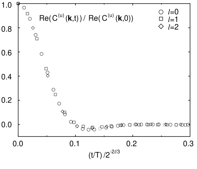
FIG. 12.: The real part of the autocorrelation function $C^{(u)}({\bf k},t)=\left<{\bf u}^{*}({\bf k},0)\cdot{\bf u}({\bf k},t)\right>$ normalized to its equal time value $C^{(u)}({\bf k},0)$ for the mode ${\bf k}=2^{\ell}(1,1,1)$ of the small cascade. Shown are the three top levels. The correlation function decays very quickly, reflecting the chaotic behavior of the velocity field. The time, given in units of $T=\left<E_{0}\right>/\epsilon$, is rescaled according to the classical prediction $\tau^{(u)}_{\ell}\sim 2^{-2\ell/3}$ for the decay time.

The abscissa is rescaled according to (42), which makes all three correlation functions fall atop of each other. So it seems that if corrections to (42) exist, they are so small that they need more sophisticated methods to be revealed.

Next, we look at the temporal correlations of the energy on the highest level, plotted in Fig. 13.

=0.4

FIG. 13.: The autocorrelation function $C^{(E)}_{0}(t)$ of the energy on the top level, normalized to its equal time value $C^{(E)}_{0}(0)$ for the small cascade. The energy de-correlates by more than a factor of 10 more slowly than a single velocity mode. The time is given in units of $T=\left<E_{0}\right>/\epsilon$.

Apart from differences in shape, the remarkable feature is that the typical decay time is more than 10 times as long as that of individual Fourier modes. The temporal correlation is apparently dominated by the long-time fluctuations of the energy already noted in Fig. 5. The rapid fluctuations representative of the individual Fourier modes appear to be completely uncorrelated. The physical reason is that many different modes within a shell contribute to these rapid fluctuations, which are de-correlated through many random “collisions”. Just like in a gas of particles, the complicated interaction between many modes tends to randomize the individual motions.

If the small-scale fluctuations were a true random walk, the energy would slowly diffuse to take arbitrary values. But eventually the tendency of the dynamics to restore equilibrium will drive the energy back to its mean value. This requires a coherent motion of many individual Fourier modes, whose correlations need some time to build up. Thus the long time scale in the motion of the energy. So far the same argument would apply for a cascade in equilibrium, in the absence of driving. This is shown in Fig. 14 for a cascade of 8 shells,

=0.4

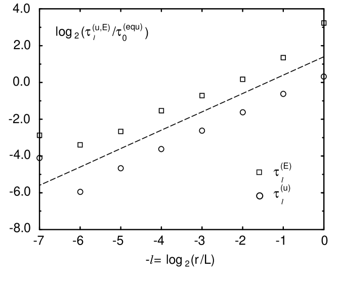
FIG. 14.: Correlations times $\tau^{(u,E)}_{\ell}$ for the small cascade in equilibrium, as a function of the level number. The dashed line corresponds to the theoretical prediction of (43). The time scale of the energy is longer than that of an individual mode by a factor of 4 on all levels.

which all perform fluctuations whose static distribution was shown in Fig. 6. Since the energies of all shells fluctuate around some common value $E_{av}$, and the local length scale is $2^{-\ell}L$, for dimensional reasons the time scale must be

$$\tau_{\ell}^{(equ)}\sim E_{av}^{-1/2}\;2^{-\ell}L\;.$$ (43)

The correlation times shown in Fig. 14 for both the energy and one of the velocity modes is calculated according to

$$\tau_{\ell}^{(E,u)}=\frac{\int_{0}^{\infty}C_{\ell}^{(E,u)}(t)\,dt}{C_{\ell}^{(E,u)}(0)}\quad,$$ (44)

and are found to corroborate the scaling law (43). As in the case of the top level of a Kolmogorov cascade, the correlation time of the energy is slower compared to an individual Fourier mode.

This changes fundamentally when looking at lower shells of a non-equilibrium cascade. For a turbulent cascade, one expects to recover the scaling (42), since the correlation of the energies are defined in terms of local quantities only. But remarkably, the scaling law (42) does not even approximately describe the scaling of $\tau^{(E)}_{\ell}$, which rather follows the power law

$$\tau^{(E)}_{\ell}\sim 2^{-\alpha\ell}\;,\alpha=0.094,$$ (45)

as seen in Fig. 15.

=0.4

FIG. 15.: Scaling of the correlation times $\tau_{\ell}^{(E)}$ of the energy correlation function $C^{(E)}_{\ell}(t)$ for the small cascade. The fit corresponds to $\tau^{(E)}_{\ell}\sim 2^{-0.094\ell}$, which is a very small decrease compared to the classical prediction of $\tau^{(E)}_{\ell}\sim 2^{-2\ell/3}$.

This means the time scale of the motion of the energy hardly gets shorter at small scales. The reason lies within the non-equilibrium properties of the cascade: Once a large fluctuation of the energy has built up on the highest level, it can only relax by being transported to a lower level. Thus the same long time dependence is imprinted on the lower level, which again can only be transferred to the next level. Thus on a given level, all time scales of the levels lying above appear, and apart form the single rescaling (45) the shape of the correlation function changes as well. This corresponds directly to the origin of intermittent fluctuations itself: fluctuations amplify because lower shells are driven by slowly varying energy input of the higher shells. Consequently fluctuations “ride” atop of the long-scale fluctuations and amplify. By looking at correlations between individual Fourier modes like (40) none of these long-range correlations are revealed. Correlations between the coherent structures of a turbulent velocity field will always be masked by the incoherent fluctuations of the individual modes.

It is interesting to note that in a numerical simulation of isotropic turbulence Yeung and Pope [22] have found very strong deviation from classical scaling as well. They looked at the Reynolds number dependence of the acceleration variance, which is a Lagrangian quantity. Like in our case, including fluctuations of the energy transfer according to Kolomogorov’s refined similarity hypothesis [3] cannot account for the corrections found. However, a meaningful definition of a Lagrangian quantity within our local approximation is difficult, since convection cannot be described properly. Therefore we do not know how to relate our findings with the results of Ref. [22] directly.

The second consequence of the extremely slow de-correlation of the energy is that the ratio of time scales of the energy and that of individual modes rapidly becomes larger on smaller scales. In the Langevin description the white noise term represents the irregular motion of individual Fourier modes, while our main interest lies with the large-scale fluctuations of the energy. In the scaling limit we are interested in the disparity between these scales becomes infinitely large. Thus a white-noise description should become better and better in the relevant limit.

VI Discussion

We have investigated mode-reduced approximations of the Navier-Stokes equation and found them to have anomalous scaling exponents in the inertial range. Intermittent fluctuations come about through rare excursions of the energy from its mean value, which originate from the top levels of the cascade. They are thus well described by a white-noise Langevin process, whose random forcing represents the motion of individual Fourier modes. The analytical solution shows [20] that such a Langevin cascade necessarily exhibits corrections to the classical scaling exponents. It is thus hard to see how any cascade with local coupling could avoid intermittency corrections in the inertial range, since for a chaotic motion there will always be fluctuations, and thus $D/R^{2}\neq 0$. In fact, as pointed out by Kraichnan [38], the only mechanism by which such fluctuations could be avoided is by sufficiently strong mixing in space, which in $k$-space would be represented by non-local interactions. The fact that our simple Langevin model gives an excellent description of a complicated network of Fourier modes is also highlighted by the excellent agreement in an equilibrium state. We have recently extended the comparison between the Langevin and the REWA model to the formation of singularities in the absence of viscosity [39]. In this case, which represents a state even farther from equilibrium than a Kolmogorov cascade, the two models still compare quantitatively. This allows for an analytical description of the singularities of the Euler equation [41] in the approximation of local coupling.

The second central point of our paper is to demonstrate that intermittency exponents can be calculated for a complex cascade with nonlinear, chaotic dynamics by analytical means. The only piece of information one needs about the turbulent flow concerns the local energy transfer. With this information, the global non-equilibrium properties determine the intermittency exponents, which is taken care of by the analytical calculation. In a very interesting paper, Olla [42] has recently carried out the same program directly from the Navier-Stokes equation. He assumes that the broadening of the distribution of the velocity field from a scale $r$ to $r/2$ is adequately described in a Gaussian approximation. Thus he is able to determine the analogue of the noise strength $R/D^{1/2}$ from perturbation theory. However, a major problem of Olla’s work is that he also does not deal adequately with the spatial structure of turbulence, but rather maps the problem on the same linear cascade structure we are considering here.

The most pressing problem remaining with the present mode representations is that the intermittency effects are quite small. Thus some important physical features are still missing. The most likely reason is the fact that a given eddy only feeds a single substructure, instead of branching out to several smaller structures overlapping with it in physical space. It has been shown [27, 19] that such a tree structure may strongly enhance intermittent fluctuations, owing to competition between different eddies on the same level. The procedures of the present paper can be directly carried over to this physical situation, as analytical solutions of the Langevin model with tree structure are available as well [40]. Unfortunately, there is no technique available which would link the Navier-Stokes equation to a cascade coupled locally in real and in $k$-space in a rational way. Since the value of intermittency exponents depends significantly on the properties of the local couplings [35], no quantitative prediction for real three-dimensional turbulence is possible using the more general tree structure.

An interesting fact revealed by our analysis is that the value of the correction exponents depends considerably on the mode selection. There is a tendency, observed earlier [18], for the size of fluctuations to decrease with the number of modes per shell. In [18], mode systems with up to 86 modes per shell have been considered, which also allow for more distant interactions between shells. Although it is interesting to look at the significance of more distant interactions, it does not remedy the fundamental problem of the present approximation, which is that the number of modes does not proliferate on small scales. In terms of interactions, there is still no competition between modes of the same scale. Thus no conclusions about the true intermittency exponents can be drawn from including more modes, as long as the spatial structure is not respected. In fact for a tree structure the number of localized boxes would increase like $2^{3\ell}$, each with a constant number of modes $N$. Comparing that with the total number of Fourier modes $(4\pi/3)(2^{3}-1)2^{3\ell}$ within a shell for three-dimensional turbulence, one obtains the estimate $N\approx 28$, which is close to the number $N=26$ of our small cascade [43]. Thus the small cascade already represents a physically reasonable choice for the number of locally interacting Fourier modes.

Finally we mention the so-called GOY model [44, 45], which contains only one complex mode per shell, and which has attracted considerable attention recently. Although it has no spatial structure, the intermittency exponents are comparable to those of real turbulence, which seems to contradict our above observations. We believe that the mechanisms at work are somewhat different here, since there exist pulses, which run down the cascade. These global coherent motions are much more effective in transporting fluctuations to smaller scales than in REWA cascades, where such structures are destroyed by intra-shell mixing. A separation of time scales between the total energy and the individual modes of a shell evidently does not exist. Another fact which points to global structures is the dependence of intermittency exponents on the form of viscous dissipation [45]. Still, this simple model remains interesting in particular in view of the analytical theory which has been developed for its inertial range properties [46], and which has a number of similarities with the one developed for the Langevin model [19, 20].

To conclude, we have investigated in detail how local coupling leads to intermittent fluctuations. In spite of many other interesting proposals, Landau’s and Kolmogorov’s original arguments remain among the most powerful for their understanding.

REFERENCES

- [1] A. N. Kolmogorov, “The local structure of turbulence in incompressible viscous fluid for very large Reynolds’ numbers”, C. R. Akad. Nauk SSSR 30, 301 (1941); “On degeneration of isotropic turbulence in an incompressible viscous fluid”, C. R. Akad. Nauk SSSR 31, 538 (1941); “Dissipation of energy in the locally isotropic turbulence”, C. R. Akad. Nauk SSSR 32, 16 (1941).
- [2] L. D. Landau and E. M. Lifshitz Fluid Mechanics, (Pergamon, Oxford, 1959; third edition, 1984).
- [3] A. N. Kolmogorov, “A refinement of previous hypotheses concerning the local structure of turbulence in a viscous incompressible fluid at high Reynolds number”, J. Fluid Mech. 13, 83 (1962).
- [4] A. M. Obukhov, “Some specific features of atmospheric turbulence”, J. Fluid Mech. 13, 77 (1962).
- [5] F. Anselmet, Y. Gagne, E. J. Hopfinger and R. Antonia, “High-order structure functions in turbulent shear flows”, J. Fluid Mech. 140, 63 (1984).
- [6] R. Benzi, S. Ciliberto, R. Tripiccione, C. Baudet, F. Massaioli and S. Succi, “Extended self-similarity in turbulent flows”, Phys. Rev. E 48, R29 (1993).
- [7] R. Benzi, S. Ciliberto, C. Baudet, G. R. Chavarria and R. Tripiccione, “Extended self-similarity in the dissipation range of fully developed turbulence”, Europhys. Lett. 24, 275 (1993).
- [8] J. Herweijer and W. van de Water, “Universal shape of scaling functions in turbulence”, Phys. Rev. Lett. 74, 4651 (1995).
- [9] B. Castaing, Y. Gagne and E. J. Hopfinger, “Velocity probability density functions of high Reynolds number turbulence”, Physica D 46, 177 (1990).
- [10] M. Nelkin, “What do we know about self-similarity in fluid turbulence?”,J. Stat. Phys. 54, 1 (1989).
- [11] S. Douady, Y. Couder, and M. E. Brachet, “Direct observation of the intermittency of intense vorticity filaments in turbulence”, Phys. Rev. Lett. 67, 983 (1991).
- [12] S. Kida and K. Ohkitany, “Spatio-temporal intermittency and instability of a forced turbulence”, Phys. Fluids A 4, 1018 (1992).
- [13] H. K. Moffatt, S. Kida, and K. Ohkitany, “Stretched vortices - the sinews of turbulence; large-Reynolds-number asymptotics”, J. Fluid Mech. 259, 241 (1994).
- [14] J. Jiménez, A. A. Wray, P. G. Saffman, and R. S. Rogallo, “ The structure of intense vorticity in inhomogeneous isotropic turbulence”, J. Fluid Mech. 255, 65 (1993).
- [15] Z.–S. She and E. Leveque, “Universal scaling laws in fully developed turbulence”, Phys. Rev. Lett. 72, 336 (1994).
- [16] V. L’vov and I. Procaccia, “Exact resummations in the theory of hydrodynamic turbulence. I. The ball of locality and normal scaling”, Phys. Rev. E 52, 3840 (1995); “II. A ladder to anomalous scaling”, Phys. Rev. E 52, 3858 (1995).
- [17] J. Eggers and S. Grossmann, “Does deterministic chaos imply intermittency in fully developed turbulence?”, Phys. Fluids A 3, 1958 (1991).
- [18] S. Grossmann and D. Lohse, “Scale resolved intermittency in turbulence”, Phys. Fluids 6, 611 (1994).
- [19] J. Eggers, “Intermittency in dynamical models of turbulence”, Phys. Rev. A 46, 1951 (1992).
- [20] J. Eggers, “Multifractal scaling from nonlinear turbulence dynamics: analytical methods”, Phys. Rev. E 50, 285 (1994).
- [21] J. A. Domaradzki and W. Liu, “Approximation of subgrid-scale energy transfer based on the dynamics of resolved scales of turbulence”, Phys. Fluids 7, 2025 (1995).
- [22] P. K. Yeung and S. B. Pope, “Lagrangian statistics from direct numerical simulations of isotropic turbulence”, J. Fluid Mech. 207, 531 (1989).
- [23] A. M. Obukhov, “Some general properties of equations describing the dynamics of the atmosphere”, Atmos. Ocean. Phys. 7, 471 (1971).
- [24] E. B. Gledzer, “Systems of hydrodynamic type admitting two quadratic integrals of motion”, Sov. Phys. Dokl. 18, 216 (1973).
- [25] M. Yamada and K. Ohkitami, “Lyapunov spectrum of a chaotic model of three-dimensional turbulence”, J. Phys. Soc. Jpn 56, 4210 (1987).
- [26] S. Grossmann and D. Lohse, “Intermittency exponents”, Europhys. Lett. 21, 201 (1993).
- [27] J. Eggers and S. Grossmann, “Anomalous turbulent velocity scaling from the Navier-Stokes equation”, Phys. Lett. A 156, 444 (1991).
- [28] M. Farge, “Wavelet transforms and their applications to turbulence”, Ann. Rev. Fluid Mech. 24, 395 (1992).
- [29] C. Meneveau, “Analysis of turbulence in the orthonormal wavelet representation”, J. Fluid Mech. 232, 469 (1991).
- [30] P. L. Garrido, J. L. Lebowitz, C. Maes, and H. Spohn, “Long-range correlations for conservative dynamics”, Physical Rev. A 42, 1954 (1990).
- [31] C. W. Gardiner, “Handbook of Stochastic Methods”, (Springer, Berlin, 1983).
- [32] R. H. Kraichnan, “Helical turbulence and absolute equilibrium”, J. Fluid Mech. 59, 745 (1973).
- [33] S. Orszag, “Lectures on the Statistical Theory of Turbulence” in: Fluid Dynamics 1973, Les Houches Summer School of Theoretical Physics, edited by R. Balian and J. L. Peube, (Gordon and Breach, 1977).
- [34] H. Tennekes and J. L. Lumley, A First Course in Turbulence, (MIT Press, 6th ed., 1980).
- [35] S. Grossmann and D. Lohse, “Intermittency in the Navier-Stokes dynamics”, Z. Phys. B 89, 11 (1992).
- [36] W. H. Press, S. A. Teukolsky, W. T. Vetterling, and B. P. Flannery, Numerical Recipes, (Cambridge University Press, 2nd edition, 1986).
- [37] R. M. Kerr and E. D. Siggia, “Cascade model of fully developed turbulence”, J. Stat. Phys. 19, 543 (1978).
- [38] R. H. Kraichnan, “On Kolmogorov’s inertial-range theories”, J. Fluid Mech. 62, 305 (1974).
- [39] C. Uhlig and J. Eggers, “Singularities in a cascade model of the Euler equation”, manuscript in preparation (1996).
- [40] C. Uhlig and J. Eggers, “A stochastic model of turbulence on a fractal tree”, unpublished manuscript (1994).
- [41] A. J. Majda, “Vorticity, turbulence, and acoustics in fluid flow”, SIAM Review 33, 349 (1990).
- [42] P. Olla, “A closure model for intermittency in three-dimensional incompressible turbulence”, Phys. Fluids 7, 1598 (1995).
- [43] E. D. Siggia, “Origin of intermittency in fully developed turbulence”, Phys. Rev. A 15, 1730 (1977).
- [44] M. H. Jensen, G. Paladin, and A. Vulpiani, “Intermittency in a cascade model for three-dimensional turbulence”, Phys. Rev. A 43, 798 (1991).
- [45] R. Benzi et al, “Scaling and dissipation in the GOY shell model”, Phys. Fluids 7, 617 (1995).
- [46] R. Benzi, L. Biferale, and G. Parisi, “On intermittency in a cascade model for turbulence”, Physica D 65, 163 (1993).