Exploring Periodic Orbit Expansions and Renormalisation
with the Quantum Triangular Billiard.

Abstract

A study of the quantum triangular billiard requires consideration of a boundary value problem for the Green’s function of the Laplacian on a trianglar domain. Our main result is a reformulation of this problem in terms of coupled non–singular integral equations. A non–singular formulation, via Fredholm’s theory, guarantees uniqueness and provides a mathematically firm foundation for both numerical and analytic studies. We compare and contrast our reformulation, based on the exact solution for the wedge, with the standard singular integral equations using numerical discretisation techniques. We consider in detail the (integrable) equilateral triangle and the Pythagorean 3-4-5 triangle. Our non–singular formulation produces results which are well behaved mathematically. In contrast, while resolving the eigenvalues very well, the standard approach displays various behaviours demonstrating the need for some sort of “renormalisation”. The non-singular formulation provides a mathematically firm basis for the generation and analysis of periodic orbit expansions. We discuss their convergence paying particular emphasis to the computational effort required in comparision with Einstein–Brillouin–Keller quantisation and the standard discretisation, which is analogous to the method of Bogomolny. We also discuss the generalisation of our technique to smooth, chaotic billiards.

1 Introduction

The main focus of this paper is on contemporary issues in quantum chaos. In particular the convergence problems of periodic orbit expansions, the computational effort needed in their generation, and their status as the generalisation of Einstein–Brillouin–Keller quantisation to classically chaotic systems. To begin we consider the place our problem has in a broader context.

1.1 The need for a semiclassical limit.

Many problems in mathematical physics reduce to the solution of boundary value problems for partial differential equations or infinite matrices: wave propagation, diffusion, lattice statistical mechanics, stochastic problems, thermodynamic formalism in classical mechanics, an so on. Often, the “observables” can be expressed in terms of the eigenvalues and eigenvectors of some operator. The spectral problem of operators is of wide interest in mathematics as well.

Unfortunately, these problems can only be solved in integrable cases, in which an $n$–degree of freedom problem reduces to $n$ 1–degree of freedom problems. By “solve” we mean an effective, efficient, mathematically well behaved means of calculation which affords an opportunity for intuitive understanding. The only way to proceed is to recognise that the problem has to be divided in two: the lower energy, long wavelength, portion of the spectrum and the high energy, short wavelength, portition of the spectrum. The former regime is approximately reduced to the diagonalisation of a finite matrix. In the latter regime one uses semiclassical approximations. The stategy then is to develop the two techniques sufficiently and piece together their results to obtain a global understanding of the spectrum.

For practical purposes the only global information one often needs is Weyl’s density of states. Other times one simply requires the ground and first few excited states. It is then important to know at what point the spectrum crosses over into the “semiclassical” regime. It appears that the semiclassical regime extends quite far down. In the case of the disk, using asymptotic approximations for the Bessel function, one finds that a semiclassical approach gives acceptable approximations even for the ground state. For special examples such as the equilateral triangle and other problems solved by “Bethe Ansatz” the semiclassical approach gives the exact answer. For cases where global, detailed, spectral information is needed semiclassical methods are indispensible.

1.2 Semiclassical techniques

For historical reasons much of the development of semiclassical techniques has been driven by practical issues in optics and quantum mechanics. Such motivations have lead to mathematical developments such as the WKB method. Most of our motivation will come from quantum mechanics but optics will play a role.

Semiclassical techniques have long had an important role in quantum mechanics. In the early days of the old quantum theory (and in fact in some contemporary problems) they provided the only quantisation technique. Failing to quantise more complicated systems, notably the helium atom, they were replaced by quantum mechanics. There, through the WKB method, they reappeared as approximation techniques in 1–dimensional or separable problems.

Multidimensional, non–integrable quantum problems are much more difficult and are usually treated with integral equations or diagonalisation in some basis. While providing theoretical results to compare with experiment, such methods are computationally intense and afford little opportunity for intuitive understanding. Semiclassical techniques were first widely applied to such problems in optics [1]. They have also been applied to quantum chemistry [2] and more general problems of partial differential equations [3].

1.3 Semiclassical quantisation.

Although it was not widely realised, prior to the late 60s semiclassical quantisation was restricted to classically integrable systems using Einstein–Brillouin–Keller (EBK) quantisation [4, 3, 5]. It was then that Gutzwiller [6] developed a method of semiclassical quantisation based on the calculation of the Green’s function via a Laplace transform of the time–dependent propagator (heat kernel). For the latter a semiclassical approximation could be derived via Feynman’s path integral regardless of the integrablity of the corresponding classical system. Gutzwiller used the resulting periodic orbit expansion to determine the spectrum of the Kepler problem, and later, an anisotropic version of it.

Around the same time, Balian and Bloch [7] obtained a similar result while extending a classical result of Weyl for the density of states of the Laplacian. They used a multiple expansion technique for the Green’s function due originally to Carlemann. Weyl’s formula is only relevant if one wishes to calculate certain sums over the spectrum. Balian and Bloch were interested in refining the Weyl result to incorporate the “shell structure” of the spectrum. They appear to have been motivated by certain spectral sums arising in nuclear physics.

In recent years, mostly driven by resurgent interest in classical chaos, there has been renewed interest in this work. The prime motivation has been to rehabilitate the old quantum theory by providing a quantization rule, analogous to EBK quantisation, for non-integrable systems. It is well known [4] that periodic orbit expansions are absolutely divergent for chaotic systems due to an exponential proliferation of periodic orbits. Despite this, they have had some empirical success as rules for “quantising chaos”. This motivatives the oft–stated hope that the series are conditionally convergent. The well–known properties of conditionally convergent series with regards rearrangment [8] then begs the question: In what order should the sum be carried out?

In an effort to overcome this difficulty, the original periodic orbit expansions have been refined in many ways. These refinements tend to be motivated from results in other areas of mathematics and physics: the theory of the Riemann zeta function, topology of hyperbolic flows in classical chaos, the boundary integral method for partial differential equations, and scattering theory. These refinements include: the Riemann–Siegel lookalike formula and pseudo–orbit expansions [9], cycle expansions [10], surface of section techniques [11] and inside–outside duality [12].

Some refinement of Weyl’s formulae in the calculation of spectral sums has been motivated from the Selberg trace formula for geodesic motion on hyperbolic manifolds [5, 13].

These techniques have been tested on a number of chaotic systems including: the hyperbola billiard [14], the helium atom [15], the wedge billiard in a gravitational field [16, 17], the Sinai billiard [18, 19], the 3 disk system [10, 20], and smooth Hamiltonian systems [21]. Much progress has been made, as can most readily be seen in [14] and [16] where various modifications are compared.

Despite the relative success of these improvements, they have all come from well motivated, but largely heuristic arguments and derivations. The well known mathematical difficulties are not directly tackled. An exception to this is some recent and very important work of Georgeot and Prange [22]. Starting with the integral equations of Balian and Bloch they apply the Fredholm theory of integral equations [23] to show, amongst other things, that the pseudo–orbit expansions for smooth billiards converge. The proper order of summation, of what is clearly a conditionally convergent series, is dictated by the Fredholm theory. Thus, at least for smooth billiards, it seems that the long standing questions regarding convergence have been settled. (well, maybe. See section 7.2.)

Apart from convergence issues, there is the equally serious question of computational effort. It is fairly clear from the literature that, unlike EBK quantisation, periodic orbit expansions become more and more computationally intensive as one seeks higher and higher eigenvalues. Furthermore this remains the case even with refinements which improve convergence [24]. While it is clear that exponential proliferation is the cause, it contradicts the correspondance principle which suggests that the semiclassical approximation should improve with “larger quantum numbers”. It may be, however, that this expectation is intertwined with our “integrable” intuition and needs to be reassessed in these “chaotic” times.

Thus, despite the progress made, mystery continues to surround semiclassical quantisation of non–integrable systems.

1.4 A role for the triangular billiard

Our aim is to critically examine of the nature of semiclassical quantisation rules. To do this we seek out a model problem which is sufficiently simple to enable a first principles derivation which maintains reasonable standards of mathematical rigour. Whereas we do not seek, and are not capable of, a rigorous derivation, we aim at one which can plausibly form the basis for a rigorous approach. Our choice is the quantum triangular billiard.

The quantum triangular billiard is well suited to a first-principles derivation. Being a billiard, the boundary value problem for the Green’s function can be converted to an integral equation. This permits the application of a substantial body of standard theory. As with Georgeot and Prange, our main tool will be the Fredholm theory of integral equations. Most importantly, piecewise linear boundaries afford us much needed flexibility. Our discussion is immediately applicable to polygonal billiards. Although our notation will have an eye toward this generalisation, we will limit ourselves to triangles so as not be be distracted from our aim. The prospects for handling more general billiards, in particular those whose boundaries have smooth components, will be discussed in Section 7.2.

The quantum triangular billiard has been studied in a number of contexts. In the context of quantum chaology it has not attracted much attention because polygonal billards are not chaotic [25] (see however [26]) so that one does not have exponential proliferation of periodic orbits. Despite this, it is still (generically) a non-integrable system, intermediate between integrable systems and chaotic ones, and so still of interest in its own right. It has also been considered in the contexts of eigenvalue degeneracies [27], energy level statistics [28], and modifications of periodic orbit expansions due to non-isolated and diffractive periodic orbits [29]. Integrable triangles have eigenfunctions which are exactly expressed in terms of a finite superposition of plane waves via the Bethe Ansatz [30]. The general triangle has also been studied in an effort to extend the Bethe ansatz [31]. The Weyl formula for polygonal billiards has long been known [32]. More recently this result has been extended to calculate determinant of the Laplacian [33].

1.5 Statement of problem

To be more precise, the task we have set ourselves is the calculation of the spectrum of the Dirichlet Laplacian on a triangular domain. All spectral information conveniently resides in the Green’s function which is the unique solution of the boundary value problem

$$\nabla^{2}T(\boldsymbol{x},\boldsymbol{x}_{i})+z\,T(\boldsymbol{x},\boldsymbol{x}_{i})=0,\quad\mathbf{x}\in\triangle/\{\mathbf{x}_{i}\}$$ (1.1a)

$$\lim_{\epsilon\to 0}\oint_{C_{\mathbf{x}_{i}}}\nabla T(\boldsymbol{x},\boldsymbol{x}_{i})\,.\,d\/\boldsymbol{n}=1$$ (1.1b)

$$T(\boldsymbol{x},\boldsymbol{x}_{i})=0\quad\text{ for }\mathbf{x}\in\partial\triangle$$ (1.1c)

$C_{\mathbf{x}_{i}}$ is a circular contour of radius $\epsilon$ taken counterclockwise around the “source” point, $\mathbf{x}_{i}$. $\triangle$ denotes the triangular domain and $\partial\triangle$ denotes its boundary.

The unit source condition, (1.1b), is usually specified as a Dirac $\delta$–function inhomogeneity in (1.1a). We take the opportunity to remind the reader of this more precise description, even if it is somewhat old fashioned [34].

We are now in a position to be precise about the semiclassical limit. In this problem there are two natural length scales: the “de Broglie” wavelength $1/\sqrt{z}$ and any length $L$ whose order of magnitude reflects the geometric distances over which the domain varies. For $\triangle$ it is the length of the sides. More complicated domains may provide other length scales which may or may not be a similar order of magnitude. The semiclassical limit is where the “extent” of the triangle is much larger than the “de Broglie” wavelength, $\sqrt{z}L\gg 1$. Cast in this mathematical language, the semiclassical limit becomes a problem of asymptotic analysis.

1.6 Standard integral equation approach

For generic triangles the classical problem is non–integrable so that EBK is not applicable. The only way to obtain further analytic insight is to convert the boundary value problem into an integral equation using Greens’ theorem. This is a standard technique in mathematical physics with a long history. It is widely used in electrostatics [34], diffraction [35], and quantum scattering theory [36], both as a way to derive integral equations and also as a starting point for analytic and numerical approximations. It’s (indirect) use in the study of quantum billiards began with Balian and Bloch [7]. We shall refer to this technique as the “standard approach” or the “free–based method”.

For the Helmholtz equation various types of integral equations can be obtained. For the eigenfunctions one obtains an homogenous integral equation of the second kind. For the Greens’ function one obtains an inhomogenous integral equation the second kind. Whilst there is a close connection between the two, the Fredholm theory gives the results needed to generate periodic orbit expansions only in the inhomogenous case. One is thus forced to study the spectral problem via the Green’s Function.

It is well known [37] (though sometimes overlooked) that in contrast with smooth billiards, the standard integral equations for polygonal billiards are singular. By this we mean that the requirements on the kernel demanded by Fredholm theory are not satisfied. Singular integral equations are known to be pathological. For example, the Lippmann–Schwinger equations for the quantum three body problem, which are singular, do not have unique solutions [36]. In the literature on the Helmholtz equation, singular equations are known to yield “spurious solutions” [27, 37]. Although useful information can be extracted from these equations, the presence of pathologies creates the need for ad–hoc techniques, caution, and ultimately, doubt.

The main result of this paper is the derivation of non–singular integral equations for the Green’s function of the quantum triangular billiard. The derivation of non–singular integral equations from singular ones has a precedent in the work of Faddeev on the quantum three body problem [36]. The basic idea of Faddeev’s work is that it is neccessary to treat part of the interaction in an explicit non–perturbative manner. Faddeev does this by eliminating the potential in favour of the T–matrix. As we will discuss in Section 2.8 a direct application of Faddeev’s technique is not convenient for our problem. Instead we follow the spirit by basing a derivation on the Green’s function for the wedge.

Whereas most treatments of the quantum billiard problem depict the derivation of the integral equations as straightforward and concentrate on the generation of periodic orbit expansions, we shall show that for polygonal billiards this is not the case. Although we shall present a relatively compact and well motivated derivation, this does not reflect the tortuous path we took to reach it.

1.7 Outline of paper

We begin in Section 2 with an outline of the standard approach, presenting more detail than is customary in order to demonstrate some subtleties which are usually overlooked. The derivation will be accompanied by an elaboration of the relatively well known intepretation in terms of a “quantum Poincaré section”. We then demonstrate the singular nature of the standard integral equations and discuss ways in which they can be manipulated to obtain non–singular equations. We also emphasise the perturbative nature of the whole Green’s theorem–based approach. We then warm up for the wedge–based approach by rederiving the standard integral equations from a perturbation about the half–plane Green’s function. A similar derivation has recently been presented by Li and Robnik [39].

In Section 3 we outline the derivation of non–singular integral equations based on the exact solution for the wedge Green’s function. The implementation of the non–singular formulation requires a detailed analytic and computational understanding of this solution. In Section 4 we give the necessary technical detail for the wedge–based kernel. In the appendix we give an outline of the derivation of the wedge Green’s function. In Section 5 we present and compare, for purposes of validation, the results obtained from a standard numerical treatment of both the singular and non–singular integral equations. In particular we present the eigenvalues for the equilateral and Pythagorean 3-4-5 triangles by examining the zeros of the Fredholm determinant. We show that the Fredholm determinant for the discretised singular equation does not converge although it resolves the eigenvalues well. In contrast, the non–singular equation behaves well, as the Fredholm theory demands.

Given a suitable integral equation, the derivation of periodic orbit expansions is more or less mapped out by Georgeot and Prange. Let us briefly outline their discussion. The Fredholm theory expresses the solution of an integral equation in terms of a resolvent kernel $H_{\lambda}$ and a Fredholm determinant $\Delta(\lambda)$ in the form

$$x(t)=x_{0}(t)+\frac{1}{\Delta(\lambda)}\int_{a}^{b}H_{\lambda}(t,s)x_{0}(s)\,ds$$ (1.2)

[23]. The eigenvalues are then the zeros of the Fredholm determinant, which one identifies as a zeta function. The Fredholm determinant can be expanded in series using the identity $\log\det(I-K)=\operatorname{Tr}\log(1-K)$ [38]. The expansion of $\log(I-K)$ in powers of $K$ has a finite radius of convergence. However exponentiating the series and re–expanding gives the standard Fredholm series which has an infinite radius of convergence [23, Theorem 6.5.2]. A semiclassical expansion of the traces $\operatorname{Tr}(K^{n})$, which appear in this series, then provides a convergent periodic orbit expansion for this zeta function which one identifies with the psuedo–orbit expansion.

At this point it is necessary to make a terminological aside. The term “periodic orbit expansion” can refer to the original Gutzwiller series or any of its refinements. The context of discussion allows one to use it without qualification. However, in order to emphasise the firm foundation provided by the Fredholm theory, we feel that it is perhaps appropriate to occasionally use the term “semiclassical Fredholm series”.

In Section 6 we use the Fredholm theory to analyse the convergence of resulting periodic orbit expansion. Here it will become clear that while Fredholm theory solves the convergence problem the number of terms needed for convergence grows like $\sqrt{E}$. The semiclassical approximation of the $n$–th term in the series expansion of the Fredholm determinant requires all $n$–bounce periodic orbits. For the triangle the number of such orbits grows polynomially in n. The computation effort in the periodic orbit expansion is then polynomial in $\sqrt{E}$. In contrast the effort for chaotic systems is exponential. We compare this effort with the $O(n^{3})$ effort needed in the numerical discretisation of the integral equations. This comparision clearly defines how far we are from the goal of emulating EBK quantisation for chaotic systems.

We conclude with a discussion in Section 7. Here we present the singular equation as a simple model system which requires “renormalisation”. We note the presence of logarithmic singularities in the Fredholm series making it comparable to perturbation series in quantum field theory. The wedge based theory is then interpreted as a first principles, mathematically firm, “renormalisation scheme” where any ad–hoc“regularisation” and “subtraction of infinities” is absent. We then present arguments that cast doubt on the validity of the Balian–Bloch integral equations for smooth billiards. We then suggest ways in which our construction can be carried over in principle to smooth billiards. We also discuss the relationship between the Fredholm series approach and other modifications of Gutzwiller’s original trace formula. We also present our construction as a way to derive, in a mathematically satisfactory way, Keller’s geometrical theory of diffraction [1].

2 Standard Approach: Singular Integral Equations

2.1 Standard pre–integral equation

The standard approach is based on the free Greens function. This is the solution of the Helmholtz equation on the Euclidean plane which decreases at infinity and has a unit source.

$$G_{0}(\boldsymbol{x},\boldsymbol{x}_{f})=-\frac{i}{4}H_{0}^{(1)}(\sqrt{z}|\boldsymbol{x}-\boldsymbol{x}_{f}|)$$ (2.1)

where $H_{0}^{(1)}(z)$ is the zeroth order Hankel function of the first kind [40].

Our main point is that this is a choice and that for polygonal billiards it is a poor choice. Let us thus begin with any Greens’ function, i.e. any function $F(\boldsymbol{x},\boldsymbol{x}_{f})$ which is a solution of the Helmholtz equation with a unit source. The domain on which $F(\boldsymbol{x},\boldsymbol{x}_{f})$ is defined and the boundary conditions it satisfies are totally arbitrary.

\psfrag{P0}{\Large$\boldsymbol{P}_{0}$}\psfrag{P1}{\Large$\boldsymbol{P}_{1}$}\psfrag{P2}{\Large$\boldsymbol{P}_{2}$}\psfrag{r0}{$\mathbf{r}_{0}(t)$}\psfrag{r1}{$\mathbf{r}_{1}(t)$}\psfrag{r2}{$\mathbf{r}_{2}(t)$}\psfrag{n0}{$\mathbf{n}_{0}$}\psfrag{n1}{$\mathbf{n}_{1}$}\psfrag{n2}{$\mathbf{n}_{2}$}\psfrag{xi}{$\mathbf{x}_{i}$}\psfrag{xf}{$\mathbf{x}_{f}$}\psfrag{x(s)}{$\mathbf{x}(s)$}\psfrag{t}{$t$}\psfrag{d}{$\delta$}\includegraphics[height=188.62654pt]{intPath.eps}

Figure 1: Contour for derivation of pre–integral equation. For convenience distances $t$ are defined with respect the nearest vertex in a counterclockwise sense. The heads of vectors are denoted using points. The integration region $D$ is shaded and the sense of $\partial D$ is shown.

Applying Green’s second identity,

$$\int_{D}(\phi\nabla^{2}\psi-\psi\nabla^{2}\phi)\,dx\,dy=\int_{\partial D}(\phi\nabla\psi-\psi\nabla\phi)\,.\,d\/\boldsymbol{n},$$ (2.2)

with $\phi=T(\boldsymbol{x},\boldsymbol{x}_{i})$ and $\psi=F(\boldsymbol{x},\boldsymbol{x}_{f})$ to the domain $D$ given in Figure 1, taking the width of the channels $\delta$ to zero, and using continuity in the usual way, one obtains

$$\left(\int_{\partial\triangle}-\int_{C_{{\boldsymbol{x}_{i}}}}-\int_{C_{{\boldsymbol{x}_{f}}}}\right)[T(\boldsymbol{x},\boldsymbol{x}_{i})\nabla F(\boldsymbol{x},\boldsymbol{x}_{f})-F(\boldsymbol{x},\boldsymbol{x}_{f})\nabla T(\boldsymbol{x},\boldsymbol{x}_{i})]\,.\,d\/\boldsymbol{n}=0.$$ (2.3)

$C_{\boldsymbol{x}_{i}}$ and $C_{\boldsymbol{x}_{f}}$ are circular contours of radius $\epsilon$.

In the integral over $C_{\boldsymbol{x}_{i}}$ all functions, except $\nabla T$, are continuous and can be approximated to $O(\epsilon)$ by their values at $\boldsymbol{x}_{i}$. Using this, the unit source condition, and taking $\epsilon\to 0$ we obtain

$$\begin{split}\lim_{\epsilon\to 0}\oint_{C_{\boldsymbol{x}_{i}}}&\left[T(\boldsymbol{x},\boldsymbol{x}_{i})\nabla F(\boldsymbol{x},\boldsymbol{x}_{f})-F(\boldsymbol{x},\boldsymbol{x}_{f})\nabla T(\boldsymbol{x},\boldsymbol{x}_{i})\right]\,.\,d\/\boldsymbol{n}\\ &=-F(\boldsymbol{x}_{i},\boldsymbol{x}_{f})\left[\lim_{\epsilon\to 0}\int_{C_{\boldsymbol{x}_{i}}}\nabla T(\boldsymbol{x},\boldsymbol{x}_{i})\,.\,d\/\boldsymbol{n}\right]\\ &=-F(\boldsymbol{x}_{i},\boldsymbol{x}_{f})\end{split}$$ (2.4)

The integral over $C_{\boldsymbol{x}_{f}}$ is evaluated similarly.

Using the Dirchlet boundary condition satisfied by $T(\boldsymbol{x},\boldsymbol{x}_{i})$ we finally obtain

$$\mathrm{T}(\boldsymbol{x_{f}},\boldsymbol{x_{i}})=\mathrm{F}(\boldsymbol{x_{i}},\boldsymbol{x_{f}})-\int_{\partial\triangle}F(\boldsymbol{x},\boldsymbol{x}_{f})\nabla T(\boldsymbol{x},\boldsymbol{x}_{i})\,.\,d\/\boldsymbol{n}$$ (2.5)

The integration in (2.5) is concentrated on the boundary of the domain but also involves values of the unknown function at arbitrary points in the interior. Interpreted as an integral equation on $\triangle$ it has a very singular kernel. The standard approach instead regards this as an equation which determines the solution in the interior given it’s normal gradient on the boundary. For this reason we refer to (2.5) as the pre–integral equation. Let us pause for a moment to interpret this equation.

2.2 Poincaré section interpretation

The boundary of the domain in (2.5) plays a distiguished role very similar to its role in the classical problem. In the classical problem Birkhoff defined a Poincaré section for billiards consisting of pairs $(q,p)$ giving the position and tangential momentum at each collision with the boundary. A particular classical orbit is then represented in the Poincaré section by a sequence of points, $(q_{n},p_{n}),n=0,1,2\ldots,\infty$. Knowing that the motion between collisions is free we can explicitly give the full orbit from this sequence. For billiards the first return map, $q_{n+1}=f(q_{n},p_{n}),p_{n+1}=g(q_{n},p_{n})$, be obtained explicitly. This “surface of section” construction then reduces the problem to a simpler dynamics, that of a map, on a space of reduced dimensionality.

This construction is identical in spirit to the above interpretation of the pre–integral equation. Rather than consider the space of all functions defined on $\triangle$ as dynamical variables we have reduced the dimensionality of the unknowns to the space of functions on $\partial\triangle$. All we need an integral equation on this space to play the role of a “quantum first return map” and whose unique solution is the actual boundary normal derivative.

This analogy is of course not direct because of the fundamental differences between classical and quantum mechanics. In quantum mechanics there is no sensible concept of “phase space”. The state of the system, in the Schroedinger form of quantum mechanics, involves only the interior and boundary configuration coordinates. Furthermore $q$ is the independent variable of the wave function rather than a dynamical variable $q(t)$.

It would appear that a “quantum first return map” can be obtained in a straightforward manner by taking the gradient of (2.5) with respect to $\boldsymbol{x}_{f}$, evaluating the limit as $\boldsymbol{x}_{f}$ tends to the boundary and projecting out the normal derivative. We shall refer to this process as the boundary limit.

2.3 The boundary limit

The boundary limit is in fact rather subtle. Let us now take up the standard approach in which the free Green’s function is chosen for $F(\boldsymbol{x},\boldsymbol{x}_{f})$.

At this point it is necessary to introduce some notation. Refering to Figure 2 we locate the verticies of the triangle at $\boldsymbol{P}_{0},\boldsymbol{P}_{1}$ and $\boldsymbol{P}_{2}$. The sides of the triangle are labelled with the integers $0,1,2$ so that $\partial\triangle=0+1+2$. The length of side $\mu$ is $l_{\mu}$.

\psfrag{0}{$0$}\psfrag{1}{$1$}\psfrag{2}{$2$}\psfrag{P0}{\Large$\boldsymbol{P}_{0}$}\psfrag{P1}{\Large$\boldsymbol{P}_{1}$}\psfrag{P2}{\Large$\boldsymbol{P}_{2}$}\psfrag{l0}{$l_{0}$}\psfrag{l1}{$l_{1}$}\psfrag{l2}{$l_{2}$}\psfrag{phi0}{$\phi_{0}$}\psfrag{phi1}{$\phi_{1}$}\psfrag{phi2}{$\phi_{2}$}\includegraphics[height=188.62654pt]{FreeNotation.eps}

Figure 2: Notation: Free–based integral equation

For convenience we parameterise each segment of the boundary using the distance from the vertex immediately clockwise:

$$\boldsymbol{r}_{0}(s) =\boldsymbol{P}_{0}+\frac{\boldsymbol{P}_{1}-\boldsymbol{P}_{0}}{|\boldsymbol{P}_{1}-\boldsymbol{P}_{0}|}\,s\quad\quad 0\leq s\leq l_{0}$$ (2.6a)

$$\boldsymbol{r}_{1}(s) =\boldsymbol{P}_{1}+\frac{\boldsymbol{P}_{2}-\boldsymbol{P}_{1}}{|\boldsymbol{P}_{2}-\boldsymbol{P}_{1}|}\,s\quad\quad 0\leq s\leq l_{1}$$ (2.6b)

$$\boldsymbol{r}_{2}(s) =\boldsymbol{P}_{2}+\frac{\boldsymbol{P}_{0}-\boldsymbol{P}_{2}}{|\boldsymbol{P}_{0}-\boldsymbol{P}_{2}|}\,s\quad\quad 0\leq s\leq l_{2}$$ (2.6c)

Then we define

$$X_{\mu}(t) =\nabla T(\boldsymbol{r}_{\mu}(t),\boldsymbol{x}_{i})\,.\,\boldsymbol{n}_{\mu} 0<t<l_{\mu}$$ (2.7a)

$$X^{0}_{\mu}(t) =2\nabla G_{0}(\boldsymbol{r}_{\mu}(t),\boldsymbol{x}_{i})\,.\,\boldsymbol{n}_{\mu} 0<t<l_{\mu}$$ (2.7b)

$$K_{\mu\nu}(t,s) =-2\nabla G_{0}(\boldsymbol{r}_{\nu}(s),\boldsymbol{r}_{\mu}(t))\,.\,\boldsymbol{n}_{\mu} 0<t<l_{\mu}\,,\quad 0<s<l_{\nu}$$ (2.7c)

where $\mu=0,1,2$, $\nu=0,1,2$. The need for the mysterious factors of 2 will soon be divined.

Formally taking the boundary limit towards side $0$, we obtain

$$\begin{split}2X_{0}(t)&=X^{0}_{0}(t)+\int_{0}^{l_{0}}K_{00}(t,s)X_{0}(s)\,ds\\ &\quad\quad+\int_{0}^{l_{1}}K_{01}(t,s)X_{1}(s)\,ds+\int_{0}^{l_{2}}K_{02}(t,s)X_{2}(s)\,ds\end{split}$$ (2.8)

In order to examine the boundary limit in detail we first present a diagramatic notation for (2.8) using the “Feynman rules” in Figure 3. Diagrammatic notation is totally equivalent to the algebraic notation and provides a convenient tool for generating perturbation expansions. In the present context it clearly elaborates the structure of the integral equations. It will also prove very useful and natural in the generation of periodic orbit expansions.

\psfrag{t}{$t$}\psfrag{s}{$s$}\psfrag{i}{$\mu$}\psfrag{j}{$\nu$}\psfrag{X}{$X_{\mu}(t)$}\psfrag{X0}{$X_{\mu}^{0}(t)$}\psfrag{K}{$K_{\mu\nu}(t,s)$}\includegraphics{FeynRules.eps}

Figure 3: Feynman Rules for translating between integral equations and diagrammatic representations. The arrows give the “flow” from $\mathbf{x}_{i}$ to $\mathbf{x}_{f}$ in the integral equations. They are needed to distinguish between $K_{\mu\nu}(t,s)$ and $K_{\nu\mu}(t,s)$.

The translation between notations is given by the usual rules

• Associate each factor in the integrand with an edge as given in Figure 3.

• The configuration space dimensions in the arguments of the integrand functions can be labelled on the triangle as shown. However these are fairly obvious and usually omitted.

• An integration along a side is associated with each vertex where two edges meet.

In Figure 4 we give a graphical representation of (2.8). The application of the Feynman rules is shown for part of the equation.

\psfrag{t}{$t$}\psfrag{s}{$s$}\psfrag{2}{$2$}\psfrag{e}{$=$}\psfrag{p}{$+$}\psfrag{IK}[l][l]{$\overbrace{\int_{0}^{d_{1}}ds}\underbrace{K_{01}(t,s)}\overbrace{X_{1}(s)}$}\includegraphics{intEqn.eps}

Figure 4: Graphical representation integral equation in naive boundary limit. Also shown is an example of the application of the Feynman rules.

At this stage we require the explicit form of the integral kernel

$$K_{\mu\nu}(t,s)=-\frac{i\sqrt{z}}{2}H_{1}^{(1)}(\sqrt{z}|\boldsymbol{\Delta}_{\mu\nu}(t,s)|)\frac{\boldsymbol{\Delta}_{\mu\nu}(t,s)\cdot\boldsymbol{n}_{\mu}}{|\boldsymbol{\Delta}_{\mu\nu}(t,s)|}$$ (2.9)

Here $\boldsymbol{\Delta}_{\mu\nu}(t,s)=\boldsymbol{r}_{\mu}(t)-\boldsymbol{r}_{\nu}(s)$ and $H_{1}^{(1)}(z)$ is a first order Hankel function of the first kind [40].

The subtlety in the boundary limit arises because

$$K_{\mu\nu}(t,s)\approx-\frac{1}{\pi}\frac{\boldsymbol{\Delta}_{\mu\nu}(t,s)\,.\,\boldsymbol{n}_{\mu}}{|\boldsymbol{\Delta}_{\mu\nu}(t,s)|^{2}}\quad|\boldsymbol{\Delta}_{\mu\nu}(t,s)|\ll\frac{1}{\sqrt{z}}$$ (2.10)

Apart from this the kernel is well behaved. The singularity occurs when $|\boldsymbol{\Delta}_{\mu\nu}(t,s)|$ is much smaller than the de Broglie wavelength so that it appears in the quantum regime. This distance is explicitly represented in the diagrammatic notation by the length of the segment corresponding to the “free propagator”, $K_{\mu\nu}$. It is thus easy to see when a singularity is encountered in the integration.

Let us now go back and do the boundary limit towards side $0$ in a more careful manner. In boundary limit we take $\boldsymbol{x}_{f}\to\boldsymbol{r}_{0}(t)$. Let us make the limit explicit by letting $\boldsymbol{x}_{f}=\boldsymbol{r}_{0}(t)-\epsilon\,\boldsymbol{n}_{0}$. We can readily “deform” our diagrammatic notation to accomodate this. In particular, in Figure 4 we can denote this deformation by simply displacing the final point slightly above the boundary.

It is easy to see that the boundary limits of the left hand side and the inhomogenous term exist by continuity, since $\boldsymbol{x}_{i}$ is strictly in the interior. It is also clear that, provided we stay away from the corners to keep the distance of free propagation bounded from below, the integrations over boundaries $1$ and $2$ have uniformly bounded integrands. They are then uniformly convergent and the boundary limit can be taken inside the integrals to give the formal result. The same is not true for the integration over boundary $0$. Here it is clear that the integrand develops a singularity in the boundary limit due to the presence of arbitrarily short distance propagation. The consequent lack of uniform convergence means that the formal boundary limit is not correct. This observation has already been made by Li and Robnik [39]. Their remedy is to perturb about the half–plane. Their treatment fits into our general scheme and we shall describe it in Section 2.7.

The boundary limit towards side $0$ can still be done, but care is required. In explicit form, we need to calculate.

$$\lim_{\epsilon\to 0}\int_{0}^{l_{0}}\frac{i\sqrt{z}}{4}H_{1}^{(1)}(\sqrt{z}\sqrt{(t-s)^{2}+\epsilon^{2}})\frac{\epsilon}{\sqrt{(t-s)^{2}+\epsilon^{2}}}X_{0}(s)\,ds$$ (2.11)

The integrand tends to zero as $\epsilon\to 0$ for $t\neq s$. Because the singularity in (2.10) reflects the unit source condition satisfied by the free Green’s function we expect to see $\delta$–function behaviour. This can be revealed explicitly by scaling the dummy variable according to $s=t+\epsilon x$ to obtain

$$\lim_{\epsilon\to 0}\int_{-t/\epsilon}^{(l_{0}-t)/\epsilon}\frac{i\sqrt{z}}{4}H_{1}^{(1)}(\sqrt{z}\epsilon\sqrt{x^{2}+1})\frac{1}{\sqrt{x^{2}+1}}X_{0}(t+\epsilon x)\,\epsilon\,dx$$ (2.12)

Expanding $X_{0}(t+\epsilon x)$ as a Taylor series in $\epsilon$ and using the small argument form for the Bessel function we can explicitly evaluate the integral for small $\epsilon$ to obtain

$$\left[\lim_{\epsilon\to 0}\frac{1}{2\pi}\int_{-t/\epsilon}^{(l_{0}-t)/\epsilon}\left\{\frac{1}{x^{2}+1}+O(\epsilon\log\epsilon)\right\}\,dx\right]X_{0}(t)=\frac{1}{2}X_{0}(t)$$ (2.13)

We see then that in the boundary limit the integrand behaves as $\frac{1}{2}\delta(x)$.

Repeating the calculation for the boundary limit toward sides $1$ and $2$ (or using a cyclic permutation of labels), we obtain

$$X_{0}(t) =X^{0}_{0}(t)+\int_{0}^{l_{1}}K_{01}(t,s)X_{1}(s)\,ds+\int_{0}^{l_{2}}K_{02}(t,s)X_{2}(s)\,ds$$ (2.14a)

$$X_{1}(t) =X^{0}_{1}(t)+\int_{0}^{l_{0}}K_{10}(t,s)X_{0}(s)\,ds+\int_{0}^{l_{2}}K_{12}(t,s)X_{2}(s)\,ds$$ (2.14b)

$$X_{2}(t) =X^{0}_{2}(t)+\int_{0}^{l_{0}}K_{20}(t,s)X_{0}(s)\,ds+\int_{0}^{l_{1}}K_{21}(t,s)X_{1}(s)\,ds$$ (2.14c)

This is a coupled form of the standard integral equation.

From (2.9) we observe that $K_{00}(t,s)=0$ because $\boldsymbol{r}_{0}(t)-\boldsymbol{r}_{0}(s)\perp\boldsymbol{n}_{0}$. It would be quite easy, in a first treatment, to ignore the fact that this is strictly only true for $t\neq s$ and use it in the formal boundary limit. This would lead to the same set of integral equations, except that the factors of 2 in (2.7) would be absent. We made this mistake in our early investigations and are quite confident that in doing so we have tread a well worn path.

2.4 Other treatments of the boundary limit

Balian and Bloch [7][I] derived the standard integral equations using potential theory. Their pre–integral equation (II.10) with (II.12) is of a different form to ours due to the choice of a double layer potential. We cannot understand how such an object can be obtained from Green’s theorem. The multiple scattering series which they give is nevertheless identical to the one obtained by iterating our equations. Potential theory is essentially the application of Green’s theorem to electrostatics. Because the Poisson equation is very different to the Helmholtz equation we feel that, while potential theory may give correct results, the delicacy of the problem demands the direct use of Green’s theorem.

Other authors [14, 27] derive the standard integral equations from the Helmholtz form of Greens’ second identity.

$$\int_{\partial D}ds^{\prime}\left\{\psi(\boldsymbol{r}^{\prime})\,\boldsymbol{n^{\prime}}\,.\,\nabla_{\boldsymbol{r}^{\prime}}G_{0}(\boldsymbol{r},\boldsymbol{r}^{\prime})-G_{0}(\boldsymbol{r},\boldsymbol{r}^{\prime})\,\boldsymbol{n^{\prime}}\,.\,\nabla_{\boldsymbol{r}^{\prime}}\psi(\boldsymbol{r}^{\prime})\right\}=\begin{cases}\psi(\boldsymbol{r})&\boldsymbol{r}\in D/\partial D\\ \frac{1}{2}\psi(\boldsymbol{r})&\boldsymbol{r}\in\partial D\\ 0&\boldsymbol{r}\not\in D\end{cases}$$ (2.15)

The mysterious factor of $\frac{1}{2}$ can be understood as being due to the indentation of the contour with a semicircle when $\boldsymbol{r}$ appears on the boundary.

The derivation proceeds by differentating (2.15). As our discussion shows, there is clearly some sort of boundary layer behaviour so that (2.15) needs to be supplemented with a statement of this behaviour. We suspect that performing the differentiation within the boundary layer is justified. As such we feel that Li and Robnik [39] are not strictly correct in describing the approach as in error. As the reader now has our discussion of the boundary limit, as well as the approach or Li and Robnik, we feel no particular need to elaborate any further.

Our study the boundary limit was motivated by the hope, forlorn as it turned out, that by doing the problem “carefully” the singular nature of the integral equations could be removed.

2.5 Singular nature: Fredholm theory

In taking the boundary limit it is convenient to use a notation which identifies each side of the triangle explicitly. This coupled form is convenient practical calculations because it provides a symbolic dynamics for quantum progagation. In the semiclassical analysis this will reduce to the natural symbolic dynamics for the classical propagation.

For theoretical purposes, in particular to apply the Fredholm theory, it is convenient to convert these coupled integral equations into a single integral equation. To do this we first define the cumulative arc length to each vertex from $\boldsymbol{P}_{0}$: $\sigma_{0}=0,\sigma_{\mu+1}=\sigma_{\mu}+l_{\mu}$, $\mu=1,2,3$. We can then define $\boldsymbol{x}(\sigma)=\boldsymbol{r}_{\mu}(\sigma-\sigma_{\mu})$ and $\boldsymbol{n}(\sigma)=\boldsymbol{n}_{\mu}$ for $\sigma_{\mu}<\sigma<\sigma_{\mu+1}$ giving the position and normal vectors in the Birkhoff co–ordinate $\sigma$.

Then we define

$$X(\sigma) =\nabla T(\boldsymbol{x}(\sigma),\boldsymbol{x}_{i})\,.\,\boldsymbol{n}(\sigma)$$ (2.16a)

$$X_{0}(\sigma) =2\nabla G_{0}(\boldsymbol{x}(\sigma),\boldsymbol{x}_{i})\,.\,\boldsymbol{n}(\sigma)$$ (2.16b)

$$K(\tau,\sigma) =-2\nabla G_{0}(\boldsymbol{x}(\tau),\boldsymbol{x}(\sigma))\,.\,\boldsymbol{n}(\tau)$$ (2.16c)

and rewrite (2.14) in the more compact form

$$X_{\mu}(t)=X_{\mu}^{0}(t)+\sum_{\nu=0}^{2}\int_{0}^{l_{\mu}}K_{\mu\nu}(t,s)X_{\mu}(s)\,ds$$ (2.17)

where we have redefined $K_{\mu\mu}(t,s)\equiv 0$. This plays the role of a quantum pruning rule, resulting from the boundary limit process. We then deduce

$$K_{\mu\nu}(t,s) =K(\sigma_{\mu}+t,\sigma_{\nu}+s)$$ (2.18a)

$$X_{\mu}(t) =X(\sigma_{\mu}+t)$$ (2.18b)

$$X_{\mu}^{0}(t) =X^{0}(\sigma_{\mu}+t)$$ (2.18c)

(2.17) can then be translated into an uncoupled form

$$X(\tau)=X^{0}(\tau)+\int_{\sigma_{0}}^{\sigma_{3}}K(\tau,\sigma)X(\sigma)\,d\sigma$$ (2.19)

In this form we can readily apply the Fredholm Theory. The important quantity here is the $\mathcal{L}^{2}$ norm of the kernel.

$$\|K\|=\sqrt{\mathrm{Tr}(KK^{{\dagger}})}=\sqrt{\int_{\sigma_{0}}^{\sigma_{3}}\,d\sigma\int_{\sigma_{0}}^{\sigma_{3}}\,d\tau|K(\tau,\sigma)|^{2}}$$ (2.20)

where ^† denotes the Hermitian adjoint. In order to estimate the norm we revert to the coupled form using (2.18)

$$\sum_{\mu=0}^{2}\sum_{\nu=0}^{2}\int_{0}^{l_{\mu}}\,dt\int_{0}^{l_{\nu}}\,ds|K_{\mu\nu}(t,s)|^{2}$$ (2.21)

The norm is the sum of 6 positive numbers. It is clear from the diagrammatic notation that all 6 terms contain short distance propagation. Let us now show that these short distance contributions cause the norm to diverge. Consider the case

$$\int_{0}^{l_{0}}\,ds\int_{0}^{l_{2}}\,dt|K_{20}(t,s)|^{2}$$ (2.22)

The other 5 cases will follow similarly. Let $t\to l_{2}-t$ so that both distances are refered to vertex $0$.

The integration region consists of the rectangle $(0,l_{0})\otimes(0,l_{2})$. In this rectangle draw a quarter circle of radius $\delta\ll 1/\sqrt{z}$ centered on the origin. This divides the integration into two domains. In the bounded domain outside the quarter circle the integrand is bounded and continuous so that the integral exists. Further subdivide the remaining quarter circle using a smaller quarter circle of radius $\epsilon$ centered on the origin. Consider the integration over the quarter annulus so defined. Because $\Delta\ll 1/\sqrt{z}$ in this region we can use (2.10). Using polar coordinates in the $(t,s)$ plane one readily shows that the integration over the annular region is

$$\frac{1}{\pi^{2}}\,I(\phi_{0})\,\log\frac{\delta}{\epsilon}$$ (2.23)

where $I(\phi_{0})$ is some unimportant integral.

The norm diverges logarithmically and the Fredholm theory does not apply. In fact a portent of the singular nature appears in a more careful examination of the boundary limit. In (2.12) it was implicitly assumed that $l_{0}-t$ and $t$ were not $O(\epsilon)$. If we had taken the boundary limit whilst keeping $t/\epsilon$ constant we would have obtained a different, $\epsilon$–dependent result. (This gives a quantitative measure of what we meant by the phrase “provided we stay away from the corners”.) This involves the wave function a distance $\epsilon$ into the interior of the domain so that resulting integral equation is defined on $\triangle$ rather than $\partial\triangle$ and is not the “quantum first return map” we seek. The reader may be able to convince herself that there is no direct remedy for this boundary layer behaviour.

2.6 Perturbative character of boundary integral method

Confronted with no apparent way to overcome this singular behaviour in a mathematically satisfactory manner, one is forced to reassess the derivation. The first thing the reader must appreciate is that the method presented is a perturbative method.

In quantum and classical mechanics complicated Hamiltonians are treated by spliting off an “interaction” term $V$ so that $H=H_{0}+V$ and the problem corresponding to $H_{0}$ can be explicitly solved. One then constructs a perturbation series based on this solution. The conversion of the boundary value problem to an integral equation presented above is directly analogous to this common technique. Here the simplification is not achieved by spliting the Helmholtz operator but by simplifying the boundary conditions. In an operator theoretic sense there is no distinction between the two simplifications. The result, however, is not a perturbation series but an integral equation so that it is a non–perturbative result from a method with perturbative character.

The standard derivation obtains an “$H_{0}$” with a very brutal reduction of the boundary value problem. Our investigations have led us to conjecture that:

It is in principle not possible to obtain the full triangle Green’s function perturbing about the free Green’s function

If this conjecture is correct then the next step is obvious:

One must perturb about a Green’s function which reflects more closely the basic structure of the full solution

At this point we require a catalog of exactly known Green’s functions.

• For domains which tile Euclidean space under reflection, the Greens function can be constructed by the method of images.

• For the wedge Sommerfeld generalised the method of images to give the Greens function as a contour integral.

• For the circle and other separable problems one can obtain eigenfunction series for the Greens function. Semiclassical studies then require use of complex angular momentum techniques (aka. Sommerfeld–Watson transform, Regge poles[20]).

The reader familiar with these solutions is in a position to appreciate that the availability and relative simplicity of the method of images solutions and the wedge solution was the prime motivation in our decision to study the quantum triangular billiard.

2.7 Perturbing about the half–plane

The next simplest Green’s function about which to perturb is the Dirichlet Green’s function on the half–plane $D_{H}$

$$H(\boldsymbol{x},\boldsymbol{x}_{f})=G_{0}(\boldsymbol{x},\boldsymbol{x}_{f})-G_{0}(\boldsymbol{x},\boldsymbol{x}_{f}^{R}),$$ (2.24)

obtained using the method of images. $\boldsymbol{x}_{f}^{R}$ is the mirror image of $\boldsymbol{x}_{f}$ in the boundary $\partial D_{H}$.

Li and Robnik [39] have presented a half–plane based derivation for smooth billiards and shown that the standard integral equations are recovered. Let us briefly present this derivation for the triangle both as a warmup to the wedge case as well as an elaboration of Li and Robnik’s result.

First extend side $0$ to infinity in both directions. Denote the half–plane Green’s function which vanishes on this line by $H_{0}(\boldsymbol{x},\boldsymbol{x}_{f})$ . Using this Green’s function in (2.5) gives

$$T(\boldsymbol{x}_{f},\boldsymbol{x}_{i})=H_{0}(\boldsymbol{x}_{i},\boldsymbol{x}_{f})-\int_{1+2}H_{0}(\boldsymbol{x},\boldsymbol{x}_{f})\nabla T(\boldsymbol{x},\boldsymbol{x}_{i})\,.\,d\/\boldsymbol{n}$$ (2.25)

The Dirichlet boundary condition satisfied by $H_{0}(\boldsymbol{x},\boldsymbol{x}_{f})$ eliminates the delicate integration over side $0$. Because of this the boundary limit becomes straightforward, provided, once again, that we are not too close to the corners. Perturbing about the half–plane Green’s functions which vanish on sides $1$ and $2$ and taking the boundary limit we recover the standard integral equations (2.14). The “mysterious” factors of 2 in (2.7) arise here because the image term gives a contribution to the kernel which is identical to that of the free term.

Note that Sieber uses a perturbation about the quadrant Green’s function in an application of the boundary integral method to the hyperbola billiard[14].

2.8 Direct removal of singular nature

It is possible to derive a non–singular integral equation from the singular integral equation. Riddell [37] does this by separating out the singular part of the kernel and treating it exactly via an auxiliary integral equation. Riddells’ technique is somewhat cumbersome and is not particularly intuitive. Faddeev [36], in his treatment of the quantum three body problem, used a more systematic version of this approach.

We began our studies trying to following Faddeev’s method. We were able to successfully adapt Faddeev’s techniques to our present situation by splitting the (matrix) kernel into three pieces where each piece involved only collisons between two sides. This is similar to the decomposition of the potential energy in the three body problem as $V_{12}+V_{23}+V_{31}$. One can then follow Faddeev fairly closely, defining T-matricies for each “wedge” of the decomposition and using these to derive non–singular integral equations. We found the result unsatisfactory because we were unable to obtain a convenient form for the T-matricies.

3 Wedge–Based Approach: Non-Singular Integral Equations

The next most natural way to proceed is to base a derivation on the Dirichlet Green’s function of the wedge.

3.1 Historical overview

The scattering problem for the wedge is of considerable importance in optics where it is virtually the only non–trivial example in which Maxwell’s equations can be solved exactly [35]. It was first considered by Sommerfeld who approached it via a generalisation of the method of images to Riemann surfaces. Sommerfeld’s techniques were simplified and applied to other problems by Carslaw [41]. It is a classical problem in mathematical physics and is treated in many text books as well as in the research literature [42]. Attention is often given to the special case of the edge where the wedge angle is $2\pi$.

The wedge solution has been used as the basis for analysis in a number of studies. Kac [32] used the solution of the diffusion equation on a wedge to determine the constant term in Weyl’s formula for the density of states. More recently Aurell and Salmonson [33] have presented a similar argument in their study of the determinant of the Laplacian on triangular domains. The wedge solution has also appeared in the recent work of Pavloff and Schmit [29] which incorporates wedge diffraction in periodic orbit expansions for the triangle. Diffraction effects in periodic orbit expansions were first considered by Vattay, Wirzba and Rosenqvist [43] using Keller’s geometrical theory of diffraction [1]. In these studies scattering off verticies involves a factor which originates in the asymptotic form of the scattering solution for the wedge .

In our case we require the Greens function for the wedge satisfying a unit source condition rather the condition of an “outgoing wave” at infinity. This can be obtained using Sommerfeld’s method [44] although it was originally obtained by Macdonald in 1902 using other methods [45]. The solution is of same form as that of the scattering problem except that the plane wave is replaced by a Bessel function of a somewhat more complicated argument. Because the Green’s function has been considered to a lesser degree we shall give some details. Despite appearances it is just as workable as the scattering solution. In the appendix shall give an overview of its derivation.

3.2 Naive, wedge–based integral equations.

Refering to Figure 2 let us label the wedge solutions according the vertex they share with the triangle. Perturbing about $W_{0}(\boldsymbol{x},\boldsymbol{x}_{f})$ and using (2.5) gives the pre–integral equation

$$T(\boldsymbol{x},\boldsymbol{x}_{i})=W_{0}(\boldsymbol{x}_{i},\boldsymbol{x}_{f})-\int_{1}W_{0}(\boldsymbol{x},\boldsymbol{x}_{f})\nabla T(\boldsymbol{x},\boldsymbol{x}_{i})\,.\,d\/\boldsymbol{n}$$ (3.1)

where the Dirichlet boundary condition satisfied by the wedge removes two integrations.

One can now take the boundary limit to either side 0 or side 2 without encountering the short distance singularity in the propagator. However as Figure 5 illustrates, taking the limit too close to corners 1 or 2 produces short distance propagation. Because the wedge solution satisfies a unit source condition its short distance behaviour is the same as the free Greens function so that, once again, short distance propagation causes the norm of the resulting kernel to diverge.

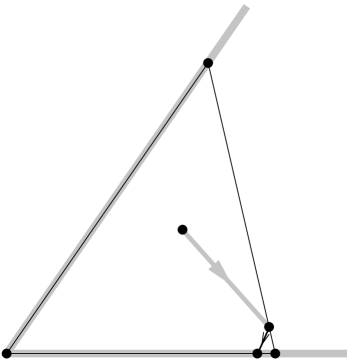
Figure 5: Corner divergences in the naive wedge–based derivation: perturbation about the wedge solution based on vertex 0.

Carrying through the derivation regardless, one obtains 6 coupled equations for 3 unknown functions. This is an overspecified system, as is most readily seen by discretising the result to obtain a problem of linear algebra. It is possible to remove the short distance problems by taking advantage of this overspecification.

3.3 “Regularising” the singular nature

We begin by adding an extra vertex on each side of the triangle so that Figure 2 becomes Figure 6. In this manner we regard the triangle as a degenerate 6–sided polygon. The manner in which the sides are subdivided is arbitrary but, as we will discuss later, there will be an optimal subdivision.

\psfrag{0}{$0$}\psfrag{1}{$1$}\psfrag{2}{$2$}\psfrag{3}{$3$}\psfrag{4}{$4$}\psfrag{5}{$5$}\psfrag{P0}{\Large$\boldsymbol{P}_{0}$}\psfrag{P1}{\Large$\boldsymbol{P}_{1}$}\psfrag{P2}{\Large$\boldsymbol{P}_{2}$}\psfrag{P3}{\Large$\boldsymbol{P}_{3}$}\psfrag{P4}{\Large$\boldsymbol{P}_{4}$}\psfrag{P5}{\Large$\boldsymbol{P}_{5}$}\psfrag{l0}{$l_{0}$}\psfrag{l1}{$l_{1}$}\psfrag{l2}{$l_{2}$}\psfrag{l3}{$l_{3}$}\psfrag{l4}{$l_{4}$}\psfrag{l5}{$l_{5}$}\psfrag{phi0}{$\phi_{0}$}\psfrag{phi2}{$\phi_{2}$}\psfrag{phi4}{$\phi_{4}$}\includegraphics[height=188.62654pt]{WedgeNotation.eps}

Figure 6: Notation: Wedge–based integral equation

The boundary is now parameterised in 6 segments

$$\boldsymbol{r}_{\mu}(s)=\boldsymbol{P}_{\mu}+\frac{\boldsymbol{P}_{\mu+1}-\boldsymbol{P}_{\mu}}{|\boldsymbol{P}_{\mu+1}-\boldsymbol{P}_{\mu}|}\,s\quad 0<s<l_{\mu}$$ (3.2)

where $\mu=0,1,2,3,4,5$ and $\boldsymbol{P}_{6}\equiv\boldsymbol{P}_{0}$ in a natural cyclic manner. We denote the outward normals by $\boldsymbol{n}_{0}=\boldsymbol{n}_{1}$, $\boldsymbol{n}_{2}=\boldsymbol{n}_{3}$ and $\boldsymbol{n}_{4}=\boldsymbol{n}_{4}$.

The three wedge solutions about which one can perturb are now associated with verticies $0$, $2$ and $4$. Let us consider the perturbation about $W_{0}(\boldsymbol{x},\boldsymbol{x}_{f})$.

Define

$$X_{\mu}(t) =\nabla T(\boldsymbol{r}_{\mu}(t),\boldsymbol{x}_{i})\,.\,\boldsymbol{n}_{\mu} 0<t<l_{\mu}$$ (3.3a)

$$X^{0}_{\mu}(t) =2\nabla W_{0}(\boldsymbol{r}_{\mu}(t),\boldsymbol{x}_{i})\,.\,\boldsymbol{n}_{\mu} 0<t<l_{\mu}$$ (3.3b)

where $\mu=0,1,2,3,4,5$ and

$$K_{\mu\nu}(t,s)=-2\nabla W_{0}(\boldsymbol{r}_{\nu}(s),\boldsymbol{r}_{\mu}(t))\,.\,\boldsymbol{n}_{\mu}\quad\quad\quad 0<t<l_{\mu}\,,\quad 0<s<l_{\nu}$$ (3.4)

where $\mu=0,1,4,5$ and $\nu=2,3$. (2.5) then gives the pre–integral equation.

$$T(\boldsymbol{x}_{f},\boldsymbol{x}_{i})=W_{0}(\boldsymbol{x}_{i},\boldsymbol{x}_{f})+\int_{0}^{l_{2}}W_{0}(\boldsymbol{r}_{2}(s),\boldsymbol{x}_{f})\,X_{2}(s)\,ds+\int_{0}^{l_{3}}W_{0}(\boldsymbol{r}_{3}(s),\boldsymbol{x}_{f})\,X_{3}(s)\,ds$$ (3.5)

There are now 4 possible boundary limits. Defining a diagramatic notation analogous to that given in Figure 3 we illustrate 2 typical boundary limits in Figure 7. Taking the limit to sides $0$ and $5$ it is clear that there is a lower bound on the propagation distance. This is not the case taking the limit to sides $1$ and $4$. We take advantage of the overspecification, only using the non–singular limits.

\psfrag{0}{$0$}\psfrag{1}{$1$}\psfrag{2}{$2$}\psfrag{3}{$3$}\psfrag{4}{$4$}\psfrag{5}{$5$}\psfrag{P0}{\Large$\boldsymbol{P}_{0}$}\psfrag{P1}{\Large$\boldsymbol{P}_{1}$}\psfrag{P2}{\Large$\boldsymbol{P}_{2}$}\psfrag{P3}{\Large$\boldsymbol{P}_{3}$}\psfrag{P4}{\Large$\boldsymbol{P}_{4}$}\psfrag{P5}{\Large$\boldsymbol{P}_{5}$}\includegraphics[height=188.62654pt]{WedgeBLNonSing.eps}

(a) Non–Singular boundary limit

\psfrag{0}{$0$}\psfrag{1}{$1$}\psfrag{2}{$2$}\psfrag{3}{$3$}\psfrag{4}{$4$}\psfrag{5}{$5$}\psfrag{P0}{\Large$\boldsymbol{P}_{0}$}\psfrag{P1}{\Large$\boldsymbol{P}_{1}$}\psfrag{P2}{\Large$\boldsymbol{P}_{2}$}\psfrag{P3}{\Large$\boldsymbol{P}_{3}$}\psfrag{P4}{\Large$\boldsymbol{P}_{4}$}\psfrag{P5}{\Large$\boldsymbol{P}_{5}$}\includegraphics[height=188.62654pt]{WedgeBLSing.eps}

(b) Singular boundary limit

Figure 7: Boundary limit of wedge pre–integral equation (3.5) to two typical segments. The integration over sides 2 and 3 is schematically given to show the absence (presence) of short distance propagation in the boundary limit to 0 (1).

Perturbing about the wedge solutions associated with vertices $2$ and $4$ in an analogous manner gives a set of six coupled integral equations

$$X_{\mu}(t)=X_{\mu}^{0}(t)+\sum_{\nu=0}^{5}\int_{0}^{l_{\nu}}K_{\mu\nu}(t,s)X_{\mu}(s)\,ds$$ (3.6)

Of the 36 possible $K_{\mu\nu}$ only the following 12 are non zero

$$K_{\mu,\mu+2},K_{\mu,\mu+3} \quad\quad\mu\text{ even}$$ (3.7a)

$$K_{\mu,\mu+3},K_{\mu,\mu+4} \quad\quad\mu\mbox{ odd }$$ (3.7b)

where addition is modulo $6$. These quantum pruning rules are easier to remember using the diagrammatic form of the integral equations. The kernel $K_{\mu\nu}$ is constructed using the wedge solution whose vertex is closest to the side corresponding to the first index.

Perturbing about the wedge thus gives us a closed set of non–singular integral equations for the unknown normal derivative. The Fredholm theory guarantees that these equations define the unknown normal derivative uniquely. Substituting this solution into the pre–integral equation then gives the solution of the boundary value problem (1.1).

In a sense, the need to start from the wedge solution is quite appealing because it gives a “bootstrap” character to the solution of boundary value problems: the triangle is solved in terms of the wedge problem; the wedge in terms of the free Green’s function. One is led to think how the triangle solution might be used in constructing even more complicated solutions (perhaps the tetrahedron).

3.4 Validation

Although the derivation has been straightforward and the result is more or less clear, it is nevertheless important to validate our approach. The first step towards this is to carry out a standard numerical discretisation of the integral equations, calculating the Fredholm determinant and thus the spectrum. It is important to reproduce exactly known spectra and compare the results for general triangles with the singular approach. We shall do this in section 5.

In our numerical work we would like to be assured that any discrepencies, any problems, are entirely due to the formulation of the integral equations. It is then important to be able to calculate the kernel of the wedge–based approach with well–controlled approximations. This requires a detailed understanding of the wedge kernel. It is to this that we now turn our attention.

4 Wedge Kernel

In appendix A we outline a derivation of the wedge Green’s function and obtain the following form of the wedge kernel (A.15)

$$\begin{split}K(r_{f},0;r_{i},\theta_{i};\phi)&\equiv-\nabla G_{W}(r_{f},0;r_{i},\theta_{i})\cdot\left(-\hat{\theta}\right)\\ &=\frac{1}{\phi r_{f}}\int_{C}P(\theta_{i},\phi;\omega)\frac{i}{4}H_{1}^{(1)}(\mu\lambda(\omega))\mu\lambda^{\prime}(\omega)d\,\omega\end{split}$$ (4.1)

where

$$P(\theta_{i},\phi;\omega) =\frac{1}{1-e^{-i\pi(\theta_{i}+\omega)/\phi}}$$ (4.2a)

$$\cosh\alpha =\frac{1}{2}\left(\frac{r_{f}}{r_{i}}+\frac{r_{i}}{r_{f}}\right)$$ (4.2b)

$$\lambda(\omega) =\sqrt{\cosh\alpha-\cos\omega}$$ (4.2c)

$$\mu =\sqrt{2zr_{i}r_{f}}$$ (4.2d)

where the natural polar co–ordinate system has been used. $H_{1}^{(1)}$ is the first order Hankel function of the 1st kind. The square root in (4.2c) is the principal square root with a branch cut on the negative real axis. The contour $C$ together with the analytic structure of the integrand is given in Figure 8.

Using (4.1) we have e.g., $K_{01}(t,s)=K(t,r_{i}(s),\theta_{i}(s);\phi_{0})$ where $r_{i}$ and $\theta_{i}$ are obtained using elementary trigonometry. We shall use the term “wedge kernel” to refer to both (4.1) and $K_{\mu\nu}(t,s)$ as there is little danger of confusion.

\psfrag{E1}[t]{\footnotesize$-2\pi+i\alpha$}\psfrag{E2}[b][t]{\footnotesize$-2\pi-i\alpha$}\psfrag{E3}[t]{\footnotesize$i\alpha$}\psfrag{E4}[b][t]{\footnotesize$-i\alpha$}\psfrag{E5}[t]{\footnotesize$2\pi+i\alpha$}\psfrag{E6}[b][t]{\footnotesize$2\pi-i\alpha$}\includegraphics[height=188.62654pt]{wplane.eps}

Figure 8: Wedge kernel: Analytic structure of integrand and integration contours. The integrand decays at infinity in the lightly shaded regions. Heavy shading denotes branch cuts in $\lambda(\omega)$ and crosses represent the poles of $P(\theta,\phi,\omega)$. The dotted contour is the Carslaw contour $C$. For the semiclassical evaluation it is deformed to the solid contour which goes along the paths of steepest descent though $\pm\pi$.

4.1 How to calculate the contour integral

As with all special functions, the calculation of (4.1) has to proceed through controlled approximations. In general, a given approximation technique is only valid in a particular region of parameter space so that one must consider a range of techniques in order to be able to calculate the function globally. For (4.1) we basically have two regimes: the semiclassical regime, $|\sqrt{z}(\mathbf{x}_{f}-\mathbf{x}_{i})|\gg 1$, in which the method of steepest descents is suitable; and the quantum regime, $|\sqrt{z}(\mathbf{x}_{f}-\mathbf{x}_{i})|\ll 1$, where the standard eigenfunction series is suitable. By developing each technique sufficiently one can extend each of them, with sufficient computational effort, so that the two regimes overlap. We are then able to calculate (4.1) for all parameters.

Naturally, we are initially interested in an effective semiclassical approximation. Previous analyses [46, 47] were concerned with the scattering problem. The analysis for the Greens function is similar. However, because we require a controlled approximation it is neccessary to undertake a somewhat deeper treatment. Let us begin by outlining the standard semiclassical analysis.

4.2 Asymptotic analysis and geometrical optics interpretation

The semiclassical limit corresponds to $\mu\to\infty$. In this limit the integrand is dominated by $e^{i\mu\lambda(\omega)}$ so that the method of steepest descents is appropriate. One readily locates saddle points at $\pm\pi$ together with the local path of steepest descent. Deforming the Carslaw contour $C$ to the steepest descent contours one collects contributions from the real poles in the region $-\pi<\operatorname{Re}(\omega)<\pi$ (Figure 8). The pole contributions are of geometrical optics form, i.e. a free Green’s function in which the distance, $|\mathbf{x}_{f}-\mathbf{x}_{i}|$, is generalised to include paths from $\mathbf{x}_{i}$ to $\mathbf{x}_{f}$ via classically possible collisions with the walls. All possible classical paths are represented with an appropriate phase for the corresponding free Green’s function. The remaining contour integrals, in the steepest descent approximation, can be interpreted in terms of a classical path from $\mathbf{x}_{i}$ to $\mathbf{x}_{f}$ via the vertex. The importance of such paths, which are not classical but nevertheless minimise the action, was recognised by Keller [1] in his geometrical theory of diffraction.

The steepest descent integrations are not uniformly of Gaussian form. The poles, located at $2n\phi-\theta_{i}$, $(n\in\mathbb{Z})$, pass through the the steepest descent contour at certain values of $\theta_{i}$ so that the number of geometrical optics terms varies. This simply corresponds to the motion of the “shadow” of the source point. This apparently discontinuous behaviour is of course an artifact of the method of steepest descent. It is well known that the geometric terms “switch on” with an error function modulation. This is the Stokes’ phenomenon and a uniform approach to it has been studied in recent years [50]. A uniform approach to a special case of the scattering problem was given by Pauli [46].

It would be natural at this point to derive asymptotic series. This only requires a local knowledge of the integrand (in particular the steepest descent contour) at the saddle points and at infinity. In order to determine the nature of the error and, if possible, bound it, this understanding needs to be global. Because such an analysis is rarely presented we shall give it in some detail.

While we could in principle carry out an error analysis for the asymptotic series, this is not really neccessary for our purposes. Asymptotic series are useful to understand the asymptotic form of the results. We already understand this through the standard interpretation in terms of (generalised) classical paths. All we require is well–controlled approximations in order to validate the non–singular integral equation. This is conveniently and practically obtained via Gauss-Hermite quadrature along the steepest descent contour. Numerical quadrature along any other contour gives poor convergence due to oscillations in the integrand. (This is of course the rationale behind the steepest descent method.) We only know of one other study which uses the method of steepest descents as the basis of a numerical quadrature [48, p.265].

4.3 Global understanding of integrand: $\omega\leftrightarrow t$ transformation

The steepest descent contour $\omega(t)$ is defined implicitly by

$$\lambda(\omega)=\lambda_{0}+\frac{it^{2}}{\mu},\quad\quad-\infty<t<\infty$$ (4.3)

where $\lambda_{0}=\sqrt{\cosh\alpha+1}$. Rather than regard the variable $t$ as a parameterisation of the steepest descent contour, consider (4.3) to define a transformation to a complex $t$–plane. In the $t$–plane the contour is simply along the real axis. The integrand is of a semiclassical form only if it is a well peaked Gaussian in the $t$ variable.

Let us first write the conformal transformation (4.3) in the following dimensionless manner

$$\frac{it^{2}}{\eta}=\sqrt{1-\frac{1+\cos\omega}{\sigma}}-1$$ (4.4)

where

$$\eta =\mu\lambda_{0}=\sqrt{z}(r_{i}+r_{f})$$ (4.5a)

$$\sigma =\lambda_{0}^{2}=1+\cosh\alpha$$ (4.5b)

$\eta$ is essentially a dimensionless wave vector. The semiclassical limit is conventionally regarded as $\eta\gg 1$, corresponding to a de Broglie wavelength which is small compared to typical distances in the problem. The parameter $\sigma$ is a purely geometrical, scale invariant parameter. $\sigma\gg 1$ indicates that that one of the distances $r_{i},r_{f}$ is much larger than the other, i.e. that one of them is “close” to the corner. As we shall see the semiclassical limit requires not only the conventional $\eta\gg 1$ but also requires $\sigma\ll 1$.

$\omega\leftrightarrow t$ can be constructed via the sequence of transformations $\omega\leftrightarrow u$, $u\leftrightarrow v$, and $v\leftrightarrow t$ where

$$u =\frac{1+\cos\omega}{\sigma}$$ (4.6a)

$$\frac{iv}{\eta} =\sqrt{1-u}-1$$ (4.6b)

$$t^{2} =v$$ (4.6c)

The choice of variable $u$ is suggested by the fact that $u=0$ at the saddle point and turns out to be convenient. The other choices are more or less natural.

$\omega\leftrightarrow t$ is summarised in Figure 9. The sequence of transformations leading to it is described in Figures 9(a), 10, 11 and 12. The transformation is visualised by following features in the $\omega$ plane through the transformation sequence. It is also convenient to follow the quadrants of the $u$ plane. Arrows are used to denote how various branches should be glued together. For example in Figure 9(a) we have a arrow labelled with a solid circle which crosses the line $\operatorname{Im}(\omega)=\pi,\operatorname{Re}(\omega)>0$. In Figure 10 we show the corresponding motion between branches of $u(\omega)$.

Let us first consider $\omega\leftrightarrow u$. The images of the $u$ quadrants in the $\omega$ plane are determined in the following manner. The images of the real and imaginary $u$ axes are readily determined. They partition the $\omega$–plane. One can identify which region corresponds to which quadrant of the $u$–plane by using the asymptotic result $u=1+\cos\omega\sim 1+\tfrac{1}{2}e^{\mp i\operatorname{Re}(\omega)}$ as $\operatorname{Im}(\omega)\to\pm\infty$ and continuity. The transformation is clearly multivalued. Single valued transformations (branches) $\omega(u)$ can be obtained by restricting the domain of $\omega$. This can be done in an infinite number of ways so that we have the luxury of choosing the most convenient. For example we can partition the $\omega$ plane into the regions $n\pi<\operatorname{Re}(\omega)<(n+1)\pi$, $n\in\mathbb{Z}$. Each region maps into the $u$–plane in a $1\leftrightarrow 1$ manner. Alternatively could choose the partition $2n\pi<\operatorname{Re}(\omega)<2(n+1)\pi$, $\operatorname{Im}(\omega)>0$ and $2n\pi<\operatorname{Re}(\omega)<2(n+1)\pi$, $\operatorname{Im}(\omega)<0$, $n\in\mathbb{Z}$. Any set of curves can be used in to partition the $\omega$ plane provided the regions obtained each cover the entire $u$ plane once. The convenient partition for our purposes is the first choice. In Figures 9(a) and 10 we show the transformation for the $n=0$ and $n=1$ branches. It will become apparent in due course that we need to follow two branches at a time. For the moment the reader should note that the steepest descent contour through $\pi$ occupies both branches.

\psfrag{E1}[lt][lt]{\footnotesize$i\alpha$}\psfrag{E2}[r][r]{\footnotesize$-i\alpha$}\psfrag{E3}[lt][lt]{\footnotesize$2\pi+i\alpha$}\psfrag{E4}[lt][lt]{\footnotesize$2\pi-i\alpha$}\psfrag{2Pi}[b][t]{\footnotesize$2\pi$}\psfrag{Pi}[b][t]{\footnotesize$\pi$}\psfrag{0}[b][t]{\footnotesize$0$}\psfrag{U1}{$\framebox{1}$}\psfrag{U2}{$\framebox{2}$}\psfrag{U3}{$\framebox{3}$}\psfrag{U4}{$\framebox{4}$}\psfrag{L1}{$\framebox{1}$}\psfrag{L2}{$\framebox{2}$}\psfrag{L3}{$\framebox{3}$}\psfrag{L4}{$\framebox{4}$}\includegraphics[height=188.62654pt]{w.eps}

(a) $\omega$–plane: Some features in $\omega\leftrightarrow u$ are also shown (see Figure 10). The $n=0$ ($n=1$) branch of this transformation corresponds to $0<\operatorname{Re}(\omega)<\pi$ ($\pi<\operatorname{Re}(\omega)<2\pi$). The bold dotted lines are images of the imaginary $u$ axis. The bold solid lines are images of the real $u$ axis. These lines partition the $\omega$–plane into regions. The correspondance between these regions and the quadrants of the $u$–plane is given by boxed numbers.

\psfrag{A}{A}\psfrag{B}{B}\psfrag{C}{C}\psfrag{D}{D}\psfrag{E}{E}\psfrag{F}{F}\psfrag{G}{G}\psfrag{E1}{-$\sqrt{i\eta}$}\psfrag{E2}{-$\sqrt{v_{c}}$}\psfrag{E3}{$\sqrt{v_{c}}$}\psfrag{E4}{$\sqrt{i\eta}$}\includegraphics[height=188.62654pt]{t.eps}

(b) $t$– plane. $v_{c}=i\sqrt{z}(r_{i}+r_{f}-|r_{f}-r_{i}|)$

Figure 9: $\omega\leftrightarrow t$ transformation: $n=0$ branch. Corresponding features in the two planes are labelled identically. Labelled arrows are used here and in other figures to indicate how branches are connected.

\psfrag{Q1}{\footnotesize$\framebox{1}$}\psfrag{Q2}{\footnotesize$\framebox{2}$}\psfrag{Q3}{\footnotesize$\framebox{3}$}\psfrag{Q4}{\footnotesize$\framebox{4}$}\psfrag{1}{\footnotesize$1$}\psfrag{A}{\footnotesize A}\psfrag{B}{\footnotesize B}\psfrag{C}{\footnotesize C}\psfrag{Uc}{\footnotesize$u_{c}$}\includegraphics[scale={0.5}]{u0.eps}

(a) $n=0$ branch

\psfrag{Q1}{\footnotesize$\framebox{1}$}\psfrag{Q2}{\footnotesize$\framebox{2}$}\psfrag{Q3}{\footnotesize$\framebox{3}$}\psfrag{Q4}{\footnotesize$\framebox{4}$}\psfrag{1}{\footnotesize$1$}\psfrag{D}{\footnotesize D}\psfrag{E}{\footnotesize E}\psfrag{F}{\footnotesize F}\psfrag{G}{\footnotesize G}\psfrag{Uc}{\footnotesize$u_{c}$}\includegraphics[scale={0.5}]{u1.eps}

(b) $n=1$ branch

Figure 10: $\omega\leftrightarrow u\leftrightarrow v\leftrightarrow t$ transformation: $u$ plane. $u_{c}=\frac{2}{\sigma}$

\psfrag{A}{\footnotesize A}\psfrag{B}{\footnotesize B}\psfrag{C}{\footnotesize C}\psfrag{iE}{\footnotesize$i\eta$}\psfrag{Vc}{\footnotesize$v_{c}$}\includegraphics[scale={0.45}]{v0.eps}

(a) $n=0$ branch

\psfrag{D}{\footnotesize D}\psfrag{E}{\footnotesize E}\psfrag{F}{\footnotesize F}\psfrag{G}{\footnotesize G}\psfrag{iE}{\footnotesize$i\eta$}\psfrag{Vc}{\footnotesize$v_{c}$}\includegraphics[scale={0.45}]{v1.eps}

(b) $n=1$ branch

Figure 11: $\omega\leftrightarrow u\leftrightarrow v\leftrightarrow t$ transformation: $v$ plane. $v_{c}=i\sqrt{z}(r_{i}+r_{f}-|r_{f}-r_{i}|)$. Analytic continuation into the darkly shaded regions corresponds to analytic continution through the cuts at $2n\pi\pm i\alpha,n\in\mathbb{Z}$ in the $\omega$–plane.

\psfrag{A}{\footnotesize A}\psfrag{B}{\footnotesize B}\psfrag{C}{\footnotesize C}\psfrag{iE}{\footnotesize$\sqrt{i\eta}$}\psfrag{Vc}{\footnotesize$\sqrt{v_{c}}$}\includegraphics[scale={0.45}]{t0.eps}

(a) $n=0$ branch

\psfrag{D}{\footnotesize D}\psfrag{E}{\footnotesize E}\psfrag{F}{\footnotesize F}\psfrag{G}{\footnotesize G}\psfrag{iE}{\footnotesize$-\sqrt{i\eta}$}\psfrag{Vc}{\footnotesize$-\sqrt{v_{c}}$}\includegraphics[scale={0.45}]{t1.eps}

(b) $n=1$ branch

Figure 12: $\omega\leftrightarrow u\leftrightarrow v\leftrightarrow t$ transformation: $t$ plane

$u\leftrightarrow v$ is readily constucted using a sequence of elementary transformations . The $v$-plane is given in Figure 11. An important feature to follow is the branch cut at $u=\frac{2}{\sigma}$. In the $v$–plane this becomes a vertical branch cut with the branch point at

$$v_{c}=\left\{\begin{array}[]{ll}2i\sqrt{z}r_{i}&\mbox{for $r_{f}>r_{i}$}\\ 2i\sqrt{z}r_{f}&\mbox{for $r_{i}>r_{f}$}\end{array}\right.$$ (4.7)

All that remains is $v\leftrightarrow t$. Although this is just a square root, some thought is necessary. Up until now we have used the symbol $\sqrt{\phantom{z}}$ with minimal explanation. In general this symbol denotes the standard square root, which has a branch cut along the negative real axis. Let us define another square root whose branch cut is along the negative imaginary axis. As this can be a point of confusion let us be very precise

$$\text{Let }z=|z|e^{i\theta},\text{ with }-\frac{\pi}{2}<\theta<\frac{3\pi}{2}.\text{ Then}\left.\sqrt{z}\right|_{-i\infty}=|z|^{1/2}e^{i\theta/2},$$ (4.8)

We map the $n=0$ copy of the $v$–plane to the $t$–plane using $v=\left.\sqrt{z}\right|_{-i\infty}$ and the $n=1$ copy of the $v$–plane to the $t$–plane using $v=-\left.\sqrt{z}\right|_{-i\infty}$. We show the results in Figure 12 where it is clear that we can paste the two regions together. The arrows indicate that this can be done in an analytic manner to give a $1\leftrightarrow 1$ map of $0<\operatorname{Re}(\omega)<2\pi\leftrightarrow$ (most of the) $t$–plane. We denote this as $\omega_{0}(t)$ and call it the principal branch.

Let us then summarise algebraically. We transform from $\omega$ to $t$ using

$$u=\frac{1+\cos\omega}{\sigma}$$ (4.9a)

$$v=-i\eta(-1+\sqrt{1-u})$$ (4.9b)

$$t=\begin{cases}\phantom{-}\left.\sqrt{v}\right|_{-i\infty}&0<\operatorname{Re}(\omega)<\pi\\ -\left.\sqrt{v}\right|_{-i\infty}&\pi<\operatorname{Re}(\omega)<2\pi\end{cases}$$ (4.9c)

and from $t$ to $\omega$ using

$$v=t^{2}$$ (4.10a)

$$u=1-\left(1+\frac{iv}{\eta}\right)^{2}$$ (4.10b)

$$\omega=\begin{cases}\arccos(u\sigma-1)&-\tfrac{\pi}{4}<\arg(t)<\tfrac{3\pi}{4}\\ 2\pi-\arccos(u\sigma-1)&-\tfrac{5\pi}{4}<\arg(t)<-\tfrac{\pi}{4}\end{cases}$$ (4.10c)

where we have used the principal branch of $\omega=\arccos(z)$. This maps the $z$–plane into the region $0<\operatorname{Re}(\omega)<\pi$. The other branches of the partition are obtained in a similar manner. In fact one can readily see that $w_{n}(t)=2n\pi+w_{0}(t)$, $n\in\mathbb{Z}$. The steepest descent contour occupying $0<\operatorname{Re}(\omega)<2\pi$ (with orientation given in Figure 8) is mapped to the path in the $t$–plane along the real axis from $\infty$ to $-\infty$.

We can now see that it is not just the poles which spoil the Gaussian form of the integrand. When $\min(|zr_{f}|,|zr|)\ll 1$ (i.e. $\sigma\gg 1$) the cut at $\sqrt{v_{c}}$ collapses into the origin spoiling the Gaussian form of the integrand. This is the origin of the more subtle, non–semiclassical behaviour previously mentioned. At first sight it might appear that our formalism is always semiclassical, with its natural cutoff guaranteeing that $r_{f}+r_{i}$ has a minimum value of macroscopic magnitude. However because $r_{f}$ and $r_{i}$ are not so bounded from below there remain benign but nevertheless fully quantum contributions in the corners.

4.4 Uniform calculation of integral

Deforming $C$ to the steepest descent contour and changing integration variables to $t$, we readily obtain

$$\textrm{Pole Terms}-K^{(0)}(r_{f},r_{i},\theta_{i})+K^{(-1)}(r_{f},r_{i},\theta_{i})$$ (4.11)

where

$$K^{(n)}(r_{f},r_{i},\theta_{i})=\int_{-\infty}^{\infty}P^{(n)}(t)f(t)e^{-t^{2}}dt$$ (4.12)

and

$$P^{(n)}(t) =P(\theta_{i},\phi,\omega_{n}(t))$$ (4.13a)

$$f(t) =-\frac{1}{2\phi r_{f}}tH_{1}^{(1)}(\eta+it^{2})e^{t^{2}}$$ (4.13b)

The integrations (4.12) are now in standard Gaussian form.

For our purposes the most convenient way to proceed is to evaluate the integrals numerically using Gauss–Hermite quadrature. The quadrature converges well if $f(t)P(t)$ is a smooth, slowly varying function. Because our construction guarantees that $\eta$ is reasonably large, this is true for $f(t)$. $P(t)$ however has poles and this condition doesn’t apply when the poles are close to the real axis. This corresponds to $\boldsymbol{x}_{f}$ being in the penumbral region [49] so that the Gaussian approximation breaks down (see also [35, Figure 11.9]). We found that the presence of “close” poles spoiled the quadrature to an unacceptable degree for a significant number of matrix elements. It thus seems neccessary to handle such cases separately using some an alternative numerical method. Fortunately, as we have mentioned, this is essentially a Stokes’ phenomenon so that we are able to isolate the penumbral behaviour using well known uniform approaches [50, 51, 52, 46].

The basic idea is to analytically subtract the poles out of $P^{(i)}(t)$. This can be done a number of ways, the simplest being a recursive construction. Suppose we wish to subtract out poles at $\{\omega_{0},\omega_{1},\omega_{2},\ldots,\omega_{N}\}$. Let $t_{n}=t(\omega_{n})$ and form (temporarily dropping the superscript)

$$Q_{0}(t)=P(t)(t-t_{0})$$ (4.14)

Defining

$$P_{0} =Q_{0}(t_{0})$$ (4.15a)

$$R_{0}(t) =\frac{Q_{0}(t)-P_{0}}{t-t_{0}}$$ (4.15b)

we obtain

$$P(t)=\frac{P_{0}}{t-t_{0}}+R_{0}(t)$$ (4.16)

The pole at $t_{0}$ is thus isolated as a simple pole in the first term. We can recursively subtract off other poles. Suppose that $N-1$ poles have already been subtracted off. Form

$$Q_{N}(t)=R_{N-1}(t)(t-t_{N})$$ (4.17)

and define

$$P_{N} =Q_{N}(t_{N})$$ (4.18a)

$$R_{N}(t) =\frac{Q_{N}(t)-P_{N}}{t-t_{N}}$$ (4.18b)

we readily obtain

$$P(t)=\sum_{n=0}^{N}\frac{P_{n}}{t-t_{n}}+R_{N}(t)$$ (4.19)

Although it is not immediately apparent from the construction, $P_{n}$ is the residue of $P(t)$ at $t_{n}$. This is obvious from other arguments in complex analysis. Evaluating the residue we get

$$P_{n}=-\frac{\mu\phi}{4\pi}\frac{\sin\omega_{n}}{\lambda(\omega_{n})t_{n}}$$ (4.20)

It is natural to order the poles according to their proximity to the real axis and to subtract them out in this order. Plotting $R_{n}(t)$ after each subtraction we noted the smoothing effect. As the proceedure is straightforward all the poles in the $t$–plane were subtracted out .

We now proceed with the uniform analysis of the wedge kernel. Deform the Carslaw contour toward the steepest descent contour but this time don’t cross the poles. This gives two contours $T_{0}$ and $T_{-1}$ which are totally contained in the $n=0$ and $n=-1$ branches of the $\omega$–plane. Rewrite (4.12) as

$$I^{(-1)}(r_{f},r_{i},\theta_{i})-I^{(0)}(r_{f},r_{i},\theta_{i})$$ (4.21)

where

$$I^{(n)}(r_{f},r_{i},\theta_{i})=\int_{T_{i}}P^{(n)}(t)f(t)e^{-t^{2}}dt$$ (4.22)

The image of $T_{0}$ $(T_{-1})$ in the $t$–plane is a contour which goes from $-\infty$ to $\infty$ passing over (under) all the poles under (over) the cut at $(-)\sqrt{v_{c}}$.

Using (4.19) and performing one last one last pole subtraction we can write the integrand for $n=0$ as

$$P^{(0)}(t)f(t)=\sum_{0<\operatorname{Re}(\omega_{n})<2\pi}\frac{P^{(0)}_{n}f(t_{n})}{t-t_{n}}+\sum_{0<\operatorname{Re}(\omega_{n})<2\pi}P^{(0)}_{n}\frac{f(t)-f(t_{n})}{t-t_{n}}+R^{(0)}_{N}(t)$$ (4.23)

with a similar result for $n=-1$. The integration is analogously decomposed into three terms. The absence of poles in the last two terms allows us to deform the contour $T_{i}$ to the real axis. Using

$$\int_{T_{0}}\frac{e^{-t^{2}}dt}{t-z} =\phantom{-}i\pi w(z)\phantom{-}\quad z\text{ above }T_{-1}$$ (4.24a)

$$\int_{T_{-1}}\frac{e^{-t^{2}}dt}{t-z} =-i\pi w(-z)\quad z\text{ below }T_{0}$$ (4.24b)

(Ref. [40], Chapter 7) we finally obtain

$$\begin{split}K(r_{f},r_{i},&\theta_{i};\phi)=\\ &\sum_{0<\operatorname{Re}(\omega_{n})<2\pi}i\pi P^{(0)}_{n}f(t_{n})w(-t_{n})\quad+\sum_{-2\pi<\operatorname{Re}(\omega_{n})<0}i\pi P^{(-1)}_{n}f(t_{n})w(t_{n})\\ &-\sum_{0<\operatorname{Re}(\omega_{n})<2\pi}P^{(0)}_{n}\int_{-\infty}^{\infty}\frac{f(t)-f(t_{n})}{t-t_{n}}e^{-t^{2}}\,dt\\ &+\sum_{-2\pi<\operatorname{Re}(\omega_{n})<0}P^{(-1)}_{n}\int_{-\infty}^{\infty}\frac{f(t)-f(t_{n})}{t-t_{n}}e^{-t^{2}}\,dt\\ &+\int_{-\infty}^{\infty}\left(R^{(-1)}_{N^{(-1)}}(t)-R^{(0)}_{N^{(0)}}(t)\right)e^{-t^{2}}\,dt\end{split}$$ (4.25)

where $N^{(0)}$ ($N^{(-1)}$) is the number of poles in the $n=0$ ($n=-1$) $t$–plane.

(4.25) is quite an interesting form. In the first two sums the contributions from the poles satisfying $-\pi<\operatorname{Re}(\omega_{n})<\pi$ are the geometrical optics terms, modulated by an error function. In this regime the asymptotic expansion of the error function has an exponential term which combines with the other factors to give the standard geometrical optics term. The first two sums also contain other poles. In the region containing these poles the exponential term is absent from the asymptotic expansion of the error function due to Stokes’ phenomenon and the resulting terms in the sum are of higher order. We shall refer to the first two sums as the uniform geometric contribution to the wedge kernel.

The “pole near a contour” problem is now isolated in the (well documented) error function. The remaining terms contain relatively smooth integrands and can be evaluated in a straightforward manner using Gauss–Hermite quadrature. They can also be evaluated asymptotically by expanding the integrands around the origin.

A priori, one would now expect to have to consider the case $\min(|zr_{f}|,|zr|)\ll 1$. As is clear from Figure 9(b), the semiclassical approach is not suitable in this “quantum” regime in which one should use the standard eigenfunction series. In Section 5 it will turn out that the parameter $\min(|zr_{f}|,|zr|)$ never gets small enough to require the use of this series.

5 Validation: Numerical Results

5.1 Numerical discretisation

The solution of integral equations via quadrature is a standard numerical technique described in many textbooks and with a vast research literature. The basic idea is to first choose some quadrature rule to approximate the integration. From here one readily obtains an inhomogenous linear equation for the unknown function at the quadrature nodes. This equation can then be solved using standard methods of numerical linear algebra. One then increases the number of nodes to achieve sufficient convergence.

In this section our main purpose is to validate the wedge–based approach. To do this we content ourselves with the determination of the first dozen or so eigenvalues for some typical triangles. This can be done comfortably using a quadrature similar to that used by Berry and Wilkinson [27] and carrying out the calculation entirely within the Mathematica package [53]. Most cases could be done with an overnight run on a standard workstation.

We expect that one should be able to use more sophisticated approaches very profitably in the wedge–based case. We don’t expect this to be so for the singular case.

5.2 Quadrature

The geometric nature of the integration variable, being an arc length along the boundary, allows one to readily visualise the quadrature. In order to keep things simple, we consider cases where the boundary is a uniform 1–dimensional lattice. The length of each side is given as an integer multiple of some of a lattice spacing $\epsilon$ and we give these lengths in the form of a triple, $\{n_{0},n_{1},n_{2}\}$. For example, the Pythagorean triangle with sides $1,\frac{4}{3}$ and $\frac{5}{3}$ can be specified by the triple $\{3,4,5\}$ with a lattice spacing of $\epsilon=\frac{1}{3}$. This defines 12 quadrature nodes. We take $\{n_{0},n_{1},n_{2}\}$ and $\epsilon$ to define a base quadrature. We refine this quadrature to $d_{f}\{n_{0},n_{1},n_{2}\}$ and $\epsilon/d_{f}$ where the discretisation factor $d_{f}$ is taken through the values $2,3,4,\ldots$ in order to demonstrate convergence. For the wedge–based case we need to specify a subdivision point for each side. This is readily accomodated in an obvious manner with the notation $\{\{n_{0},n_{1}\},\{n_{2},n_{3}\},\{n_{4},n_{5}\}\}$.

The quadrature nodes are chosen to lie at the midpoint of each unit cell so that the simplest quadrature is the midpoint rule. Our initial instinct was to avoid using the corners as quadrature points.

5.3 Computational effort

In order for the quadrature to be a good approximation it is necessary that one chooses enough nodal points so that the oscillations in the kernel are well sampled. The kernel oscillates with a wave number of the order $\sqrt{z}L$ where $L$ denotes a typical length scale for the triangle. A successful quadrature then requires the total number of nodes $n_{t}$ to be much larger than $\sqrt{z}L$. Li and Robnik [39] use a parameter $b=2\pi n_{t}/(\sqrt{z}L)$ which gives the number of number of nodes within one de Broglie wavelength. An effective discretisation requires $n_{t}\gg\sqrt{z}L$ or $b\gg 1$.

A discretisation of order $n_{t}$ requires $O(n_{t}^{2})$ operations to evaluate the kernel and then $O(n_{t}^{3})$ operations to evaluate the determinant. In our work the Bessel function evaluations were the most expensive part of the calculation so that effort grew quadratically in $\sqrt{z}L$. As higher energies are considered the effort will eventually cross over to the cubic regime.

5.4 Results

The eigenvalues are determined from the zeros of the Fredholm determinant, $\det(1-K)$, which we approximate using the discrete form of the kernel defined by our quadrature.

We consider in detail two cases: the equilateral triangle and the Pythagorean 3-4-5 triangle. The former case is an integrable billiard and the eigenvalues are known exactly. The integrable cases are described in [27]. The latter case was chosen as a “typical” non–integrable billiard.

Let us first give an overview of the lower part of the spectrum for each case, presenting plots of the modulus of the Fredholm determinant for real energies. The cases considered are given in Table 1.

Abbreviation	Base Quadrature
free-equilateral	$\{4,4,4\},\epsilon=\frac{1}{4}$
free-345	$\{3,4,5\},\epsilon=\frac{1}{3}$
wedge-equilateral	$\{\{2,2\},\{2,2\},\{2,2\}\},\epsilon=\frac{1}{4}$
wedge-345	$\{\{2,1\},\{2,2\},\{3,2\}\},\epsilon=\frac{1}{3}$

Table 1: Base quadratures for cases considered together with a shorthand description.

\psfrag{df = 1}[Br][Br]{\footnotesize$d_{f}=1$}\psfrag{df = 2}[Br][Br]{\footnotesize$d_{f}=2$}\psfrag{df = 3}[Br][Br]{\footnotesize$d_{f}=3$}\psfrag{|Determinant|}{\footnotesize$|$Determinant$|$}\psfrag{Scaled Energy}[t][b]{\footnotesize Scaled Energy, $E_{s}$}\includegraphics[height=226.34993pt]{Free444.eps}

(a) Free–based Fredholm determinant

\psfrag{df = 1}[Br][Br]{\footnotesize$d_{f}=1$}\psfrag{df = 2}[Br][Br]{\footnotesize$d_{f}=2$}\psfrag{df = 3}[Br][Br]{\footnotesize$d_{f}=3$}\psfrag{|Determinant|}{\footnotesize$|$Determinant$|$}\psfrag{Scaled Energy}[t][b]{\footnotesize Scaled Energy, $E_{s}$}\includegraphics[height=226.34993pt]{Wedge444.eps}

(b) Wedge–based Fredholm determinant

Figure 13: Equilateral Triangle: solution of singular and non–singular integral equations by numerical discretisation. The energy has been scaled to facilitate easy comparision with the exact solution. The number of lattice spacings per deBroglie wavelength, $b=6d_{f}/\sqrt{E_{s}}$.

In all plots we have applied an appropriate energy scaling. For the integrable cases we have used a scaling which allows easy comparison with exact results. For the non–integrable cases we have used Weyl’s result for the density of states to scale the energy so as to give, on average, a unit eigenvalue density.

In Figure 13(a) we give the results for the free-equilateral case. The first thing one notices is that the determinant does not converge with increasing $b$ i.e. the continuum limit does not exist. Despite this, the variation of the determinant still clearly resolves the eigenvalues. The spectrum, given in appropriate units by $E=m^{2}+n^{2}-mn$, $1<n<m$, is reproduced. Cusp behaviour near the zeros indicates isolated eigenvalues and smooth behaviour indicates degeneracies.

The wedge-equilateral case is shown in Figure 13(b). Here one observes the convergence that Fredholm theory demands. One expects that the lack of convergence in the free–based case is due to the singular nature of the integral equations.

\psfrag{df = 1}[Br][Br]{\footnotesize$d_{f}=1$}\psfrag{df = 2}[Br][Br]{\footnotesize$d_{f}=2$}\psfrag{df = 3}[Br][Br]{\footnotesize$d_{f}=3$}\psfrag{|Determinant|}{\footnotesize$|$Determinant$|$}\psfrag{Scaled Energy}[t][b]{\footnotesize Scaled Energy, $E_{s}$}\includegraphics[height=226.34993pt]{Free345.eps}

(a) Free–based Fredholm determinant

\psfrag{df = 1}[Br][Br]{\footnotesize$d_{f}=1$}\psfrag{df = 2}[Br][Br]{\footnotesize$d_{f}=2$}\psfrag{df = 3}[Br][Br]{\footnotesize$d_{f}=3$}\psfrag{|Determinant|}{\footnotesize$|$Determinant$|$}\psfrag{Scaled Energy}[t][b]{\footnotesize Scaled Energy, $E_{s}$}\includegraphics[height=226.34993pt]{Wedge345.eps}

(b) Wedge–based Fredholm determinant: uniform geometric kernel

Figure 14: 3-4-5 Triangle: solution of singular and non–singular integral equations by numerical discretisation. The energy has been scaled to given a unit density of states. The number of lattice spacings per deBroglie wavelength, $b=4.3d_{f}/\sqrt{E_{s}}$.

In Figures 14(a) and  14(b) we show the corresponding results for the 3-4-5 triangle. Once again the determinant doesn’t converge in the free case. We have used the uniform–geometric component of the wedge kernel. As we shall see this gives accurate results.

\psfrag{Energy2}[Br][Br]{\footnotesize$E_{s}=\phantom{1}2.0$}\psfrag{Energy6}[Br][Br]{\footnotesize$E_{s}=\phantom{1}6.0$}\psfrag{Energy10}[Br][Br]{\footnotesize$E_{s}=10.0$}\psfrag{logdf}[t][b]{\footnotesize$\log d_{f}$}\psfrag{logDet}{\footnotesize$\log|\det(d_{f})|$}\includegraphics[height=188.62654pt]{Conv345.eps}

Figure 15: Convergence in free–based case: $\log-\log$ plot of the modulus of the Fredholm determinant as a function of discretisation factor $d_{f}$, $|\det(d_{f})|$, at fixed energy for the 3-4-5 triangle.

In order to examine convergence more closely in the free–based approach, we show in Figure 15 a $\log-\log$ plot of the absolute value of the determinant versus the discretisation factor at some particular values of the energy for the 3-4-5 triangle. It is clear that the determinant decreases with $d_{f}$ in a power law manner with a exponent $\approx-1.5$. The exponent appears to be relatively uniform in energy. One could thus arrest the lack of convergence with an ad–hoc “renormalisation” factor.

\psfrag{Energy2.5}[Br][Br]{\footnotesize$E_{s}=\phantom{1}2.5$}\psfrag{Energy7.5}[Br][Br]{\footnotesize$E_{s}=\phantom{1}7.5$}\psfrag{Energy12.5}[Br][Br]{\footnotesize$E_{s}=12.5$}\psfrag{logdf}[t][b]{\footnotesize$\log d_{f}$}\psfrag{logDiffDet}{\footnotesize$\log|\det(d_{f}+1)-\det(d_{f})|$}\includegraphics[height=188.62654pt]{Conv444.eps}

Figure 16: Convergence in wedge–based case: $\log-\log$ plot of the first difference of the Fredholm determinant as a function of discretisation factor $d_{f}$, $|\det(d_{f}+1)-\det(d_{f})|$, at fixed energy for the 3-4-5 triangle.

In Figure 16 we quantify the convergence of the wedge–based approach by showing a $\log-\log$ plot of the first difference of the discretised Fredholm determinant versus $d_{f}$ for the equilateral triangle. The power law exponent is approximatly -3, which is consistent with the use of the midpoint rule. The straightness of the plot indicates that standard methods to accelerate convergence should work well.

\psfrag{Free df2}[Br][Br]{\footnotesize F, $d_{f}=2$}\psfrag{Free df3}[Br][Br]{\footnotesize F, $d_{f}=3$}\psfrag{Free df4}[Br][Br]{\footnotesize F, $d_{f}=4$}\psfrag{WedgeGeom df2}[Br][Br]{\footnotesize WG, $d_{f}=2$}\psfrag{WedgeUnifGeom df2}[Br][Br]{\footnotesize WU, $d_{f}=2$}\psfrag{WedgeFull df2}[Br][Br]{\footnotesize W, $d_{f}=2$}\psfrag{|Determinant|}{\footnotesize$|$Determinant$|$}\psfrag{Energy}[t][b]{\footnotesize Scaled Energy, $E_{s}$}\includegraphics[height=188.62654pt]{345Detail3.eps}

Figure 17: Fredholm determinants in the vicinity of the 3rd eigenvalue of the 3-4-5 triangle: detailed comparision of singular and non–singular approaches. For the latter the effect of approximations in the wedge kernel is also shown. F = free–based; WG = wedge–based, geometric kernel; WU = wedge–based, uniform geometric kernel; W = wedge-based with full kernel.

In Figure 17 we give detailed results in the vicinity of the 3rd eigenvalue of 3-4-5 triangle. We compare the geometric, uniform–geometric and full kernel–based approximations for the wedge–based method together with 3 discretisations of the free–based result. We see that the approximate wedge kernels give acceptable accuracy. We also note that the wedge–based and free–based methods agree very well in the location of the zeros.

To obtain 6 figure accuracy uniformly across all matrix elements for the full kernel we used an 8-point quadrature for the Gaussian integrals in (4.25). This is sufficient given the discretisation error in the numerical solution of the integral equation. This quadrature is relatively expensive due to the need for extra Bessel function evaluations.

As we mentioned at the end of Section 4, the semiclassical form of the wedge kernel is all we need. Because of the midpoint quadrature there is a minimum value of $r_{f}$ and $r_{i}$. Our modest numerical goals meant that the discretisation remained fairly coarse so that $\min(|zr_{f}|,|zr|)$ was never small enough to see the quantum regime.

In all figures one observes an expected decrease in the quality of eigenvalue determination as the quality of the discretisation $b$ decreases. Where direct comparision is possible the wedge–based code seems to resolve the eigenvalues better for a given $b$.

In some of the figures the curves are not perfectly smooth. This is due to the limited resolution of the plot. Each plot displays the determinant sampled at about 100 equally spaced points. The samples are connected with lines by the plotting routine gnuplot. Where the determinant varies quickly, such as near an eigenvalue, a higher resolution is needed. It is best to offer a separate plot in such regimes, as we have done in Figure 17. Such plots are needed to see the actual degree to which eigenvalues are resolved. For example in Figure 14(b) the third eigenvalue does not appear to be resolved very well. This is misleading because the the only energies sampled in this vicinity are $E_{s}=5.267$ and $5.333$. Figure 17 shows the true story. Also the power law decrease of the free determinant with $d_{f}$ artificially smoothens plots. This might falsely lead one to think that the free–based code gives better resolution that the wedge–based code. A “renormalisation” of the free results would give a fairer comparision.

5.5 Numerical checks

In order to develop confidence in our results we applied several checks in order to diminish the possiblity that numerical or coding errors were present. The first and most obvious check is the reproduction the exact spectrum for the equilateral triangle in both versions of the code. For the 3-4-5 case, and for nonintegrable triangles in general, there are no exact results for the eigenvalues. In these cases we apply consistency checks. Our main consistency check was to compare the results of the wedge–based code with the free–based code. We found that for the common eigenvalues, the agreement was very good. This can be seen in the case of the 3th eigenvalue in Figure 17. As a further check we also considered the free–354 and free–534 triangles, obtaining results identical to the free–345 case. To eliminate the presence of integrable wedges, we also considered the 2-3-4 triangle.

The lack of determinant convergence for the free-based code was originally thought to be possibly a result of coding error. The free–based code was originally intended as a “warm–up” exercise. After it was written we proceeded onto the more involved wedge-based calculation and improved the general quality of our software considerably. It was then relatively easy to modify the wedge–based code to produce, independently, a new version of the free–based code, which reproduced the original results. We further tested the free–based code by considering the other two integrable triangles: the isoceles right angled triangle (45,45,90) and the half–equilateral triangle (30,60,90). Our present code is written for triangles with rational sides. We thus considered the $\{12,12,17\}$ and $\{15,26,30\}$ triangles, with suitable values of $\epsilon$. These approximate the two cases to 1 part in 100. We found full agreement with the exact spectra.

6 Periodic Orbit Expansions

We now have a mathematically well behaved reformulation of the boundary value problem which has been well validated using numerical techniques.

An intuitive understanding of the high energy, semiclassical eigenvalues could now be obtained by deriving a periodic orbit expansion using the Fredholm series, much as Georgeot and Prange describe [22]. The calculation of the periodic orbit expansions is now a matter of using the semiclassical form of the wedge kernel to calculate $\operatorname{Tr}_{n}$ asymptotically. Similar analysis has been done in other contexts [29, 38]. In our case the analysis will differ due to the subdivision of the sides of the polygon and the uniform approach to the diffractive contribution.

It is more important to first examine the nature of the periodic orbit expansions using Fredholm theory. In particular we wish to compare the computational effort of the periodic orbit expansions with standard numerical discretisation.

6.1 Convergence of Fredholm series

Standard Fredholm theory [23, §6.5] shows that series for the Fredholm determinant,

$$\Delta(z)=\sum_{n=0}^{\infty}\;\delta_{n}(z),$$ (6.1)

is convergent by bounding $|\delta_{n}|$ using Hadamard’s inequality. From this bound one can readily estimate that $|\delta_{n}|$ increases until

$$n_{c}\approx\|K\|^{2}$$ (6.2)

after which it decreases. In practice one might then expect that at least $3n_{c}$ terms are needed in the Fredholm expansion.

In order to apply this result we need to understand the behaviour of the norm for all values of the energy. In particular it is clear that one has an effective semiclassical approximation if and only if the norm decreases with energy. The faster the rate of decrease the better.

It is relatively easy to estimate the norm in the semiclassical limit $\sqrt{z}|\boldsymbol{\Delta}_{\mu\nu}|\gg 1$. In this limit the wedge kernel is dominanted by geometric optics terms so that it has the form

$$K_{\mu\nu}(t,s)\sim-\frac{i}{\sqrt{2\pi}}\,z^{1/4}\sum_{\begin{subarray}{c}\text{\footnotesize classical}\\ \text{\footnotesize paths }\alpha\end{subarray}}\frac{e^{i(\sqrt{z}|\boldsymbol{\Delta}^{\alpha}_{\mu\nu}|-3\pi/4)}}{|\boldsymbol{\Delta}^{\alpha}_{\mu\nu}|^{1/2}}\frac{\boldsymbol{\Delta}^{\alpha}_{\mu\nu}\,.\,\boldsymbol{n}_{\mu}}{|\boldsymbol{\Delta}^{\alpha}_{\mu\nu}|}$$ (6.3)

The number of classical paths varies with $t$ and $s$ as the shadow of the source point moves. Diffractive contributions decay with a faster power law

The semiclassical norm then becomes

$$\|K\|^{2} \sim\sum_{\mu=0}^{5}\sum_{\nu=0}^{5}\int_{0}^{l_{\mu}}\,ds\int_{0}^{l_{\nu}}\,dt|K_{\mu\nu}(t,s)|^{2}$$ (6.4a)

$$\begin{split}=\frac{\sqrt{z}}{2\pi}\;\sum_{\mu=0}^{5}\sum_{\nu=0}^{5}\int_{0}^{l_{\mu}}\,ds\int_{0}^{l_{\nu}}\,dt\left(\sum_{\alpha}\left(\frac{\boldsymbol{\Delta}^{\alpha}_{\mu\nu}\,.\,\boldsymbol{n}_{\mu}}{|\boldsymbol{\Delta}^{\alpha}_{\mu\nu}|}\right)^{2}\frac{1}{|\boldsymbol{\Delta}^{\alpha}_{\mu\nu}|}\right.\\ \quad\quad\left.+\quad\sum_{\alpha\neq\beta}\frac{e^{i\sqrt{z}(|\boldsymbol{\Delta}^{\alpha}_{\mu\nu}|-|\boldsymbol{\Delta}^{\beta}_{\mu\nu}|)}}{|\boldsymbol{\Delta}^{\alpha}_{\mu\nu}|^{1/2}|\boldsymbol{\Delta}^{\beta}_{\mu\nu}|^{1/2}}\frac{\boldsymbol{\Delta}^{\alpha}_{\mu\nu}\,.\,\boldsymbol{n}_{\mu}}{|\boldsymbol{\Delta}^{\alpha}_{\mu\nu}|}\frac{\boldsymbol{\Delta}^{\beta}_{\mu\nu}\,.\,\boldsymbol{n}_{\mu}}{|\boldsymbol{\Delta}^{\beta}_{\mu\nu}|}\right)\end{split}$$ (6.4b)

$$=\sqrt{z}L+\text{ oscillatory terms }$$ (6.4c)

where $L$ is length of order the size of the triangle. The oscillatory terms come from a steepest descents evaluation of the integration over the second sum.

(6.3) is not uniformly valid for all $t$ and $s$. Although our technique avoids the unit source singularity there remains non–classical behaviour when one of $\sqrt{z}r_{i}$ or $\sqrt{z}r_{f}$ is very small. One expects that (6.3) will cross over into some other form in this boundary layer region. We have no reason to believe that incorporating the boundary layer contribution will dramatically alter the above estimation of the norm. To confirm this we generated $\log-\log$ plots of the norm versus energy and confirmed the above behaviour. However our discretisation was not fine enough, nor was our energy high enough, to see any boundary layer behaviour in the calculation of the kernel. It is thus conceivable that at higher energies some change in the norm behaviour may be observed.

We thus have

$$n_{c}\sim\sqrt{z}L$$ (6.5)

so that the number of terms needed grows with the square root of the energy. This accords with the literature on periodic orbit expansions but is not what one would expect of a semiclassical expansion.

6.2 The correspondance principle

In the old quantum theory Bohr presumed that any semiclassical approximation should improve in “the limit of large quantum numbers”. In our context one would expect that the semiclassical approximation should improve as energy increased. This is clearly not the case for periodic orbit expansions. The semiclassical Fredholm series is useful only if $\sqrt{z}L$ is large enough to use the semiclassical approximation for $\delta_{n}(z)$ but small enough so that not too many terms are needed.

We can offer an elementary analogy to impress apon the reader the true nature of periodic orbit expansions. Consider the asymptotic calculation of the zeros of the Bessel function, i.e. solve $J_{\nu}(z)=0$ for $z\to\infty$. The Bessel function can be defined in terms of series or integral representations. It is natural to handle this problem using the standard asymptotic result

$$J_{\nu}(z)\sim\sqrt{\frac{2}{\pi z}}\cos(z-\frac{1}{2}\nu\pi-\frac{1}{4}\pi)$$ (6.6)

Zeros obtained in this way are very accurate and improve in accuracy as $z\to\infty$. In actual fact the accuracy is acceptable right down to the ground state! ([40, 9.5.12]) A less natural way to proceed would be to use the series representation

$$J_{\nu}(z)=(\tfrac{1}{2}z)^{\nu}\,\sum_{k=0}^{\infty}\frac{(-\frac{1}{4}z^{2})^{k}}{k!\Gamma(\nu+k+1)}$$ (6.7)

because the number of terms need to obtain good convergence is of the order of $\frac{3}{2}z$. Finding eigenvalues from periodic orbit expansions is like using the power series expansions to find zeros of Bessel functions. It is clear then that

The problem of semiclassical quantisation of chaotic systems will not be solved until one has found the analog of (6.6).

6.3 Computational effort: comparison with discretisation

Let us now examine the computational effort needed to evaluate the semiclassical Fredholm series.

The number of terms need to obtain good convergence is of order the dimensionless wavenumber $\sqrt{z}L$. A semiclassical calculation of $\delta_{n}$ involves all periodic orbits with $n$ bounces for the triangular billiard. The number of such orbits is known to grow polynomially in $n$ [25]. The order of this polynomial is not known but there are some conjectures. For integrable triangles it is relatively easy to see that the growth is linear. Either way the computational effort required to calculate high energy eigenvalues grows polynomially in $\sqrt{z}L$. Discretisation of the boundary integral equation requires computational effort which grows like $(\sqrt{z}L)^{3}$ although in our case, as we discussed in Section 5, it was effectively quadratic. This becomes comparable to the semiclassical Fredholm series for integrable billiards. For generic billiards we would expect the effort to be qualitatively comparable

This is in contrast to the case of chaotic smooth billiards. Our estimate of the norm in the semiclassical limit should essentially carry over to this case. Following Georgeot and Prange it is clear that exponential proliferation causes the calculation of semiclassical Fredholm series to grow exponentially. It is then clear that for smooth billiards the boundary integral method is much more efficient. It thus appears that

Even with convergence questions settled, the problem of exponential proliferation remains.

We shall discuss this point further in Section 7.

7 Discussion

7.1 Singular integral equation

7.1.1 Analogy with quantum field theory

The divergence of the norm in the free–based integral equation suggests that the Fredholm series itself may contain divergences. In fact, using an argument virtually identical to the one we used for the norm, one can show that $Tr(K^{2})$ diverges logarithmically. One can extend this argument to show that the traces of all even powers of $K$ contain logarithmic divergences. These divergences are contained in contributions which scatter back and forth between two given sides. It appears there are no other more serious divergences. There is an obvious similarity between this behaviour and that of perturbation series in quantum field theory.

As in field theory, these divergences are due to the short distance behaviour of the theory. The semiclassical contribution comes from the long distance behaviour $\sqrt{z}L\gg 1$. Because these two regimes are well separated it is easy to overlook the divergences in a semiclassical calculation. However, we know from the literature, in particular the work of Pavloff and Schmitt [29], that periodic orbit expansions do give a reasonable degree of agreement. This suggests that, like in field theory, the semiclassical properties may be insensitive to the short distance divergences. Because of this we were tempted, at various stages of our study, to consider some sort of “renormalised” periodic orbit expansion for the free–based approach. The removal of singular behaviour in perturbation series is usually done in an ad–hoc manner by “regularising” the divergences with artificially added convergence factors. These depend on a cutoff parameter $1/\Lambda$ in such a way that $\Lambda\to\infty$ recovers the original integrand. One evaluates the integrals for finite $\Lambda$, artificially removes the singular terms by some “renormalisation” proceedure, and then takes $\Lambda\to\infty$ to obtain “finite” results.

The natural regularisation for our problem is to introduce a short distance cutoff, much as we do for the estimation of the norm with the definition of the annular region. Alternatively we could apply a “dimensional regularisation” by replacing the $H^{(1)}_{0}$ in the free–Green’s function with $H^{(1)}_{\epsilon}$.

One then needs to develop a rationale to treat the divergent parts of the traces, that is a “renormalisation” process. There is nowhere obvious to “absorb” the divergences. Furthermore it is not clear how this process would modify the periodic orbit expansion. Rather than proceed along this line we developed the wedge–based approach.

We have no doubt that the pathologies in the singular formulation have physical interpretations. In particular we suspect that other boundary value problems are mixed in as a result of the the sloppy treatment of the corners. Perhaps this leads to a leaking of “flux”.

7.1.2 Wedge–based approach as renormalisation

Our wedge–based construction clearly has the spirit of a “regularisation” because the division of each side into segments is clearly some sort of “cutoff”. However our approach is not a post–facto arbitrary alteration of the result, it is a first principles ab–initio construction.

The need for a wedge–based construction is also indicated by the nature of the divergences in the singular approach. As we indicated the divergences came from repeated propagation between two given sides. In the perturbation series culture one would have removed these divergences by summing over “ladder” diagrams. We can interpret the perturbation about the wedge solution as a way of summing over these diagrams. The Faddeev equations have a similar interpretation.

Even though the wedge–based approach is clearly preferable there are circumstances where such an approach is not available. Our study provides a simple model in which one can critically examine the concept of “renormalisation” in more depth.

7.1.3 Wedge–based approach and renormalisation group

When we first came across the need to subdivide the sides of the triangle, we were quite uncomfortable about the arbitrariness of the subdivision. We have come to think that this subdivision cannot be avoided. In actual fact there is a natural choice of subdivision: given the role of the norm in controlling the convergence of the Fredholm series it is natural to minimise the norm with respect to this subdivision.

In many ways this is like the field theoretic renormalisation group program. Here one introduces an arbitrary parameter, the renormalisation point $\mu$. This is where one fixes coupling constants. Physical quantities should be independent of $\mu$ and this is imposed in the theory by setting the first derivative with respect to $\mu$ to zero. In our case setting the derivative to zero is clearly associated with improving convergence.

7.2 Smooth billiards

7.2.1 Doubts concerning the standard approach

The work of Georgeot and Prange suggests that one can immediately obtain semiclassical Fredholm series for smooth billiards from the integral equations of Balian and Bloch. Our experience with the triangular billiard has led us to entertain doubt and conjecture that these non–singular integral equations are incorrect. As we hope to have impressed upon the reader, the major conceptual difficulty in our work has been the determination of mathematically well behaved integral equations.

We have two pieces of evidence for this conjecture. First of all, a careful boundary limit along the lines of Section 2 seems to produce $\epsilon$ dependence similar to that in the corner boundary layers in the triangle. Secondly, there are problems in the standard approach for non–convex domains. Li and Robnik [39] have shown that the boundary integral method fails. Balian and Bloch have shown that classically forbidden chordal paths in the periodic orbit expansion cancel [7, II]. In contrast there is no difficultly with non–convex polygonal domains in our approach. Some matrix elements will have no geometric contributions, but there will still be diffractive contributions which creep around the corners much as one would expect. We thus feel that the kernel for smooth billiards should have a diffractive component in order to accomodate the non–convex case.

We suspect the Balian and Bloch calculation is correct only for sufficiently smoothed density of states expansions. In fact this is all they claim, but their work seems to be regarded in the same light as the Gutzwiller trace formula, i.e. capable of determining individual eigenvalues.

We thus feel that a critical look at smooth billiards is needed. In particular we offer some alternative approaches.

7.2.2 Alternative approaches to smooth billiards

With suitable solutions to perturb about, our construction can be readily generalised to chaotic billiards. Given a suitable form of the Green’s function outside a disk, one could readily obtain non–singular integral equations for the 3–disk system. Here the finite separation of the disks gives a lower bound on propagation distances so that the resulting integral equations will clearly be non–singular. Given the Green’s function for the hyperbola wedge, which might be derived from eigenfunction expansions, we could obtain convergent periodic orbit expansions for the hyperbola billiard.

An interesting and more general proceedure would be to approach smooth billiards using a suitable sequence of polygonal approximations. One could take such a limit before or after the integral equations are solved. A natural starting point would be to consider the regular n-gon and take the limit $n\to\infty$ to see what sort of integral equation one obtains for the circle. This approach has been used by Kac [32] to derive the curvature dependent constant term in the Weyl formula for smooth billiards. Before using this approch he tried to “perturb” about the solution of the diffusion equation on a disk. He was forced into using a polygonal approach due to the lack of a “workable” solution to this problem.

7.3 Modified periodic orbit expansions

Whether or not the standard integral equations for smooth billiards need to be replaced, much of our discussion is relevant to more general systems. Let us compare then our approach with the various modifications of the original Gutzwillers trace formula.

7.3.1 Surface of section techniques

The surface of section approach of Bogomolny [11, 54, 21] takes a “section” in configuration space and expresses the eigenvalues as the zeros of a Fredholm determinant $\det(I-T)$. $T$ is an operator whose co–ordinate space representation is the semiclassical propagator containing all classical paths starting and ending, but not otherwise crossing, the surface of section. This method is only partially semiclassical since the Fredholm determinant has to be determined by a quantum technique: either discretision or diagonalisation in some basis. Bogomolny’s technique is generally applicable and is not restricted to billiard problems. It was, however, motivated by the boundary integral approach to billiard problems.

Our approach is a semi–rigorous realisation of Bogomolny’s ideas. The semiclassical expansion of the wedge propagator is clearly analogous to the $T$ matrix. Bogolmony’s approach corresponds to treating the wedge kernel semiclassically while treating the Fredholm determinant fully quantum mechanically. In our approach the Fredholm determinant arises as a natural consequence of the reformulation of the problem as an integral equation.

As we discussed in Section 6.3 the surface of section/boundary integral equation method requires much less computation effort. The sacrifice of classical intuition in treating the Fredholm determinant quantum mechanically seems a necessary price to pay in order to avoid exponential proliferation.

While most of the literature views the problem of quantum chaos as determining quantum mechanical quantities from classical ones, some authors also considers the converse: studying classical mechanics using quantum mechanics. This point of view arises from regarding the semiclassical Fredholm series as a generating function for classical periodic orbits. One might regard quantum mechanics as a rival of the thermodynamic formalism, which considers similar generating functions. One might even muse that if experiment hadn’t demanded it, one might have had to develop quantum mechanics as a linearisation of classical mechanics. From this point of view it appears that Bogomolny’s hybrid method may be the most effective way to study both quantum and classical mechanics

7.3.2 Cycle expansions

As Georgeot and Prange have pointed out, the pseudo–orbit expansion, which arises from the expansion of the zeta function, is the Fredholm series. In a similar manner cycle expansions are also the result of the expansion of zeta functions. The way in which terms are grouped together so that longer orbits are grouped with shorter ones is very similar to the form of the Fredholm series [55].

Cycle expansions, however, have a further rationale within classical mechanics [56]. The basic element of cycle expansions is that the dynamics is topologically organised in terms of a symbolic dynamics. This involves a considered partition of the phase space. Each region is labelled with a symbol so that each orbit, in particular each periodic orbit, has a symbol sequence associated with it. This topological understanding allows one to construct well behaved cycle expansions of the Fredholm determinant. The cycle expansions themselves come from expansions of determinants associated with automata describing the grammar of the allowed symbols. Our wedge construction is similar in spirit in that the phase space (the boundary) is divided into regions. In our case the form of the division is not dictated by the classical dynamics but by the need to generate non–singular integral equations. We feel that there should be a relationship between these different criteria. In particular we feel that the quantum mechanics of a problem might provide a useful guide to developing suitable symbolic dynamics for the classical problem.

7.4 Precursors of the Fredholm series

Whilst the use of the Fredholm theory began with Georgeot and Prange, the Fredholm series, as they point out, has already appeared in the guise of the pseudo–orbit and cycle expansions. It has thus been a part of the quantum chaos literature for some time. As another example Alsonso and Gaspard use the $\log\det=\operatorname{Tr}\log$ identity [38, Eqn. (2.8)] in a Balian–Bloch context. Bogolmony [55, Eqns (23) and (41)] gives arguments for the convergence of the Fredholm series in the context of his surface of section technique without specifically refering to Fredholm theory.

In much of the literature emphasis is given to the zeta function, probably as a result of the influence of the number theoretical and hyperbolic geometry literature. This influence then motivates the “solution” of the convergence problem by formally expanding out the zeta function and grouping the terms in a well motivated, but essentially ad–hoc way. The Fredholm theory, with its emphasis on the integral equation reformulation of the boundary value problem, provides a direct and mathematically firm way to circumvent this roundabout procedure.

7.5 Improving convergence?

Exponential proliferation is only a problem in the semiclassical Fredholm series because the norm of the kernel grows like $\sqrt{z}L$. The question arises as to whether it is possible to further manipulate the integral equations to reduce this norm. In the literature on integral equations it sometimes happens that iterating the integral equations can help. This leads to the consideration of the Fredholm Determinant $\det(1+K^{n})$. It is fairly clear, however, that the semiclassical form of $K^{n}$ is of similar character to that of $K$ so that the argument we presented for the norm should still apply. While we are not hopeful that such manipulations will lead to a norm which decreases with energy we feel that it is best to defer a full semiclassical analysis until this issue is fully investigated.

7.6 Deriving Keller’s geometrical theory of diffraction

Our wedge–based approach is an example of a way in which one may place Keller’s geometrical theory of diffraction [1] on a mathematically firmer basis. Keller’s theory begins with the standard semiclassical solutions of the wave equation $Ae^{iS}$ in which the action $S$ is determined via an extended Fermat principle, which includes diffracted paths. Because these are approximate solutions to a differential equation they contain arbitrary constants. These have to be determined using the boundary conditions. Keller does this by matching the approximate solutions to exactly known solutions near points of diffraction. The idea here is that in the short wavelength limit only the local geometry can effect the solution. Often the local geometry is one in which the problem has been exactly solved. One then expects to be able to obtain the local behaviour of the solution as a perturbation of this exact result. Matching both solutions to leading order will give the unknown constants. The spirit of Keller’s technique is thus similar to that presented here. However, because we use Green’s theorem and convert the problem to an integral equation, boundary conditions are automatically incorporated so that the somewhat awkward matching proceedure is not needed. Furthermore ours is an exact reformulation of the problem and the semiclassical approximation is done after the exact solution is obtained.

Appendix A Wedge Greens Function

A statement of the boundary value problem for the wedge Green’s function is obtained from (1.1) by simply replacing the domain $\triangle$ with the wedge $W=\{(r,\theta):0<\theta<\phi,0<r<\infty\}$ and requiring that the solution decay at infinity.

Carslaw [44] derived this Green’s function using a method due to Sommerfeld [41]. The solution is constructed by altering a trivial contour integral representation for a suitable elementary solution. While the motivation for this proceedure is somewhat obscure it is reasonably easy to verify the result. Here we offer an outline of the derivation which combines Carslaw’s discussion with a method due to Williams [58]. Once again we shall try to maintain reasonable standards of rigor, but our discussion will not be rigorous. The reader can find yet another derivation in [47].

We begin following Williams with the free Greens function in polar co–ordinates,

$$G_{0}(r,r_{i};\theta-\theta_{i})=-\frac{i}{4}H_{0}^{(1)}\left(\sqrt{z^{\phantom{2}}}\sqrt{r^{2}+r_{i}^{2}-2rr_{i}\cos(\theta-\theta_{i})}\right)$$ (A.1)

We rewrite the Helmholtz equation which it satisfies in the following form

$$\frac{1}{r}\frac{\partial}{\partial r}\left(r\frac{\partial G_{0}}{\partial r}\right)+zG_{0}=-\frac{1}{r^{2}}\frac{\partial^{2}G_{0}}{d\omega^{2}}$$ (A.2)

where we have set $\theta-\theta_{i}=\omega$, promoting it to a complex variable,

One then writes down a angular superposition of elementary solutions as an ansatz

$$G_{W}(r,\theta)=\int_{C}f(\omega,\theta)G_{0}(r,r_{i};\omega)\,d\omega$$ (A.3)

The contour $C$ is a suitably chosen path in the complex $\omega$ plane. Note the similarity to the method of separation of variables.

In order to make practical use of this ansatz we must be able to interchange integration, differentiation and limits. Such manipulations are valid only if integral is uniformly convergent. The contour $C$ must then avoid singularities of the integrand by a distance which is bounded below. Furthermore in any passage of the contour to infinity the integrand must go to zero sufficiently fast.

We must also specify the branches of the square roots appearing in (A.1). This requires some anticipation of the ultimate form of the solution. From integrable cases and semiclassical arguments we expect to find contributions of the form (A.1) where $\theta_{i}$ is replaced by angles reflecting image contributions. Here the second square root represents a distance and is thus real and positive. In order to satisfy the boundary conditions at infinity one then chooses a branch of the first square root to satisfy $\operatorname{Im}\sqrt{z}>0$. This has a branch cut along the positive real axis.

The “distance” square root can be written as $\sqrt{2r_{i}r}\lambda(\omega)$. In the notation of section 4, the argument of the square root is essentially $1-u$. Using our knowledge of $\omega\leftrightarrow u$ we can determine the analytic properties in the $\omega$ plane corresponding to different choices of branch.

As our studies are limited to real energies our first choice was the branch $\operatorname{Im}\sqrt{z}>0$ so that $G_{0}(r,r_{i};\omega)$ decays exponentially in all directions as $|\omega|\to\infty$. Although this gives more choice for the contour $C$, it creates a branch cut in the $\omega$–plane starting at $i\alpha$, going towards the origin along the imaginary axis, along the positive real axis until $\pi$ and then up the line $\pi+it$, $0<t<\infty$. The other branch cuts are obtained by suitable reflection and translation.

The image contributions, however, come from poles on the real axis so that this choice severly restricts (or at least complicates) the various contour deformations we need. To avoid this we choosing the standard square root, which has a branch cut along the negative real axis, to obtain a branch cut in the $\omega$ plane which starts at $i\alpha$ and goes to $i\infty$, again with others related by symmetry operations. The are depicted in Figure 8 together with shaded regions depicting where the integrand decays at infinity. We determine the latter by noting that $\operatorname{Im}\lambda(\omega)>0$ requires $1-u$ to be in the upper half plane. From Figure 10 one can see that this corresponds to regions 3 and 4 which we can trace back to the $\omega$ plane using Figure 9(a).

Substituting the ansatz into the polar form of the Helmholtz equation, exchanging differentiation and integration, using Eqn. A.2 to eliminate the $r$ derivatives and integrating by parts twice, one obtains

$$\begin{split}(\nabla^{2}&+z)G_{W}(r,\theta)=\frac{1}{r^{2}}\int_{C}\ \left(\frac{\partial^{2}f}{d\theta^{2}}-\frac{\partial^{2}f}{d\omega^{2}}\right)G_{0}(r,r_{i};\omega)\,d\omega-\\ &\left[f(\omega,\theta)\frac{\partial G_{0}}{d\omega}(r,r_{i};\omega)-G_{0}(r,r_{i};\omega)\frac{\partial f}{d\omega}(\omega,\theta)\right]^{B}_{A}\end{split}$$ (A.4)

If $C$ is chosen so that the latter “complex flux” term vanishes we see that the problem is reduced to a complexified 1–dimensional wave equation for $f(\omega,\theta)$ whose general solution is elementary

$$f(\omega,\theta)=M(\omega+\theta)+N(\omega-\theta)$$ (A.5)

Because the variables $r$ and $\theta$ are separated, the Dirichlet boundary conditions for $\theta=0,\phi$ can be satisfied with the choice

$$f(\omega,\theta)=M(\omega+\theta)-M(\omega-\theta)$$ (A.6a)

$$M(\omega)=M(\omega+2\phi)$$ (A.6b)

The remaining function $M(z)$ and the contour $C$ must now be determined from the unit source condition.

The unit source condition is satisfied if

$$G_{W}(r,\theta)=G_{0}(r,\theta)+G_{1}(r,\theta)$$ (A.7)

where $G_{1}(r,\theta)$ has no sources in the domain $W$. This can be arranged with a construction which is essentially the method of images.

If

$$\lim_{z\to-\theta_{i}}M(z)=\frac{1}{2\pi i}\frac{1}{z+\theta_{i}}$$ (A.8)

then $M(\omega-\theta)$ has a pole of residue $1$ at $\omega=\theta-\theta_{i}$. A.7 is satisfied if $C$ can be deformed to pick up this pole while ensuring that the remaining contour integral remains sourceless in $W$.

In contemplating an analytic function $M(z)$ satisfying Eqns. A.6b and A.8 we are naturally lead to consider the function

$$M(z)=\lim_{N\to\infty}\frac{1}{2\pi i}\sum_{n=-N}^{N}\frac{1}{z+\theta_{i}-2n\phi}$$ (A.9)

It is possible to choose other functions by adding further poles in a periodic way. Such extra poles will generate features in the final solution which either spoil the uniform convergence or don’t satisfy the boundary conditions. The principal value–type construction is needed to obtain convergence. The reader should note the resulting contour integral as a simple example of a conditionally convergent semiclassical series. This sum is a textbook example ([57, p.261]).

$$\lim_{N\to\infty}\sum_{n=-N}^{N}\frac{1}{z-n}=\pi\cot\pi z$$ (A.10)

$M(\omega-\theta)$ generates images at $\theta_{i}-2n\phi$. $M(\omega+\theta)$ generates images at $-\theta_{i}+2n\phi$. Some of these poles, with suitable contours, could generate unwanted source points images in the domain W. This can be prevented in a rather elegant manner by an appropriate choice of the contour $C$.

We now have sufficient information to uniquely determine $C$. Requirements of uniform convergence dictate that $C$ must not be near singularities for any value of $\theta_{i}$. In particular the contour cannot cut the real axis. The “complex flux” can then only vanish if the contour starts and ends at $\infty$ in the lightly shaded regions in Figure 8. We need loops in both the upper and lower half plane so that the contour can be deformed to the “direct” pole at $\omega=\theta-\theta_{i}$ so that the unit source condition is satisfied. Furthermore the deformation must not pick up the poles in $M(z)$ which correspond to unwanted source terms. A loop starting at $\operatorname{Im}\omega=\infty$ in $-2\pi<\operatorname{Re}\omega<-\pi$ and finishing at $\operatorname{Im}\omega=\infty$ in $3\pi<\operatorname{Re}\omega<4\pi$, together with it’s lower half plane analog, for instance, will pick up unphysical sources. The only choice satisfying all these conditions is the Carslaw contour.

The wedge Green’s Function is thus

$$G_{W}(r,\theta)=\frac{1}{2\phi}\int_{C}\left[P(\theta_{i}-\theta;\omega)-P(\theta_{i}+\theta;\omega)\right]G_{0}(r,r_{i};\omega)\,d\omega$$ (A.11)

where

$$P(\alpha;\omega)=\frac{e^{i\pi(\alpha+\omega)/\phi}}{e^{i\pi(\alpha+\omega)/\phi}-1}=\frac{1}{1-e^{-i\pi(\alpha+\omega)/\phi}}$$ (A.12)

The solution must satisfy reciprocity i.e. the solution should be symmetric on interchanging $(r,\theta)$ and $(r_{i},\theta_{i})$. This is not manifest but can be demonstrated by (i) isolating the part of the integral involving $P(\theta_{i}-\theta;\omega)$; (ii) deforming its contour C to one which is symmetric under $\omega\to-\omega$; (iii) letting $\omega\to-\omega$ ($C\to C,G_{0}\to G_{0},d\,\omega\to-d\,\omega$) and (iv) using the result $-P(\alpha;-\omega)=-1+P(-\alpha;\omega)$.

The wedge solution also gives us a deeper understanding of why the method of images is exact iff $\phi=\frac{\pi}{n},n=1,2,\ldots$. For these angles the integrand is $2\pi$ periodic. The contour can then be deformed into two pieces which have opposite sense, related by a $2\pi$ translation, picking up image points along the way. Periodicity causes the integrals to cancel. The classical problem is also integrable at these angles.

A.1 Wedge Kernel

The integral kernels we want can now be calculated by differentiation. Any kernel ending on the lower edge can be expressed in terms of

$$\begin{split}K(r_{f},0;r_{i},\theta_{i})&\equiv-\nabla G_{W}(r_{f},0;r_{i},\theta_{i})\cdot\left(-\hat{\theta}\right)\\ &=\frac{1}{r_{f}}\left.\frac{\partial G_{W}}{\partial\theta}(r_{f},\theta;r_{i},\theta_{i})\right|_{\theta=0}\end{split}$$ (A.13)

Using

$$\left.\frac{\partial}{\partial\alpha}P(\alpha;\omega)\right|_{\alpha=\theta_{i}}=\frac{\partial}{\partial\omega}P(\theta_{i};\omega)$$ (A.14)

and integrating by parts, we get

$$K(r_{f},0;r_{i},\theta_{i})=\frac{1}{\phi r_{f}}\int_{C}P(\theta_{i},\omega)\frac{i}{4}H_{1}^{(1)}(\mu\lambda(\omega))\mu\lambda^{\prime}(\omega)\,d\omega$$ (A.15)

The kernel ending on the upper edge is simply

$$K(r_{f},\phi;r_{i},\theta_{i}) = -\nabla G_{W}(r_{f},\phi;r_{i},\theta_{i})\cdot\hat{\theta}$$ (A.16)

$$= -\frac{1}{r_{f}}\left.\frac{\partial G_{W}}{\partial\theta}(r_{f},\theta;r_{i},\theta_{i})\right|_{\theta=\phi}$$ (A.17)

We proceed as for the other kernel, except that we need to use periodicity and change variables $\omega\to-\omega$ in a manner similar to the reciprocity proof, to obtain

$$K(r_{f},\phi;r_{i},\theta_{i})=\frac{1}{\phi r_{f}}\int_{C}P(\phi-\theta_{i},\omega)\frac{i}{4}H_{1}^{(1)}(\mu\lambda(\omega))\mu\lambda^{\prime}(\omega)\,d\omega$$ (A.18)

This is identical (A.15) except that the angle is measured from the ray $\theta=\phi$ in a clockwise sense. This is in fact required by reflection symmetry

References

- [1] J.B.Keller, Geometrical Theory of Diffraction J. Opt. Soc. Am, 52, 116, (1962)
- [2] W.H.Miller Classical–Limit Quantum Mechanics and the Theory of Molecular Collisions, Adv. Chem. Phys., 25, 69, (1974).
- [3] J.B.Keller, Semiclassical Mechanics, Siam Review, 27, 485 (1985)
- [4] M.C.Gutzwiller, Chaos In Classical and Quantum Mechanics, Springer-Verlag, New York, (1990).
- [5] F.Steiner, Quantum Chaos, Invited contribution to the Festschift, Universität Hamburg 1994, ed. R.Ansorge, (Dietrich Reimer Verlag, Hamburg, 1994) preprint DESY 94-013, chao--dyn 9402001.
- [6] M.C.Gutzwiller, Energy Spectrum According to Classical Mechanics, J. Math. Phys. 11, 1791, (1970); Periodic Orbits and Classical Quantisation Conditions, J. Math. Phys. 12, 343 (1970); ibid 8, 1979, (1967); 14, 139 (1973); 18 806 (1977).
- [7] R.Balian and C.Bloch, Distribution of Eigenfrequencies for the Wave Equation in a finite Domain: I. Three Dimensional Problem with Smooth Boundary, Ann. Phys. 60, 401, (1970), II. Eigenfrequency Density Oscillations, Ann. Phys. 69 76, (1972).
- [8] See, e.g. W.Fulks, Advanced Calculus, 2nd Ed., (Wiley, New York, 1969), §13.6
- [9] M.V.Berry and J.P.Keating, A Rule for Quantizing Chaos?, J. Phys. A, 23, 4839, (1990), J.P.Keating, The Riemann Zeta Function and Quantum Chaology. in Quantum Chaos: Proceedings of the International School of Physics ”Enrico Fermi” CXIX, Eds. G.Casati, G.Guarneri and U.Smilansky, (North-Holland, Amsterdam, 1991)
- [10] P.Cvitanovic and B.Eckhardt, Periodic Orbit Quantization of Chaotic Systems, Phys.Rev.Lett., 63, 823, (1989). B.Eckhardt, Periodic Orbit Theory in Quantum Chaos: Proceedings of the International School of Physics ”Enrico Fermi” CXIX, Eds. G.Casati, G.Guarneri and U.Smilansky, (North-Holland, Amsterdam, 1991), P.Cvitanovic,
- [11] E.B.Bogolmony, Semiclassical Quantisation of Multidimensional Systems, Comm. At. Mol. Phys, 25, 67, (1990); Semiclassical Quantisation of Multidimensional Systems, Nonlinearity, 5, 805, (1992)
- [12] see e.g. B.Dietz, J-P.Eckmann, C-A.Pillet, U.Smilansky, I.Ussishkin, Inside-Outside Duality for Planar billiards: A numerical Study., Phys. Rev. E, 51, 4222, (1995),
- [13] M.Sieber and F.Steiner, Generalized Periodic–Orbit Sum Rules for Strongly Chaotic Systems, Phys. Lett. A, 144, 159, (1990).
- [14] M.Sieber, The Hyperbola Billiard: A Model for the Semiclassical Quantization of Chaotic Systems, DESY preprint 91-030, (1991)
- [15] D.Wintgen, K.Richter and G.Tanner, The Semiclassical Helium Atom in Quantum Chaos: Proceedings of the International School of Physics ”Enrico Fermi” CXIX, ed. G.Casati, G.Guarneri and U.Smilansky, (North-Holland, Amsterdam, 1991)
- [16] T.Tzerdi and D.A.Goodings, Classical and Quantum Chaos of the Wedge Billiard I: Classical Mechanics Phys. Rev. E, 48, 3518, (1993) and II:Quantum Mechanics, ibid. p.3529.
- [17] C.Rouvinez and U.Smilansky, A Scattering Approach to the Quantisation of Hamiltonians in Two–Dimensions Application to the Wedge Billiard., J. Phys. A, 28, 77, (1995)
- [18] M.V.Berry, Quantising a Classically Ergodic System: Sinai’s Billiard and the KKR Method, Ann. Phys. 131, 163, (1981)
- [19] H.Schanz and U.Smilansky, Quantisating Sinai’s Billiard: a Scattering Approach, Chaos, Solitions and Fractals, 5, 1289, (1995)
- [20] A.Wirzba, Validity of the Semiclassical Periodic Orbit Approximation in the Two– and Three–Disk Problems. Chaos, 2, 77, (1992)
- [21] M.R.Haggerty, Semiclassical Quantisation using Bogomolny’s Surface of Section, Phys. Rev. E, 52, 389, (1995)
- [22] P.Georgeot and R.E.Prange, Exact and Quasiclassical Fredholm Solutions of Quantum Billiards, Phys. Rev. Lett. 74, 2851, (1995)
- [23] F.Smithies, Integral Equations, Cambridge Tracts in Mathematics and Mathematical Physics No.49 (Cambridge, London, 1962)
- [24] P.Cvitanovic, Periodic Orbit Theory in Classical and Quantum Mechanics, Chaos, 2, 1, (1992) §4.
- [25] E.Gutkin Billiards in Polygons. Physica D 19, 311, (1986); A.Katok, The Growth Rate for the Singular and Periodic Orbits for a Polygonal Billiard, Comm. Math. Phys. , 111, 151, (1987)
- [26] J.L.Vega, T.Uzer and J.Ford, Chaotic Billiards with Neutral Boundaries, Phys. Rev. E, 48, 3414, (1993).
- [27] M.V.Berry and M.Wilkinson, Diabolical Points in the Spectra of Triangles, Proc. Roy. Soc. A 392, 15, (1984).
- [28] A.G.Miltenberg and Th.W.Ruijgrok, Quantum Aspects of Triangular Billiards, Physica A, 210, 476, (1994)
- [29] N.Pavloff and C.Schmit, Diffractive Orbits in Quantum Billiards, Phys. Rev. Lett, 75, 61, (1995)
- [30] D.C.Mattis, The Many Body Problem, (World Scientific, Singapore, 1993), Chapter 5.
- [31] M.Gaudin, Rèduction due Problème du Billard Quantique Triangulaire, J. Physique, 47, 581, (1986); Vers le Spectre du Triangle? ibid, 48, 1633, (1987).
- [32] M.Kac, Can One Hear the Shape of a Drum, Am. Math. Monthly, 73, 1, (1966)
- [33] E.Aurell and P.Salomonson, On Functional Determinants of Laplacians in Polygons and Simplicial Complexes, Comm. Math. Phys. 165, 233 , (1994)
- [34] A.Sommerfeld, Partial Differential Equation in Physics., (Academic Press, New York, 1949).
- [35] A.Sommerfeld, Optics, (Academic Press, New York, 1949), p.249; M.Born and E.Wolf, Principles of Optics 6th ed., (Pergamon, Oxford, 1980), Chapter 11.
- [36] C.J.Joachain, Quantum Collision Theory, (North–Holland, Amsterdam, 1979)
- [37] R.J.Riddell, Boundary–Distribution Solution of the Helmholtz Equation for a Region with Corners, J. Comp. Phys, 31, 21, (1979), Numerical Solution of the Helmholtz Equation for Two– Dimensional Polygonal Regions, ibid, 31, 42, (1979)
- [38] D.Alonso and P.Gaspard, Expansion for the Periodic Orbit Quantization of Chaotic Systems, Chaos, 3, 601, (1993)
- [39] B.Li and M.Robnik Boundary Integral Method Applied in Chaotic Quantum Billiards, Preprint CAMTP/95-3 chao-dyn/9507002.
- [40] M.Abramowitz and I.A.Stegun, Handbook of Mathematical Functions, (National Bureau of Standards, Washington, D.C., 1968)
- [41] H.S.Carslaw, Some Multiform Solutions of the Partial Differential Equations of Physical Mathematics and their Applications, Proc. Lond. Math. Soc, 30, 121 (1899)
- [42] C.DeWitte-Morette, S.G.Low, L.S.Schulman and A.Y.Shiekh, Wedges I Found. Phys. ,16, p.311, (1986)
- [43] G.Vattay, A.Wirzba and P.E.Rosenqvist, Periodic Orbit Theory of Diffraction, Phys. Rev. Lett. 73, 2304, (1994)
- [44] H.S.Carslaw, Diffraction of Waves by a Wedge of any Angle, Proc. London. Math. Soc, 18, 291, (1918)
- [45] H.M.Macdonald, A Class of Diffraction Problems, Proc. London. Math. Soc.,Ser.2, 14, p.410, (1915)
- [46] W.Pauli On Asymptotic Series for Functions in the Theory of Light, Phys. Rev., 54, 924, (1938)
- [47] F.Oberhettinger, On the Diffraction and Relfection of Waves and Pulses by Wedges and Corner, J. Res. Nat. Bur. Stand., 61, 343, (1958).
- [48] G.F.Carrier, M.Krook and C.E.Pearson, Functions of a Complex Variable, (McGraw–Hill, New York, 1966)
- [49] H.Primack, H.Schanz, U.Smilansky and I.Ussishkin, The Rôle of Diffraction in the Quantization of Dispersing Billiards, chao-dyn 9508005
- [50] See e.g. M.V.Berry, Asymptotics, Superasymptotics, Hyperasymptotics in “Asymptotics beyond all order” ed. H.Segur, S.Tanveer and H.Levine, Proc.of NATO workshop (Plenum Press, New York, 1991)
- [51] D.S.Jones, Asymptotic Behaviour of Integrals, Siam Review, 14, 286, (1972), Section 9.
- [52] N.Bleistein and R.A.Handelsman, Asymptotic Expansions of Integrals, (Holt, Rinehart and Winston, New York, 1975)
- [53] S.Wolfram, Mathematica: A System for Doing Mathematics by Computer, 2nd ed. (Addison–Wesley, Redwood City, California, 1991)
- [54] B.Lauritzen, Semiclassical Poincaré map for Integrable Systems, Chaos, 2, 409, (1992)
- [55] E.B.Bogolmony, On Dynamical Zeta Function, Chaos, 2, 5, (1992)
- [56] P.Cvitanovic, Periodic Orbits as the Skeleton of Classical and Quantum Chaos, Physica D, 51, 138, (1991).
- [57] E.Hille, Analytic Function Theory Vol. 1, (Blaisdell, New York, 1965)
- [58] W.E.Williams, Diffraction of an E-polarised Plane Wave by an Imperfect Conducting Wedge. Proc. Roy. Soc. A252, 376, (1959)