Inertial- and Dissipation-Range Asymptotics in Fluid Turbulence

Abstract

We propose and verify a wave-vector-space version of generalized extended self similarity [2] and broaden its applicability to uncover intriguing, universal scaling in the far dissipation range by computing high-order ($\leq 20\/$) structure functions numerically for: (1) the three-dimensional, incompressible Navier Stokes equation (with and without hyperviscosity); and (2) the GOY shell model for turbulence. Also, in case (2), with Taylor-microscale Reynolds numbers $4\times 10^{4}\leq Re_{\lambda}\leq 3\times 10^{6}\/$, we find that the inertial-range exponents ($\zeta_{p}\/$) of the order - $p\/$ structure functions do not approach their Kolmogorov value $p/3\/$ as $Re_{\lambda}\/$ increases.

The central concern of studies of homogeneous, isotropic turbulence is the scaling of order-$p\/$ velocity structure functions, e.g., ${\cal{S}}_{p}(r)\equiv\langle|{\bf{v}}_{i}({\bf{x}}+{\bf{r}})-{\bf{v}}_{i}({\bf{x}})|^{p}\rangle\/$, where $i(=1,2,\/$ or $3)\/$ is the Cartesian component of the velocity ${\bf{v}}({\bf{x}})\/$ at point ${\bf{x}}\/$, and the angular brackets imply, in principle, a spatiotemporal average. Kolmogorov (K41) [3] predicted that, at high Reynolds numbers $Re_{\lambda}\/$ and for the inertial range $20\eta_{d}\lesssim r\ll L\/$ ($\eta_{d}\/$ and $L\/$ are, respectively, dissipation and forcing scales and $\lambda\/$ is the Taylor microscale), ${\cal{S}}_{p}(r)\sim r^{\zeta_{p}}\/$ with $\zeta_{p}=p/3\/$. Subsequent experimental and theoretical studies [2, 4, 5, 6, 7, 8, 9, 10, 11, 12] have argued for: (1) multiscaling, i.e., $\zeta_{p}=p/3-\delta\zeta_{p}\/$, with $\delta\zeta_{p}>0\/$ but $\zeta_{p}\/$ a nonlinear, monotonically increasing function of $p\/$; and (2) extended self similarity (ESS) [6], in which $\zeta_{p}\/$ is obtained from ${\cal{S}}_{p}\sim{\cal{S}}^{\zeta_{p}}_{3}\/$, since this extends the apparent inertial range down to $r\simeq 5\eta_{d}\/$. A recent generalization [2] uses ${\cal{G}}_{p}(r)\equiv{\cal S}_{p}(r)/[{\cal S}_{3}(r)]^{p/3}\/$ and suggests that a log-log plot of ${\cal{G}}_{p}\/$ versus ${\cal G}_{q}\/$ is a straight line with slope $\rho_{p,q}=[\zeta_{p}-p\zeta_{3}/3]/[\zeta_{q}-q\zeta_{3}/3]\/$ for the lowest resolvable values of $r\/$. This generalized extended self similarity (GESS) has been tested [2] to some extent ($p,q\leq 6\/$).

Here we show how GESS is modified at sufficiently small $r\/$ by computing wave-vector-space ($k$-space) analogs of high-order ($\leq 20\/$) structure functions for (1) the three-dimensional, incompressible Navier Stokes equation ($3d\/$ NS), with and without hyperviscosity, and (2) the GOY shell model for turbulence [10, 11, 12, 13] (where we attain both large $Re_{\lambda}\/$ and $k\gg k_{d}\equiv\eta^{-1}_{d}\/$). We further propose a $k$-space GESS [2], show that it holds for $L^{-1}\ll k\lesssim 1.5k_{d}\/$, but then crosses over to another form in the far dissipation range. To study this we postulate $k$-space ESS (for real-space structure functions we use the symbols ${\cal{S}}\/$ and ${\cal{G}}\/$ and for their $k-$space analogs (not Fourier transforms) the symbols $S\/$ and $G\/$):

$$S_{p} \equiv \langle|{\bf{v}}({\bf{k}})|^{p}\rangle\approx A_{Ip}(S_{3})^{\zeta^{\prime}_{p}},\;\;L^{-1}\ll k\lesssim 1.5k_{d},$$ (1)

$$S_{p} \equiv \langle|{\bf{v}}({\bf{k}})|^{p}\rangle\approx A_{Dp}(S_{3})^{\alpha_{p}},\;\;1.5k_{d}\lesssim k\ll\Lambda,$$ (2)

where $A_{Ip}\/$ and $A_{Dp}\/$ are, respectively, nonuniversal amplitudes for inertial and dissipation ranges and $\Lambda^{-1}\/$ the (molecular) length at which hydrodynamics fails (see [6, 7] for real-space analogs). Our study shows (Figs.1-2) that Eq. (1) holds with two different exponents $\alpha_{p}\/$ and $\zeta^{\prime}_{p}\/$. In the GOY model $\zeta^{\prime}_{p}=\zeta_{p}\/$, but we find explicitly [inset(b), Fig.1] that, for the $3d\/$ NS case, $\zeta^{\prime}_{p}=2(\zeta_{p}+3p/2)/11\/$ (i.e., $S_{p}(k)\sim k^{-(\zeta_{p}+3p/2)}\/$ in the inertial range [14]); the difference between the two arises because of phase-space factors. Both $\zeta_{p}\/$ and $\alpha_{p}\/$ (Fig.2) seem universal (the same for all GOY and $3d\/$ NS runs (Table I) [15]). $\zeta_{p}\/$ agrees fairly with the She-Leveque (SL)[5] formula $\zeta_{p}^{SL}=p/9+2[1-(2/3)^{p/3}]\/$ for the ranges of $p\/$ and $Re_{\lambda}\/$ in Fig.2; and $\alpha_{p}\/$ is close to, but systematically less than, $p/3\/$.

The $k\/$ dependences of the inertial- and dissipation-range asymptotic behaviors follow now from the dependence of $S_{3}\/$ on $k\/$: We find

$$S_{3} \approx B_{I}k^{-\zeta_{3}-9/2},\;\;L^{-1}\ll k\lesssim 1.5k_{d},$$ (3)

$$S_{3} \approx B_{D}k^{\delta}\exp(-ck/k_{d}),\;\;1.5k_{d}\lesssim k\ll\Lambda,$$ (4)

where $B_{I}\/$ and $B_{D}\/$ are, respectively, nonuniversal amplitudes (Eq. (2) holds [14] for $3d\/$ NS; for GOY the factor $9/2\/$ is absent). Thus, in the far dissipation range, all $S_{p}\sim k^{\theta_{p}}\exp(-c\alpha_{p}k/k_{d})\/$ for $1.5k_{d}\lesssim k\ll\Lambda\/$, with $\theta_{p}=\alpha_{p}\delta\/$, a form not easy to verify numerically for large $p\/$, given the rapid decay at large $k\/$, and suggested hitherto [16] only for $S_{2}\/$. In Eq. (3), $\delta,c,k_{d}\/$ are not universal, but we extract the universal part of the crossover via our $k\/$-space GESS: Define $G_{p}\equiv S_{p}/(S_{3})^{p/3}\/$; log-log plots of $G_{p}\/$ versus $G_{q}\/$ now yield curves (Figs. 3a and 3b) with asymptotes which have universal, but different, slopes in inertial and dissipation ranges. The inertial-range asymptote has a slope $\rho(p,q)\/$ (as in real-space GESS [2] which follows from the formulae above); the resulting $\zeta_{p}\/$ are in fair agreement with the SL formula [5]. The dissipation-range asymptote has a slope $\omega(p,q)\equiv[\alpha_{p}-p/3]/[\alpha_{q}-q/3]\/$ (see Eq.(1) and the definition of $G_{p}\/$). The slopes of these asymptotes are universal, but the point at which the curve veers off from the inertial-range asymptote depends on the model (GOY, NS, etc.). However, a simple transformation yields a universal crossover scaling function (different for each $(p,q)\/$ pair because of multiscaling): Define $\log(H_{pq})\equiv D_{pq}\log(G_{p})\/$ and $\log(H_{qp})\equiv D_{qp}\log(G_{q})\/$; the scale factors $D_{pq}=D_{qp}\/$ are nonuniversal, but plots of $\log(H_{pq})\/$ versus $\log(H_{qp})\/$ show data from all GOY and $3d\/$ NS runs collapsing onto one universal curve within our error bars (Fig.3c for $p=6\/$ and $q=9\/$) for all $k\/$ and $Re_{\lambda}\/$. Both ESS (Fig.1) and GESS (Fig.3) remove the exponential controlling factor [17] from the leading asymptotic behavior of $S_{p}\/$ in the far dissipation range and expose the remaining power-law dependence on $k\/$. Also, it is easy to see analytically that GESS plots (Fig.3) amplify slope differences between inertial- and dissipation-range asymptotes relative to ESS plots (Fig.1).

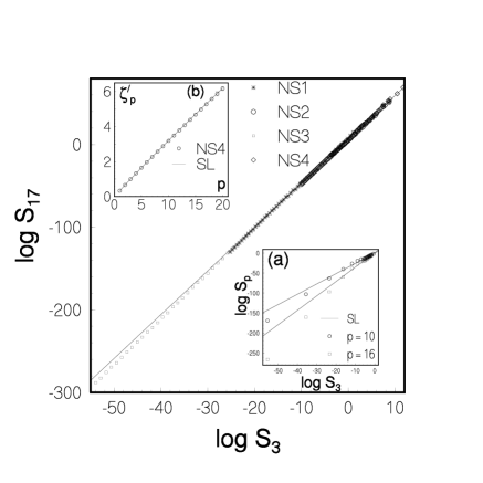
FIG. 1.: Log-log plots (base 10) of $S_{p}\/$ versus $S_{3}\/$ for $3d\/$ NS (p=17 for runs NS1-4) and GOY (run G1 in inset (a)) models showing our $k$-space ESS (Eq. 1); full lines are the SL prediction [5]. Inset (b): $\zeta_{p}^{\prime}\/$ (circles) from run NS4; the line is $\zeta_{p}^{\prime}=2(\zeta_{p}+3p/2)/11\/$, with the $\zeta_{p}=\zeta_{p}^{SL}\/$. Note the deviation of our data points from SL lines at small $S_{3}\/$, i.e., in the dissipation range.

How robust is the fair agreement of $\zeta_{p}\/$ (Fig.2) with the SL formula? Some studies [18, 19, 20] suggest that, as $Re_{\lambda}\rightarrow\infty\/$, $\delta\zeta_{p}\/\equiv(p/3-\zeta_{p})\rightarrow 0\/$. Numerical solutions of the $3d\/$ NS equation can at best achieve [8, 12, 21] $Re_{\lambda}\lesssim 220\/$, too small, by far, to resolve this issue, so we address it for the GOY model, by studying the range $4\times 10^{4}\lesssim Re_{\lambda}\lesssim 3\times 10^{6}\/$. We find (Fig.4) that $\delta\zeta_{p}$ does not vanish with increasing $Re_{\lambda}\/$; if anything, it rises marginally [22]. Systematic experimental studies at high $Re_{\lambda}\/$ are perhaps the best way to check if the trends of Fig.4 obtain in the $3d\/$ NS case.

FIG. 2.: Inertial- and dissipation-range exponents $\zeta_{p}\/$ and $\alpha_{p}\/$ (extracted from plots like Fig.1) versus $p\/$ for GOY and NS runs and their comparison with the SL formula [5] and $p/3\/$. We obtain $\zeta_{p}\/$ from our measured $\zeta_{p}^{\prime}\/$ and the formula $\zeta_{p}=11\zeta_{p}^{\prime}/2-3p/2\/$; this amplifies the error bars relative to Fig.1 [inset(b)]. Error bars for $\alpha_{p}\/$ are shown but not apparent since they are comparable to the symbol sizes.

We remark that, if we assume the hierarchy $[G_{p+1}/G_{p}]=[G_{p}/G_{p-1}]^{\gamma}\times[\lim_{p\rightarrow\infty}G_{p+1}/G_{p}]^{1-\gamma}\/$ with $\gamma^{3}=2/3\/$ (whose real-space analog is equivalent [2] to the SL moment hierarchy for the energy dissipation [5]) and use [23] $G_{p}(k)\approx C_{p}k^{\beta_{p}}\/$, we get a difference equation for $\beta_{p}\/$ identical to the SL one (our $\beta_{p}\/$ is their $-\tau_{p/3}\/$). This, when solved with the boundary conditions $\beta_{0}=\beta_{3}=0\/$ and $\lim_{p\rightarrow\infty}(\beta_{p+1}-\beta_{p})=2/9\/$, yields the SL formula (via $\zeta_{p}=-\beta_{p}+p\zeta_{3}/3\/$). However, our GESS yields $[G_{p+1}/G_{p}]\approx C^{\prime}_{p}[G_{p}/G_{p-1}]^{\Upsilon_{p}}\/$ with $\Upsilon_{p}=(\zeta_{p+1}-\zeta_{p}-1/3)/(\zeta_{p}-\zeta_{p-1}-1/3)\/$. Superficially, this might seem to violate the hierarchy assumed above, but it turns out to be consistent with our GESS form, if $\Upsilon_{p}=\gamma-2(1-\gamma)/[9(\zeta_{p}-\zeta_{p-1}-\zeta_{3})]\/$, which is precisely the SL difference equation. Of course, our GESS form can hold with $\zeta_{p}\neq\zeta_{p}^{SL}\/$; Fig. 2 shows the quality of agreement between our measured $\zeta_{p}\/$ and $\zeta_{p}^{SL}\/$.

TABLE I.: Parameters $\nu\/$ (viscosity), $\nu_{H}\/$ (hyperviscosity), $Re_{\lambda}\/$ (Taylor-microscale Reynolds number), $\tau_{e}\/$ (box-size eddy-turnover time), $\tau_{av}\/$ (averaging time), $\tau_{t}\/$ (transient time) and $k_{d}\/$ (dissipation-scale wavenumber) for our $3d\/$ NS runs NS1-4 ($k_{max}=64\/$) and GOY-model runs G1-8 ($k_{max}=2^{22}k_{0}\/$). The step size($\delta t\/$) used is 0.02 for NS1-4, $10^{-4}\/$ for G1-4, and $2\cdot 10^{-5}\/$ for G5-8.

Run	$\nu$	$\nu_{H}$	$Re_{\lambda}$	$\tau_{e}/\delta t\/$	$\tau_{t}/\tau_{e}\/$	$\tau_{av}/\tau_{e}\/$	$k_{max}/k_{d}\/$
NS1	$5\cdot 10^{-4}$	$0$	$\simeq 3.5$	$\simeq 3\cdot 10^{4}\/$	$\simeq 1\/$	$2\/$	$\simeq 4\/$
NS2	$2\cdot 10^{-4}$	$0$	$\simeq 8\/$	$\simeq 3\cdot 10^{4}\/$	$\simeq 1\/$	$\simeq 2.5\/$	$\simeq 2.3\/$
NS3	$5\cdot 10^{-4}$	$5\cdot 10^{-6}$	$\simeq 3.5$	$\simeq 3\cdot 10^{4}\/$	$\simeq 1\/$	$\simeq 1\/$	$\simeq 6.5\/$
NS4	$5\cdot 10^{-4}$	$10^{-6}$	$\simeq 22$	$\simeq 3\cdot 10^{3}\/$	$\simeq 10\/$	$\simeq 7\/$	$\simeq 2\/$
G1-4	$5\cdot 10^{-6}-10^{-7}$	$0$	$4\cdot 10^{4}-3\cdot 10^{5}$	$\simeq(1.5-2.0)10^{4}\/$	$\simeq 500\/$	$\simeq 2500\/$	$\simeq 2^{5}-2^{3}\/$
G5-8	$5\cdot 10^{-8}-10^{-9}$	$0$	$3.5\cdot 10^{5}-3\cdot 10^{6}$	$\simeq(0.7-1)10^{5}\/$	$\simeq 500\/$	$\simeq 2500\/$	$\simeq 2^{3}-1\/$

FIG. 3.: Log-log (base 10) plots of $G_{6}\/$ versus (a) $G_{15}\/$ and (b) $G_{9}\/$ illustrating our $k\/$-space GESS; (c) $H_{6,9}\/$ versus $H_{9,6}\/$ showing the universal inertial- to dissipation-range crossover (see text). The line shows the SL, inertial-range prediction.

We use a pseudospectral method [8] for our numerical solution of the incompressible $3d\/$ NS equation. We force the first two $k\/$-shells, use a box with side $L_{B}=\pi\/$ and $64^{3}\/$ modes. Our dissipation term $-(\nu+\nu_{H}k^{2})k^{2}\/$ allows for both viscosity $\nu\/$ and hyperviscosity $\nu_{H}\/$. For time integration we use an Adams-Bashforth scheme (step size $\delta t\/$) [8]. Parameters for our $3d\/$ NS runs NS1-4 are given in Table I, where $\tau_{e}\equiv L_{B}/v_{rms}\/$ is the box-size eddy-turnover time and $\tau_{av}\/$ the averaging time, after initial transients have decayed over a period $\tau_{t}\/$. We use $Re_{\lambda}\/\equiv v_{rms}\lambda/\nu\/$, where $\lambda=[\int_{0}^{\infty}E(k)dk/\int_{0}^{\infty}k^{2}E(k)dk]^{1/2}\/$, $v_{rms}=[(2/3L_{B}^{3})\int_{0}^{\infty}E(k)dk]^{1/2}\/$ and $E(k)\sim S_{2}(k)k^{2}\/$. All $S_{p}(k)\/$ are averaged over shells of radius $k\/$. Care must be exercised in choosing $\delta t\/$ and the forcing amplitude, otherwise there is a slow, but systematic, stretching of the data points along the asymptotes in Figs. 1 and 3 with increasing $\tau_{av}\/$ (over the time scales of our low-$Re_{\lambda}\/$ NS runs). Fortunately, this hardly affects our exponents: any attendant systematic errors in Fig. 2 are certainly less than the random errors indicated. Also, the agreement between our GOY and NS runs confirms our results. Our GOY-model data are, of course, of much better quality. Here Fourier components of the velocity are labeled by a discrete set of wave vectors $k_{n}=k_{0}q^{n}\/$. The dynamical variables are the complex, scalar velocities $v_{n}\/$ for each shell $n\/$; $v_{n}\/$ is affected directly only by the velocities in nearest and next-nearest shells. In spite of its simplicity, this model yields scaling properties [10, 11, 12, 13] akin to experimental ones. The GOY-model equations are:

$$\frac{d}{dt}v_{n}=iC_{n}-\nu k_{n}^{2}v_{n}+f_{n},$$ (5)

where $\nu\/$ is the kinematic viscosity, $f_{n}\/$ the external force on shell $n\/$, $C_{n}=(ak_{n}v_{n+1}v_{n+2}+bk_{n-1}v_{n-1}v_{n+1}+ck_{n-2}v_{n-1}v_{n-2})^{\ast}\/$, and $a,b,\/$ and $c\/$ can be fixed upto a constant by demanding [12], for $\nu,f_{n}=0\/$, that: $v_{n}\sim k_{n}^{-1/3}\/$ be a stationary solution of Eq.(4); and the GOY-model kinetic energy and helicity be conserved. We adopt the conventional parameters [11, 12] $k_{0}=2^{-4},\;q=2,\;a=1,\;b=c=-1/2\/$ and use $f_{n}=5\cdot 10^{-3}(1+i)\delta_{n,1},\/$ i.e., we force the first shell [24]. The GOY-model structure functions are $S_{n,p}\equiv\langle|v_{n}|^{p}\rangle\sim k_{n}^{-\zeta_{p}}\/$ [10, 11, 12]; reliable values of $\zeta_{p}\/$ obtain [12] if we use $\Sigma_{n,p}=\langle|\Im[v_{n}v_{n+1}v_{n+2}+v_{n-1}v_{n}v_{n+1}/4]|^{p/3}\rangle\/$ since this removes an underlying $3-\/$cycle. We have used $\Sigma_{n,p}\/$ to obtain Fig.4 [25], but $S_{n,p}\/$ in Figs.1-3 for consistency with $3d\/$ NS. We use an Adams-Bashforth scheme [11] (step size $\delta t\/$) to integrate Eq. (4). The average of the time scale associated with the smallest wavenumber, $(|v_{1}|k_{1})^{-1}\/$, gives the “box-size” eddy turnover time. Table I lists other parameters for our 8 GOY-model runs G1-8, for which we use (cf., [11]) $E(k)=S_{n,2}/k_{n}\/$, $\lambda=2\pi/k_{0}[\sum_{n}S_{n,2}/\sum_{n}k_{n}^{2}S_{n,2}]^{1/2}\/$, and $v_{rms}=[k_{0}\sum_{n}S_{n,2}/\pi]^{1/2}\/$. This yields $Re_{\lambda}\sim\nu^{-0.5}\/$, as expected [26] at large $Re_{\lambda}\/$.

Experimental evidence for the slope change in the dissipation range in real-space analogs of Fig.1 was given by Stolovitzky and Sreenivasan [7], who postulated ${\cal{S}}_{p}\sim{\cal{S}}_{3}^{\alpha^{\prime}_{p}}\/$ in the dissipation range and suggested $\alpha^{\prime}_{p}\simeq(\zeta_{3p/2}+p/2)/(\zeta_{9/2}+3/2)\/$. We have not been able to obtain a simple relation between our $\alpha_{p}\/$ and their $\alpha^{\prime}_{p}\/$ (unlike [14] that between $\zeta_{p}\/$ and $\zeta^{\prime}_{p}\/$) since $S_{p}\/$ does not have a power-law dependence on $k\/$ in the dissipation range. It would be very interesting to extend such experimental studies to test the universality of dissipation-range asymptotics (e.g., in different flows) and the crossover suggested here. The universal multiscaling in the dissipation range that we have elucidated is a manifestation of strongly intermittent (multifractal) dissipation which is believed to occur [16] even at low $Re_{\lambda}\/$. We believe that this multiscaling should extend far enough into the dissipation range before corrections set in because of the breakdown of (a) the incompressibility assumption (at large Mach numbers) and/or (b) hydrodynamics (at molecular length scales). Preliminary studies [27] yield similar phenomena in MHD turbulence.

FIG. 4.: Log-log plot(base 10) of $\delta\zeta_{p}\/$ versus the Taylor-microscale Reynolds number $Re_{\lambda}\/$ for our GOY runs (G1-8) with $p=6,8\ldots,20\/$ (from bottom to top). The dotted ($p=6\/$) and dashed ($p=8\/$) lines show the SL results [5]. Error bars are shown but are often smaller than the symbol sizes.

We thank S. Ramaswamy for discussions, CSIR and BRNS (India) for support, and SERC (IISc, Bangalore) for computational resources.