Winding number instability in the phase-turbulence regime of the Complex Ginzburg-Landau Equation

Abstract

We give a statistical characterization of states with nonzero winding number in the Phase Turbulence (PT) regime of the one-dimensional Complex Ginzburg-Landau equation. We find that states with winding number larger than a critical one are unstable, in the sense that they decay to states with smaller winding number. The transition from Phase to Defect Turbulence is interpreted as an ergodicity breaking transition which occurs when the range of stable winding numbers vanishes. Asymptotically stable states which are not spatio-temporally chaotic are described within the PT regime of nonzero winding number.

Spatio-temporal complex dynamics [2, 3] is one of the present focus of research in nonlinear phenomena. Much effort has been devoted to the characterization of different dynamical phases and transitions between them for model equations such as the Complex Ginzburg-Landau Equation (CGLE) [2, 4, 5, 6, 7, 8, 9, 10, 11, 12]. One of the main questions driving these studies is whether concepts brought from statistical mechanics can be useful for describing complex nonequilibrium systems [4, 13]. In this paper we give a characterization of the spatio-temporal configurations that occur in the Phase Turbulence (PT) regime of the CGLE (described below), for a finite system, in terms of a global wavenumber. This quantity plays the role of an order parameter classifying different phases. We show that in the PT regime there is an instability such that a conservation law for the global wavenumber occurs only for wavenumbers within a finite range that depends on the point in parameter space. Our study is statistical in the sense that averages over ensembles of initial conditions are used. Our results allow a characterization of the transition from PT to Defect or Amplitude Turbulence (DT) (another known dynamical regime of the CGLE) as the line in parameter space in which the range of conserved global wavenumbers shrinks to zero.

The CGLE is an amplitude equation for a complex field $A({\bf x},t)$ describing universal features of the dynamics of extended systems near a Hopf bifurcation [2, 8].

$$\partial_{t}A=A+(1+{\it i}c_{1})\nabla^{2}A-(1+{\it i}c_{2})\mid A\mid^{2}A\ .$$ (1)

Binary fluid convection [14], transversally extended lasers [15], chemical turbulence[16], bluff body wakes [17], among other systems can be described by the CGLE in the appropriate parameter range. We will restrict ourselves in this paper to the one-dimensional case, that is $A=A(x,t)$, with $x\in[0,L]$. For this situation a major step towards the analysis of phases and phase transitions in (1) was the identification [4, 5, 6] of different chaotic regimes in different regions of the parameter space $[c_{1},c_{2}]$ (see Figure 1).

FIG. 1.: Regions of the parameter $[c_{1},c_{2}]$-space for the CGLE displaying different kinds of regular and chaotic behavior. Lines $L_{1},L_{3}$ were determined in[4, 5, 6].

Eq. (1) has plane-wave solutions $A_{k}=\sqrt{1-k^{2}}e^{ikx}$ with $k\in[-1,1]$. When $c_{1}c_{2}>-1$ there is a range of wavenumbers $[-k_{E},k_{E}]$ such that the plane-wave solutions with wavenumber in this range are linearly stable. They become unstable outside this range (the Eckhaus instability [7]). The limit of this range, $k_{E}$ approaches zero as the product $c_{1}c_{2}$ approaches $-1$, so that the range of stable plane waves vanishes by approaching from below the line $c_{1}c_{2}=-1$ (the Benjamin-Feir or Newell line, labeled BF in Fig.1). Above that line no plane wave is stable and different turbulent states exist. The authors of [4, 5, 6] identified three different regimes in different regions above the BF line (Fig.1): PT, DT, and bichaos. Among these regimes, the transition between PT and DT has received special attention [4, 11, 18]. In spite of the fact that there are some indications that this transition can be ill-defined in the $L\rightarrow\infty$ limit [6, 10, 11], the PT regime is robustly observed for any finite size system and for finite observation times, with the transition to DT appearing at a quite well defined line ($L_{1}$ in Fig.1) [10]. In the DT region the modulus $|A|$ of $A=|A|e^{i\phi}$ becomes zero at some instants and places (called defects), so that the phase $\phi$ becomes undefined and the winding number $\nu\equiv\frac{1}{2\pi}\int_{0}^{L}\partial_{x}\phi dx$ changes value during evolution. In contrast, dynamics maintains the modulus of $A$ far from zero in the PT region, so that $\nu$ is thought to be a constant of motion there. A global wave number of the configuration can be defined as $k\equiv 2\pi\nu/L$. These different regimes were originally identified from the analysis of the space-time density of defects. If this picture is correct, one can speculate that the transition between DT and PT would be a kind of ergodicity breaking transition [19] as in other systems described by statistical mechanics. DT would correspond to a “disordered” phase and $\nu$ classifies different “ordered” phases in PT. However, we note that most studies of the PT regime have only considered in detail the case of $\nu=0$. In fact the phase diagram in Fig.1 was constructed for this case. In order to provide a better understanding of the PT-DT transition we undertake in this Letter a systematic study of PT configurations with $\nu\not=0$ .

Typical configurations of the PT state of zero winding number consist of pulses in $|A|$, corresponding to phase sinks, that travel and collide rather irregularly on top of a $k=0$ unstable background wave (that is, a uniform oscillation)[4, 6]. The phase of these configurations strongly resembles solutions of the Kuramoto-Shivashinsky (KS) equation. Quantitative agreement has been found between the $\nu=0$ PT states of the CGLE and solutions of the KS equation near the BF line[11]. The more obvious effect of a non-zero $\nu$ is the appearance of a uniform drift added to the irregular motion of the pulses. In addition Chaté[5, 6] reported an earlier breakdown of the PT regime when $\nu\not=0$. Our results below show that not all the winding numbers are in fact allowed in the PT region at long times. PT states with too large $|\nu|$ are only transients and decay to states within a band of allowed winding numbers. The width of this band shrinks to zero when approaching the line $L_{1}$. In addition we find that the allowed non-zero winding number states are not of a single type. We have identified three basic types of asymptotic states for $\nu\neq 0$. Two of them are different from the usually described PT states in the sense that they do not exhibit spatio-temporally chaos.

In order to study the dynamics of states with $\nu\neq 0$ we have performed simulations extensively covering the PT region of parameters of Fig. 1. Only a small part of the simulations is shown here, and the rest will be reported elsewhere. We use a pseudo-spectral code with periodic boundary conditions and second-order accuracy in time. Spatial resolution was typically 512 modes, with runs of up to 4096 modes to confirm the results. We work at fixed system size $L=512$. The initial condition in our simulation is a plane wave of the desired winding number, slightly perturbed by a white Gaussian random field. The initial evolution of the spatial power spectrum is well described by the linear stability analysis around the initial plane wave: typically the perturbation grows mostly around the most unstable wavenumbers identified from such linear analysis. After some time the system reaches a state similar to the $\nu=0$ PT, except for a non-zero average velocity of the chaotically travelling pulses. We call this state riding PT. Its spatial power spectrum is broad and unsteady, with the more active wavenumbers located around the one determined by the initial winding number. We observe that when this winding number is small, it remains constant in time, and the system either remains in the riding PT state or approaches one of the more regular asymptotic states that will be described below. If $|\nu|$ is initially too high, the competition between wavenumbers leads to phase slips that reduce $|\nu|$ until a value inside an allowed range is reached. Then the system evolves as before.

We present in Fig. 2 the temporal evolution of $\bar{\nu}(t)$, the average of $\nu(t)$ over 50 independent realizations of the random perturbation added to the initial plane wave for a fixed point in parameter space. The variance among the sample of 50 realizations is also shown. Three initial values $\nu_{i}$ of the winding number are shown. $\bar{\nu}(t)$ typically presents a decay from $\nu_{i}$ to the final winding number $\nu_{f}$.

FIG. 2.: a) Temporal evolution of $\bar{\nu}(t)$ for three different initial winding numbers $\nu_{i}=19$ (solid), $15$(dotted), $10$ (dashed) . $c_{1}=2.1,c_{2}=-0.75$. b) Winding number standard deviation $\sigma$.

The decay is found to take place in a characteristic time $\tau$ that we quantify as the time for which half of the jump in $\nu$ has been attained. Figure 3 shows $1/\tau$ for different values of $\nu_{i}$. The different curves correspond to different values of $c_{2}$ with fixed $c_{1}$. Similar results were obtained for $c_{2}$ fixed and varying $c_{1}$. $\tau$ increases with an apparent divergence as $\nu_{i}$ approaches a particular value $\nu_{c}$ which is a function of $c_{1}$ and $c_{2}$. We estimate this $\nu_{c}$ by fitting linearly the data for $1/\tau$. Other fits involving non-trivial critical exponents have been tried, but they do not improve the simpler linear one in a significant manner. A very similar value of $\nu_{c}$ is obtained by simply determining the value of $\nu_{i}$ below which $\nu(t)$ does not change in any of the realizations. Values of $\nu_{c}$ from some of the simulations are in the inset of Fig. 3. $\nu_{c}$ vanishes as $c_{2}$ approaches the transition line $L_{1}$ (or $L_{3}$ when passing through the bichaos region). For example, the linear fitting of the data in the inset of Fig.3 and extrapolation towards zero $\nu_{c}$ reproduces the value for $L_{1}$ of [4, 6] ($c_{2}\approx-0.9$ for $c_{1}=2.1$) within the fitting error in $c_{2}$ of $\pm 0.02$.

FIG. 3.: Inverse of the characteristic time for winding number relaxation as a function of the initial winding number. The value of $c_{1}$ is fixed ($c_{1}=2.1$) and $c_{2}$ varies from near the B-F line ($c_{2}=-1/2.1$) to the $L_{1}$ line ($c_{2}\approx-0.9$). Different symbols correspond to $c_{2}=-0.6$ ($+$), $c_{2}=-0.7$ ($\ast$), $c_{2}=-0.75$ ($\Diamond$), $c_{2}=-0.8$ ($\triangle$), $c_{2}=-0.83$ ($\Box$). The inset shows the critical winding number ($\nu_{c}$) as a function of $c_{2}$.

The winding number instability found here in the PT region is strikingly similar to the Eckhaus instability of travelling waves below the BF line of Fig. 1 [7]: There is a range of allowed winding numbers such that configurations outside this range undergo phase slips until an allowed $\nu$ is reached. The difference is that below the BF line, the attractor for each stable $\nu$ is a travelling plane wave of wavenumber $k$, whereas each $\nu$, or equivalent global wave number, characterizes phase turbulent attractors above the BF line. The allowed range of travelling waves shrinks to zero when $(c_{1},c_{2})$ approaches the BF from below, whereas above BF, the allowed $\nu$ range shrinks to zero when approaching the $L_{1}$ line from the right. In this picture, the transition PT-DT appears as the BF line associated to an Eckhaus-like instability for phase turbulent waves. Since the presence of chaotic fluctuations is a kind of self generated “noise” present in the system, this winding number instability should be compared to the Eckhaus instability in the presence of stochastic noise [20], rather than to the deterministic one. The comparison shows qualitative similarities between both cases, but quantitative agreement such as similar critical exponents or scaling laws has not been found. The comparison is also instructive because it can be shown that, for the one-dimensional stochastic case, there is no true long range order, and therefore no true phase transition in the infinite size limit [21]. But for finite sizes and finite observation times well defined effective transitions and even critical exponents can be introduced[20]. The PT-DT transition in the CGLE can be an effective transition of this kind. In order to further characterize the robustness of the effective transition an analysis of system size effects should be performed. Preliminary results indicate that the $\nu_{c}$ obtained for each $(c_{1},c_{2})$ point grows linearly with system size $L$, as it should happen for a well defined extensive quantity.

Finally we consider the nature of the asymptotic states allowed within the band of “stable” $\nu$.

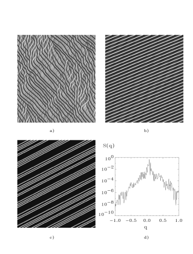
FIG. 4.: Spatiotemporal evolution of $\partial_{x}\phi(x,t)$ with time running upwards and $x$ in the horizontal direction. The lighter grey correspond to the maximum value of $\partial_{x}\phi(x,t)$ and darker to the minimum. Different scales of grey are used in each case in order to see the significant structures. a) Last $10^{2}$ time units of a run $10^{4}$ time units long for a riding PT state at $c_{1}=2.1$ , and $c_{2}=-0.83$. The initial condition was a TW with $\nu_{i}=20$ that decayed to $\nu_{f}=-1$ after a short time. b) Last $10^{2}$ time units of a run $10^{5}$ time units long for a quasiperiodic state. The initial condition is random noise with an amplitude of $0.05$. $c_{1}=2.0$ , and $c_{2}=-0.8$. c)Last $10^{2}$ time units of a run $10^{4}$ time units long for a frozen turbulence state. The initial condition is a TW of $\nu_{i}=12$ that decayed to $\nu_{f}=6$ after a short time. $c_{1}=1.75$ , and $c_{2}=-0.8$. d) Spatial power spectrum $S(q)$ as a function of wavenumber for the frozen turbulence configuration shown in c). This spectrum is constant in time.

We have numerically found three basic types of states in the PT region of parameters with non-zero $\nu$. Fig. 4 shows in gray levels the value of $\partial_{x}\phi(x,t)$ as a function of $x$ and $t$. The state shown in the top left is the familiar[6] riding PT, which is similar to the PT usually seen for $\nu=0$ (wiggling pulses in the gradient of the phase) except for a systematic drift in a direction determined by $\nu$. The other two states do not show spatio-temporal chaos. They can be described as the motion in time of a spatially rigid pattern on the top of a plane wave (with $k\neq 0$) background and with periodic boundary conditions. The state shown in the top right consists of equidistant pulses travelling uniformly. They are the quasiperiodic states described in [7]. The state shown in the bottom left, that we call frozen turbulence consists of pulses uniformly travelling on a plane wave background, as in the quasiperiodic case, but now the pulses are not equidistant from each other. The spatial power spectrum is shown for this later case. It is a broad spectrum in the sense that the inverse of its width, which gives a measure of the correlation length, is small compared with the system size. This is due to the irregular positions of the pulses. In addition the spectrum is constant in time, which makes this frozen state different from riding PT. The existence of the two states with no spatio-temporal chaos (quasiperiodic and frozen turbulence) described above can be understood by analyzing the phase equation valid near the BF instability. In the case of a non-zero $\nu$ it contains terms breaking the left-right symmetry [7, 22], and it is known as Kawahara equation [23]. Its uniformly travelling solutions are related to the rigidly propagating patterns of Fig. 1b) and c). These solutions can be analyzed with the tools of Shilnikov theory [24]. The details will be discussed elsewhere.

In addition to the pure three basic states there are configurations in which they coexist at different places of space, giving rise to a kind of intermittent configurations, some of them already observed in [5]. The main results reported here, that is the existence of an Eckhaus-like instability for phase-turbulent waves, the identification of the transition PT-DT with the vanishing of the range of stable winding numbers, and the coexistence of different kinds of PT attractors should in principle be observed in systems for which PT and DT regimes above a Hopf bifurcation are known to exist [17]. We note in addition that the experimental observation of what seems to be an Eckhaus instability for non-regular waves has been already reported in [25].

Financial support from DGYCIT (Spain) Projects PB94-1167 and PB94-1172 is acknowledged. R.M. also acknowledges partial support from the Programa de Desarrollo de las Ciencias Básicas (PEDECIBA, Uruguay), the Consejo Nacional de Investigaciones Científicas Y Técnicas (CONICYT, Uruguay) and the Programa de Cooperación con Iberoamérica (ICI, Spain).

REFERENCES

- [1] on leave from Universidad de la República (Uruguay).
- [2] M. Cross and P. Hohenberg, Rev. Mod. Phys. 65, 851 (1993), and references therein.
- [3] M. Cross and P. Hohenberg, Science 263, 1569 (1994).
- [4] B. Shraiman et al., Physica D 57, 241 (1992).
- [5] H. Chaté, Nonlinearity 7, 185 (1994).
- [6] H. Chaté, in Spatiotemporal Patterns in Nonequilibrium Complex Systems , Ed. by P.E. Cladis and P. Palffy-Muhoray (Addison-Wesley, New York, 1995).
- [7] B. Janiaud et al., Physica D 55, 269 (1992).
- [8] W. van Saarloos and P. Hohenberg, Physica D 56, 303 (1992).
- [9] D. Egolf and H. Greenside, Nature 369, 129 (1994).
- [10] H. Chaté and P. Manneville, in A Tentative Dictionary of Turbulence, edited by P. Tabeling and O. Cardoso (Plenum, New York, 1995).
- [11] D. Egolf and H. Greenside, Phys. Rev. Lett. 74, 1751 (1995).
- [12] R. Montagne, , E. Hernández-García, and M. San Miguel, Physica D (1996), to appear.
- [13] P. C. Hohenberg and B. I. Shraiman, Physica D 37, 109 (1989).
- [14] P. Kolodner, S. Slimani, N. Aubry, and R. Lima, Physica D 85, 165 (1995).
- [15] P. Coullet, L. Gil, and F. Roca, Opt. Comm. 73, 403 (1989).
- [16] Y. Kuramoto and S. Koga, Progr. Theor. Phys. Suppl. 66, 1081 (1981).
- [17] T. Leweke and M. Provansal, Phys. Rev. Lett. 72, 3174 (1994).
- [18] H. Sakaguchi, Prog. Theor. Phys. 84, 792 (1990).
- [19] R. Palmer, in Lectures in the Sciences of Complexity, Ed. by D.L. Stein (Addison-Wesley, New York, 1989).
- [20] E. Hernández-García, J. Viñals, R. Toral, and M. San Miguel, Phys. Rev. Lett. 70, 3576 (1993).
- [21] J. Viñals, E. Hernández-García, R. Toral, and M. San Miguel, Phys. Rev. A 44, 1123 (1993); E. Hernández-García, M. San Miguel, R. Toral, and J. Viñals, Physica D 61, 159 (1992).
- [22] H. Sakaguchi, Prog. Theor. Phys. 83, 169 (1990).
- [23] T. Kawahara, Phys. Rev. Lett. 51, 381 (1983).
- [24] S. Wiggins, Introduction to applied nonlinear dynamical systems and chaos (Springer, New York, 1990).
- [25] L. Pan and J. de Bruyn, Phys. Rev. E 49, 2119 (1994).