Abstract

We investigate the scattering off three nonoverlapping disks equidistantly spaced along a line in the two-dimensional plane with the radii of the outer disks equal and the radius of the inner disk varied. This system is a two-dimensional scattering analog to the double-well-potential (bound state) problem in one dimension. In both systems the symmetry splittings between symmetric and antisymmetric states or resonances, respectively, have to be traced back to tunneling effects, as semiclassically the geometrical periodic orbits have no contact with the vertical symmetry axis. We construct the leading semiclassical “creeping” orbits that are responsible for the symmetry splitting of the resonances in this system. The collinear three-disk-system is not only one of the simplest but also one of the most effective systems for detecting creeping phenomena. While in symmetrically placed $n$-disk systems creeping corrections affect the subleading resonances, they here alone determine the symmetry splitting of the 3-disk resonances in the semiclassical calculation. It should therefore be considered as a paradigm for the study of creeping effects.
PACS numbers: 03.65.Sq, 03.20.+i, 05.45.+b

Published in Phys. Rev. A 54 (1996) 2745-2754

1 Introduction

Quantum mechanics tells us that the eigenfunctions of the one-dimensional Schrödinger equation of lowest eigenvalue have no nodes, the next-lowest eigenfunctions have one node, etc.

Figure 1: Symmetric double-well potential $V(x)$ plotted (solid line) together with the corresponding single-well subpotentials (dashed lines). In addition, the classical turning points $-x_{2}$, $-x_{1}$, $x_{1}$ and $x_{2}$ at the total energy $E$ are shown and the geometrical periodic orbits (long-dashed line) as well as the tunneling orbit (short-dashed line) are indicated.

So, it is well known that the ground state of a particle in the (symmetric) double-well potential (see Fig. 1) is not centered at the bottom of one well, as one might naively infer from purely classical considerations, but instead is given by the spatially even combination of (approximately) harmonic-oscillator states centered at the bottom of the two wells, whereas the first excited state is given by the spatially odd combination. The degeneracy of the two ground-state energy eigenvalues belonging to each of the single-well potentials individually is broken in the double-well case. However, this splitting cannot result from any perturbative $\hbar$ corrections that alter the even and the odd combinations in the same way, but only from the barrier penetration. In fact, the difference between the odd and even energy combination is proportional to the barrier-penetration factor

$$e^{-\frac{1}{\hbar}\int_{-x_{1}}^{x_{1}}dx\sqrt{2m[V(x)-E]}}\;,$$ (1)

where $-x_{1}$, $x_{1}$ are the (inner) classical turning points, $V(x)$ the potential and $E$ the ground-state energy, and $m$ is the mass of the particle.

The splitting is thus inherently a nonperturbative effect linked semiclassically to tunneling orbits or instantons; see, e.g., Refs. [1, 2, 3]. This means that periodic orbit theory with only geometrical orbits cannot describe the splitting of the single-well states in even and odd double-well states, as long as the energy is below the potential barrier. Periodic orbits with tunneling sections have to be added to the semiclassical theory. The reason is that as long as the energy is below the potential barrier the geometrical orbits can never reach the symmetry axis of the double-well potential at $x=0$ and therefore are not sensitive to the boundary condition (Neumann or Dirichlet) chosen there.

Here we want to construct the simplest two-dimensional and scattering analog of the double-well-potential problem. It consists of three nonoverlapping disks centered and equally spaced on a straight line in the two-dimensional plane, where the outer disks have the same radius, whereas the radius of the inner disk is free to vary [see Fig. 2(a)].

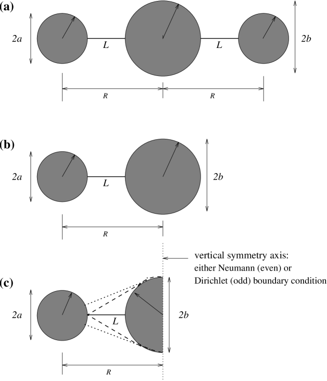
Figure 2: (a) Collinear three-disk system in the full domain. The outer disks have a radius of size $a$, whereas $b$ is the radius of the inner disk. The center-to-center separation $R$ and the length $2L$ of the geometrical periodic orbit (thin solid line) are related as $L=R-a-b$. (b) The corresponding two-disk (sub)system in the full domain. (c) The half-symmetry reduced collinear three-disk system in the half domain. In addition, the vertical symmetry axis is shown and the leading creeping periodic orbits are indicated by dotted and dashed lines.

The analog of the single-well potential is the two-disk subset of the upper problem consisting of one of the original outer disks and the middle disk, where the radii as well as the distances of the disks are kept unaltered [see Fig. 2(b)]. As in the double-well potential, the geometrical periodic orbits never hit the vertical symmetry axis, which goes through the center of the middle disk perpendicular to the horizontal symmetry axis (the latter is in turn given by the line through the centers of the three disks); see Fig. 2(c). The splitting can only come from nongeometrical periodic orbits. In fact, only creeping periodic orbits are left over for this purpose (see Refs. [4, 5, 6, 7, 8], based on Refs. [9, 10]). These simple phenomena should not be mixed up with the chaos-assisted tunneling of Refs. [11, 12] or the geometrical interpretation of multidimensional tunneling for bound state systems of Refs. [13, 14].

In Sec. 2 we will describe the collinear three-disk system in more detail and in Sec. 3 we outline the calculation (details can be found in the Appendix) and give results. Conclusions are given in Sec. 4.

2 Collinear three-disk system

The standard three-disk system with its three equally sized and nonoverlapping disks centered at the corners of an equilateral triangle in the two-dimensional plane is discussed in the literature [15, 16, 17, 18, 19, 20, 21] as one of the simplest (if not the simplest) classically completely chaotic scattering system. Here we consider a different three-disk system with the centers of the three disks arranged in equal intervals on a straight line, where the outer disks have equal radii $a$, whereas the radius $b$ of the inner disk is free to vary; see Fig. 2(a). As the original three-disk system is the paradigm for a chaotic scattering system, the new collinear three-disk system can be taken as the paradigm for scattering system with maximal creeping corrections.

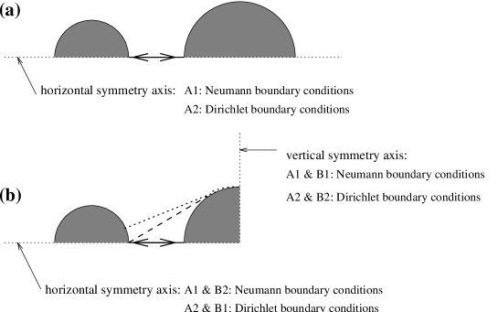
Figure 3: (a) Two-disk (sub)system in its fundamental domain. (b) Collinear three-disk system in its fundamental domain. Indicated are the geometrical periodic orbits (solid lines) and the leading creeping periodic orbits (dashed and dotted lines). In addition, the irreducible $C_{2}$ and $C_{2v}$ representations of the two- and three-disk system, respectively, and the corresponding boundary conditions on the horizontal and vertical symmetry axes are shown.

Note that the collinear three-disk system is invariant under reflections with respect to the horizontal symmetry axis (defined by the centers of the three disks) and – as long as the outer disks are of the same radius and the spacings between the disks are equal – with respect to the vertical symmetry axis (which goes through the center of the middle disk, perpendicular to the horizontal symmetry axis). Thus the states and resonances of the collinear three-disk system can be classified according to the four irreducible representations of the the $C_{2v}$ group, whereas each of the two-disk subsystems in general only has a $\sigma_{h}$ reflection symmetry with respect to its horizontal symmetry axis (as the radii of the two disks can be different). As usual, it is easier to study the quantum mechanics and semiclassics of these systems desymmetrized in the fundamental domain, instead of the original systems in the full region. The fundamental region of the collinear three-disk system is only one quarter of the full region, bounded by the horizontal and vertical symmetry axis – see Fig. 3(b). The totally symmetric $A_{1}$ $C_{2v}$-representation is characterized by even or Neumann boundary conditions for the wave functions on the horizontal and vertical symmetry axis, whereas the totally antisymmetric $A_{2}$ representation has just the opposite transformation behavior, i.e., the boundary conditions are both of the Dirichlet type. In addition, there exist two more irreducible representations of mixed symmetry, the $B_{1}$ and $B_{2}$ representation; the former transforms symmetrically with respect to the vertical symmetry axis and antisymmetrically with the respect to the horizontal one and the $B_{2}$ representation has the opposite transformation properties. The two-disk subsystems have only two irreducible $C_{1h}$ ($\cong$ $C_{1v}$ $\cong$ $C_{s}$) representations: the totally symmetric $A^{\prime}$ one, which is even with respect to reflections off the horizontal symmetry axis, whereas the states of the totally antisymmetric $A^{\prime\prime}$ representation have an “odd” transformation law. In the following we will use the nonstandard notation $A_{1}$ ($A_{2}$) instead of the standard on $A^{\prime}$ ($A^{\prime\prime}$) for the $C_{1h}$ representations; see, e.g., Ref.[22]. The fundamental region of the two-disk subset is therefore the half plane with respect to the horizontal symmetry axis; see Fig. 3(a).

Note that the collinear three-disk system possesses only two geometrical periodic orbits in the full domain. They are symmetric with respect to the vertical symmetry axis and therefore map into only one geometrical periodic orbit in the fundamental domain [see Figs. 2(a) and 3(b)]. It runs along the horizontal symmetry axis and should therefore be treated as a boundary orbit (see Refs. [23, 24] for a discussion of boundary orbits). The same is true for the solely existing boundary orbit of the two-disk subsystem, which also runs along the horizontal symmetry axis. This means that the contributions of the geometrical orbit to the $B_{1}$ and $A_{2}$ states and resonances of the collinear three-disk system and to the $A_{2}$ resonances and states of the two-disk subsystems are strongly suppressed [see Eq.(A7) of the Appendix].

As the symmetries with respect to the horizontal symmetry axis are common for the collinear three-disk system and its two-disk subsystems, they are not essential for our discussion. Instead of working with the full three-disk-system, one could as well only consider it in the half domain defined by its horizontal symmetry axis [not by its vertical one as in Fig. 2(c)], and compare it to the two-disk subsystem in the fundamental domain [Fig. 3(a)]. By choosing either Neumann or Dirichlet boundary conditions on the horizontal symmetry axis of these system one can then enhance or suppress the geometrical relative to the creeping contributions. So in an experimental billiard setup, one could work with half disks (instead of full disks) that are aligned at the reflecting boundary of an otherwise “open” billiard geometry; see, e.g., Ref. [25]. To our knowledge this reference contains the only known experiment on the scalar open n-disk scattering problem. It is done with microwaves in a cavity with absorbing outside walls. As long as the extension in the third direction (perpendicular to the quasi-two-dimensional n-disk setup that is experimentally realized with reflecting metal cylinders) is so small that only the lowest mode is excited in that direction, the stationary electromagnetic problem is mathematically equivalent to the stationary two-dimensional quantum (scattering) problem of a point-particle. In that respect this experiment as well as any possible extension to the collinear three-disk setup serves just as an “analog computer” to our digitally computed data.

The analog of the original one-dimensional double-well potential is the partially desymmetrized collinear three-disk system in its half domain relative to its horizontal symmetry axis and the analog of the two single-well potentials are the two two-disk subsystems in the fundamental region. The single-well eigenfunctions correspond to the $A_{1}$ (or $A_{2}$) states of the two-disk subsystems, and the even and odd combinations of the single-well functions to the $A_{1}$ and $B_{2}$ (or $B_{1}$ and $A_{2}$) states of the collinear three-disk system in its fundamental domain [Fig. 3(b)]. The correspondence of the geometrical orbits is obvious. In the double well as in the collinear three-disk system the geometrical orbits do not reach the “$x$=0 axis” or the corresponding vertical symmetry axis, respectively. They cannot produce the symmetry splitting. The role of the tunneling orbit in the double-well potential is taken over by those creeping orbits of the three-disk system that reach the vertical symmetry axis [see, e.g., Figs. 2(c) and 3(b)] as only those orbits can produce the symmetry splitting of the $A_{1}$ ($A_{2}$) two-disk resonances into the $A_{1}$ and $B_{2}$ ($B_{1}$ and $A_{2}$) three-disk resonances, corresponding to the splitting of the single-well eigenenergies into the even and odd double-well eigenenergies. However, whereas in the double-well problem the tunneling corrections scale exponentially with $\hbar^{-1}$, the creeping corrections along a circular path scale exponentially with $\hbar^{-{1\over 3}}$ [9, 10]. Common to both is the nonperturbative structure. In detail, the creeping tunneling exponent of mode number $\ell=1,2,3,\dots$ is given as [10, 6]

$$\alpha_{\ell}(s,p)=q_{\ell}e^{-i\frac{\pi}{6}}\left(\frac{p}{6\hbar\rho(s)^{2}}\right)^{1\over 3}\ .$$ (2)

Here $p$ is the momentum, $\rho(s)$ is the local radius of curvature of the creeping path (which parametrically depends on the length $s$ of the creeping arc), and $q_{\ell}$ (with $\ell=1,2,3,\dots$) is the $\ell^{\,\rm th}$ zero of the Airy integral $A(q)=\int_{0}^{\infty}dt\,\cos(tq-t^{3})$ which can be approximated as

$$q_{\ell}\approx{{1\over 2}}6^{1\over 3}\left[3\pi\left(\ell-{{1\over 4}}\right)\right]^{{2\over 3}}\ .$$ (3)

If $x_{a}$ and $x_{b}$ are the start and end points of the creeping section, the semiclassical creeping Green’s function reads [6]

$$G_{\ell}^{D}(x_{a},x_{b},p)=e^{-\int_{0}^{s}ds^{\prime}\,\alpha(s^{\prime},p)}e^{\frac{i}{\hbar}S(x_{a},x_{b},p)}\;,$$ (4)

where $s$ is the length of the creeping arc from the point $x_{a}$ to the point $x_{b}$ and $S(x_{a},x_{b},p)$ is the action along it. For the special case that the creeping arc is of circular shape of radius $a$ with an arc angle $\delta\phi$, the formula (4) then simplifies to

$$G_{\ell}^{D}(\delta\phi,p)=\exp\left({-q_{\ell}e^{-i\pi/6}\left(\frac{pa}{6\hbar}\right)^{1\over 3}\delta\phi}\right)\exp\left({\frac{i}{\hbar}pa\delta\phi}\right)\;,$$ (5)

such that the nonperturbative creeping contribution can be read off easily. Note that the exponent of the (leading) creeping “tunneling” suppression factor $\exp[-q_{1}\cos(\pi/6)(ka/6)^{1\over 3}\delta\phi]$ (where $k$ is the wave number) scales linearly with the creeping angle and only as third root of the creeping radius. Thus the creeping suppression is governed by the creeping angle and the size of the disk is only of secondary importance. We will observe this fact in the comparison of the exact to the semiclassical data (see also the discussion at the end of the Appendix). Note further that the creeping is suppressed with increasing wave number $k$, such that the splitting eventually vanishes in the semiclassical limit ${\rm Re}\,k\to\infty$.

3 Calculation and results

In this section the quantum-mechanical and semiclassical calculations are briefly explained (details can be found in the Appendix) and finally results for the splitting of the two-disk resonances into the resonances of the collinear three-disk system are shown.

As the collinear three-disk system and the two-disk subsystems involve disks of different sizes, the quantum-mechanical calculation of Ref. [18] has to be generalized. This was done in Ref. [26], where in fact the characteristic determinant ${\rm det}{\bf M}(k)$ of any $n$-disk system involving $n<\infty$ nonoverlapping disks of any sizes has been constructed (see the Appendix). The zeros in the lower complex wave-number ($k$) plane of this Korringa-Kohn-Rostoker-type [27, 28] determinant define the genuine multidisk scattering resonances [18, 26]. The fact that the collinear three-disk system and its subsystems have disks of two different sizes implies that the corresponding characteristic matrices ${\bf M}(k)$, even in its desymmetrized form, cannot just be expanded in the angular momentum eigenbasis $\{|\,l\,\rangle\}$ of one disk alone, but have to be expanded in the so-called superbasis $\{|j,l\rangle\}$, which acts on the disk surface sections $j$ in the fundamental domain [26] (see also the Appendix). Thus the cumulant expansion of the characteristic determinants (see Refs. [4, 5, 26]) is effectively not organized in terms of the first cumulant ${\rm Tr}{\bf A}(k)$ [where ${\bf A}(k)\equiv{\bf M}(k)-{\bf 1}$ is the trace-class kernel [26]], but in terms of the second and higher cumulants, e.g., ${{1\over 2}}\{({\rm Tr}{\bf A}(k))^{2}-{\rm Tr}{\bf A}^{2}(k)\}$, etc. The semiclassical contribution of the first cumulant in the desymmetrized collinear three-disk system in fact corresponds to a ghost orbit (see, e.g., Refs. [29, 28]) between the outer two disks, which is obstructed by the presence of the middle disk. All the “nonghost” geometrical and creeping periodic orbits of the collinear three-disk system and its two-disk subsystems have therefore an even topological length and especially the shortest orbits in the fundamental domain are already of topological length 2. From the semiclassical point of view of Refs. [4, 5] this is obvious as the orbits have an even number of contacts (in the sense of specular reflections for geometrical legs and tangential creeping for creeping legs) with the disks. The number of these contacts corresponds just to the power $m$ in the trace ${\rm Tr}{\bf A}^{m}(k)$, as the $m^{\,\rm th}$ trace involves $m$ sums. In the semiclassical calculation, each of these $m$ sums are replaced either by an integration and a following saddle point approximation (which corresponds to a specular reflection) or by a sum over the creeping poles (which corresponds to a creeping contact).

As with increasing topological order the number of creeping orbits is increasing dramatically and as, on the other hand, the leading creeping orbits give the dominant contribution to the splitting of the resonances, we show only semiclassical results for the lowest topological order, namely order 2. This corresponds to the curvature expansion [30, 31] of the Gutzwiller-Voros zeta function [32, 33] up to this topological order [see Eqs.(A14) and (A15) of the Appendix]. For a qualitative comparison to the exact data this is more than sufficient.

In Figs. 4 and 5 the exact collinear three-disk $A_{1}$ and $B_{2}$ resonances (plotted both as diamonds) are compared with the exact $A_{1}$ resonances of the two-disk subsystem (plotted as crosses). The splitting in the imaginary part is clear from the figures. The splitting in the real part is of similar size, but compressed in the figures because of the different scales used for the real and imaginary $k$-axes. In addition, the predictions of the geometrical orbit [see (A7) and (A15)] are plotted (as boxes), which describes very well the leading resonances of the two-disk subsystem, with more and more accuracy for larger and larger ${\rm Re}\,k$. The deviations between the exact quantum-mechanical data and the semiclassical predictions which are visible in Figs. 4–8 for small wave numbers result, in the case ${\rm Rek}{\mbox{\raisebox{-2.58334pt}{$\,{\stackrel{{\scriptstyle>}}{{\sim}}}\,$}}}1/a$, from the neglect of $\hbar$ corrections [34, 35, 36], subleading creeping orbits (see the discussion at the end of the Appendix) and subleading terms in the Airy expansion of the creeping propagators [37, 38]. The deviations for ${\rm Re}\,k\ll 1/a$ can be traced back to a breakdown of the standard semiclassical expansion in terms of geometrical and creeping orbits altogether. In that wave-number regime the quantum-mechanical wave cannot resolve the scattering obstacles, so that the semiclassical expansion has to be expressed in terms of diffractional orbits scattered from point-like centers; see Ref. [39].

Figure 4: Exact quantum-mechanical ($A_{1}$ and $B_{2}$) resonances of the collinear three-disk system (with $b=1.5a$ and $L=4a$) shown as diamonds in the complex wave-number ($k$) plane and the $A_{1}$ resonances of the corresponding two-disk subsystem are denoted by crosses. The predictions of the geometrical orbit [Eqs.(A7) and (A15)] are presented by boxes. The real and imaginary parts of $k$ are measured in units of $1/a$. Note the different scales for the real and imaginary $k$ axes.

Figure 5: Same as in Fig. 4, however, with $b=3a$.

In Figs. 6 and 7 the $A_{1}$ and $B_{2}$ resonances of the collinear three-disk system are compared with the semiclassical calculation (A14) based on the geometrical orbit (A7) and leading creeping corrections (A11) and (A12). The creeping terms reproduce, at least qualitatively, the trend of the data, i.e., the tunneling splitting between the $A_{1}$ and $B_{2}$ resonances of leading order. The subleading $A_{1}$ and $B_{2}$ resonances are of course not reproduced, as they are determined by higher-order contributions (geometrical plus creeping ones) in the curvature expansion [30, 31] of the semiclassical Gutzwiller-Voros zeta function [32, 33]. Furthermore, the stronger deviations for the low lying resonances (i.e., the systematical underestimation of the magnitude of the imaginary part) can be explained by the neglect of higher correction terms (beyond those discussed in Ref. [6]) in the Airy expansion of the creeping propagators; see, e.g., Ref. [37] for Airy correction terms in the one-disk scattering system and [38] for results in the two-disk system.

Figure 6: Exact quantum-mechanical ($A_{1}$ and $B_{2}$) resonances of the collinear three-disk system (with $b=1.5a$ and $L=4a$) shown as diamonds and boxes, respectively, in the complex wave-number ($k$) plane. The corresponding semiclassical results of Eq.(A14), which include the two leading creeping orbits, are shown as upright and diagonal crosses, respectively. The real and imaginary parts of $k$ are measured in units of $1/a$. Note the different scales for the real and imaginary $k$ axes.

Figure 7: Same as in Fig. 6, however, with $b=3a$.

Finally, in Fig. 8 the exact quantum-mechanical $A_{2}$ and $B_{1}$ resonances of the collinear three-disk system are compared with the corresponding semiclassical predictions calculated from Eq.(A14). Furthermore, the exact $A_{2}$ resonances of the two-disk subsystems are shown together with the semiclassical prediction from Eq.(A15), which involves only the geometrical orbit. By comparing these resonances with Figs. 4 and 6 (which describe the $A_{1}$ and $B_{2}$ three-disk and $A_{1}$ two-disk resonances) one can learn that the resonances of Fig. 8 are suppressed. This result is expected, as the geometrical orbit now runs on a Dirichlet line that bounds the fundamental domain (of the collinear three-disk as well as the two-disk system), such that the wave function goes to zero there, whereas before the geometrical orbit was affected by the Neumann condition. Note that the two-disk resonances are again quite well approximated (with increasing ${\rm Re}\,k$) by the predictions of the geometrical orbit alone. (The agreement is worse than in Figs. 6 and 7 as the resonances here are stronger suppressed to begin with, such that neglected subleading effects are of relative higher importance. In fact, most of the deviations should be traced back to the neglected creeping orbits of the two-disk system; see, e.g., Ref. [7] for the discussion of the similar $B_{1}$ resonances of the symmetric two-disk system.)  However, the inclusion of the creeping orbits in the semiclassical calculation is necessary in order to predict the qualitative trend of the exact three-disk data. Furthermore, one can learn from these data that the creeping orbits are now not only leading in the splitting, but in fact they even dominate the geometrical orbit in the determination of the absolute position of the resonances. This is, of course, again a consequence of the Dirichlet choice for the boundary condition on the horizontal symmetry axis, which suppresses the geometrical contributions relative to the creeping ones. In the case where one wants to maximize the creeping effects, the Dirichlet choice for the boundary condition on the horizontal symmetry axis is advantageous. However, one should note that this choice suppresses the resonances altogether, such that the Neumann choice might be still better from the phenomenological point of view, as the resonances can be more easily identified. By positioning two receiving antennas symmetrically to the horizontal symmetry axis the even and odd states with respect to that axis can be extracted experimentally. The “antennas” refer of course to the electromagnetic two-dimensional analog case (see, e.g., Ref. [25]) of the quantum scattering problem in two dimensions. By adding another pair of antennas symmetrically to the vertical symmetry axis, the remaining symmetries can be determined.

Figure 8: Exact quantum-mechanical ($A_{2}$ and $B_{1}$) resonances of the collinear three-disk system (with $b=1.5a$ and $L=4a$) shown as diamonds and boxes, respectively, in the complex wave-number ($k$) plane. The corresponding semiclassical results of Eq.(A14), which include the two leading creeping orbits, are shown as upright and diagonal crosses, respectively. Furthermore, the exact $A_{2}$ resonances of the two-disk subsystem are plotted as triangles and the corresponding semiclassical predictions based solely on the geometrical orbit [see Eq.(A15)] as stars. The real and imaginary parts of $k$ are measured in units of $1/a$. Note the different scales for the real and imaginary $k$ axes.

4 Conclusions

We have shown that the collinear three-disk system is a two-dimensional scattering analog (probably one of the simplest) of the one-dimensional two-potential bound-state problem. As in the latter case, nonperturbative contributions are needed in order to describe the splitting of the resonances (states) of the subsystems (the two-disk or one-potential problems, respectively) into the corresponding quantities of the full system. Whereas in the two-potential problem these nonperturbative contributions are given semiclassically by tunneling paths, in the collinear three-disk scattering system their role is taken over by creeping orbits, which alone determine the splitting phenomena. In the description of the leading resonances of the collinear three-disk system they are at least as important as the geometrical orbit. In the case where the Dirichlet boundary condition has been specified on the horizontal symmetry axis the creeping orbits even dominate the geometrical orbit. Thus the creeping orbits of the collinear three-disk system are of “leading nature”. This is the main qualitative difference to the standard two– and three–disk systems with symmetrically arranged disks, as there the creeping terms are inessential for the description of the leading band of resonances and do only play an important role in the case of subleading bands. In summary, the collinear three-disk system is probably the simplest (higher than one-dimensional) scattering analog of the two-potential bound-state problem and the simplest disk-scattering problem with leading creeping terms. In the same way as the standard two-disk problem is the paradigm for hyperbolic scattering systems and the standard equitriangular three-disk system is the paradigm for chaotic scattering systems, the collinear three-disk system should be considered as a paradigm for the study of creeping effects.

By replacing the disks in the collinear three-disk system by three-dimensional balls, one can easily construct a three-dimensional scattering analog system to the double-well potential problem. As in the two-dimensional collinear three-disk case, the splitting of the resonances (with respect to the vertical symmetry plane) again has to be traced back to the creeping orbits.

As mentioned in Sec. 3, the geometrical orbit spanned by the outer two disks is shadowed by the presence of the middle disk and is therefore only a ghost orbit [29, 28]. This ghost orbit can be tested in a modified three-disk array, where the middle disk is positioned off the horizontal symmetry axis along the vertical one. If the middle disk does not overlap the old center of the collinear three-disk system, the ghost orbit in fact splits into the sum of a direct geometrical orbit that is spanned by the outer disks and a geometrical orbit that, in addition, encounters a specular reflection from the middle disk. By sliding the middle disk back into its old position, one can check how and when exactly the two geometrical orbits become a ghost orbit (see, e.g., Ref.[40] for the introduction of glancing orbits [41] into periodic orbit theory). This phenomenon is strongest if the middle disk possesses Neumann boundary conditions, as then the two geometrical orbits interfere constructively, whereas they interfere destructively in the case of Dirichlet boundary conditions. In this respect a very interesting system would be a nonoverlapping four-disk system with the centers of three equally sized disks at the corners of an equilateral triangle, whereas the fourth disk (again with Neumann boundary conditions) is positioned at the center of this triangle. If the size of this fourth disk is varied, geometrical orbits can be turned into ghost orbits or vice versa. Furthermore, if the fourth disk is large enough, again only creeping orbits are left over for producing the splitting of the resonances of the three two-disk subsystems (consisting of one outer disk and the middle disk and classified according to the point-symmetry group $C_{1h}$) into the resonances of this new four-disk system, which are classified according to the point-symmetry group $C_{3v}$. Whereas the collinear three-disk system is classically hyperbolic, but nonchaotic (as its two-disk subsystems), the new four-disk system is classically completely hyperbolic and chaotic if the middle disk is small enough. By varying the ratio of the size of this fourth disk relative to the common size of the other three, one has the possibility to study the transition from an nonchaotic to a chaotic system classically, semiclassically and quantum mechanically. In the case where the boundary conditions on the fourth disk are also of Dirichlet nature, the formulas of Ref. [26] suffice to attack the quantum mechanics of the problem. Again three-dimensional generalizations are easy to generate, e.g., the four-ball analog system or, even more interesting, a (nonoverlapping) five-ball system in tetrahedral form, where four balls are positioned at the corners and the fifth in the middle.

All these suggested systems can also serve as a higher-dimensional scattering analog of the double-well potential. Still, the collinear three-disk system is by far the simplest.

Appendix A Appendix

The characteristic $n$-disk matrix ${\bf M}$ of Ref. [26] reads, in the full $n$-disk domain,

$${\bf M}_{ll^{\prime}}^{jj^{\prime}}=\delta^{jj^{\prime}}\delta_{ll^{\prime}}+(1-\delta^{jj^{\prime}})\frac{a_{j}J_{l}(ka_{j})}{a_{j^{\prime}}H_{l^{\prime}}^{(1)}(ka_{j^{\prime}})}H_{l-l^{\prime}}^{(1)}(kR_{jj^{\prime}})e^{i(l\alpha_{j^{\prime}j}-l^{\prime}\alpha_{jj^{\prime}})}(-1)^{l^{\prime}},$$ (A1)

where $-\infty<l,l^{\prime}<+\infty$ are the angular momentum quantum numbers in two dimensions, $j,j^{\prime}$ label the disks, the $J_{l}(kr)$’s are ordinary Bessel functions, and the $H_{l}^{(1)}(kr)$’s the corresponding Hankel functions of first kind. The quantity $a_{j}$ is the radius of disk $j$, $R_{jj^{\prime}}$ is the distance between the centers of disks $j$ and $j^{\prime}$, and $\alpha_{j^{\prime}j}$ is the angle of a ray from the center of disk $j$ to the center of disk $j^{\prime}$ as measured in the local (body-fixed) coordinate system of disk $j$. These quantities take the following values for the collinear three-disk systems: $j=1,2$ labels the outer disks on the right and left side, respectively, whereas $j=0$ is reserved for the inner disk. Furthermore, we have

$$a_{2} = a_{1}\equiv a\;,$$

$$a_{0} \equiv b\;,$$

$$R_{01} = R_{10}=R_{20}=R_{02}=R\;,$$

$$R_{12} = R_{21}=2R\;,$$

$$\alpha_{21} = \alpha_{12}=\pi\;,$$

$$\alpha_{20} = \alpha_{02}=\pi\;,$$

$$\alpha_{01} = \pi\quad{\rm but}\ \ \alpha_{10}=0.$$ (A2)

The characteristic matrix ${\bf M}$ of the two-disk (sub)system is of course a special case of the above, namely either $j=0,2$ or $j=0,1$.

The corresponding desymmetrized $\widetilde{\bf M}$ matrix of the collinear three-disk system in the fundamental domain reads

$${\widetilde{\bf M}}^{00}_{ll^{\prime}}[IJ]\!\! = \!\!\delta_{ll^{\prime}}\frac{1+(-1)^{I+J}\delta_{l0}}{1+\delta_{l0}}\,\left(\frac{1+(-1)^{I+1+l}}{2}\right)^{2}\;,$$

$${\widetilde{\bf M}}^{01}_{ll^{\prime}}[IJ]\!\! = \!\!\frac{\sqrt{2}}{\sqrt{(\mbox{1+$\delta_{l0}$})(\mbox{1+$\delta_{l^{\prime}0}$})}}\,\frac{\mbox{1+$(-1)^{I+1+l}$}}{2}\frac{b}{a}\frac{J_{l}(kb)}{H_{l^{\prime}}^{(1)}(ka)}\left[H_{l-l^{\prime}}^{(1)}(kR)\mbox{+}(-1)^{I+J+l^{\prime}}H_{l+l^{\prime}}^{(1)}(kR)\right],$$

$${\widetilde{\bf M}}^{10}_{ll^{\prime}}[IJ]\!\! = \!\!\frac{(-1)^{l+l^{\prime}}\sqrt{2}}{\sqrt{(\mbox{1+$\delta_{l0}$})(\mbox{1+$\delta_{l^{\prime}0}$})}}\,\frac{\mbox{1+$(-1)^{I+1+l^{\prime}}$}}{2}\frac{a}{b}\frac{J_{l}(ka)}{H_{l^{\prime}}^{(1)}(kb)}\left[H_{l-l^{\prime}}^{(1)}(kR)\mbox{+}(-1)^{I+J+l^{\prime}}H_{l+l^{\prime}}^{(1)}(kR)\right],$$

$${\widetilde{\bf M}}^{11}_{ll^{\prime}}[IJ]\!\! = \!\!\delta_{ll^{\prime}}\frac{\mbox{1+$(-1)^{I+J}\delta_{l0}$}}{\mbox{1+$\delta_{l0}$}}$$ (A3)

$$\mbox{}+\frac{(-1)^{I+1+l}}{\sqrt{(\mbox{1+$\delta_{l0}$})(\mbox{1+$\delta_{l^{\prime}0}$})}}\frac{J_{l}(ka)}{H_{l^{\prime}}^{(1)}(ka)}\left[H_{l-l^{\prime}}^{(1)}(2kR)\mbox{+}(-1)^{I+J+l^{\prime}}H_{l+l^{\prime}}^{(1)}(2kR)\right]\;,$$

with $0\leq l,l^{\prime}<\infty$ and where the indices $I$ and $J$ specify the irreducible $C_{2v}$ representations with the following identification: $I=1,2$ for the $A_{J}$, $B_{J}$ representations, respectively; i.e., $(-1)^{J+1}$ is the phase under reflection off the vertical symmetry axis and $(-1)^{I+1}$ is the phase under point reflection with respect to the center of the 3-disk system.

The characteristic matrix of the desymmetrized two-disk subsystem in the fundamental domain reads

$${\widetilde{\bf M}}^{00}_{ll^{\prime}}[K] = \delta_{ll^{\prime}}\,\frac{1+(-1)^{K+1}\delta_{l0}}{1+\delta_{l0}}\;,$$

$${\widetilde{\bf M}}^{01}_{ll^{\prime}}[K] = \frac{1}{\sqrt{(1+\delta_{l0})(1+\delta_{l^{\prime}0})}}\,\frac{b}{a}\frac{J_{l}(kb)}{H_{l^{\prime}}^{(1)}(ka)}\left[H_{l-l^{\prime}}^{(1)}(kR)+(-1)^{K+1+l^{\prime}}H_{l+l^{\prime}}^{(1)}(kR)\right]\;,$$

$${\widetilde{\bf M}}^{10}_{ll^{\prime}}[K] = \frac{(-1)^{l+l^{\prime}}}{\sqrt{(1+\delta_{l0})(1+\delta_{l^{\prime}0})}}\,\frac{a}{b}\frac{J_{l}(ka)}{H_{l^{\prime}}^{(1)}(kb)}\left[H_{l-l^{\prime}}^{(1)}(kR)+(-1)^{K+1+l^{\prime}}H_{l+l^{\prime}}^{(1)}(kR)\right]\;,$$

$${\widetilde{\bf M}}^{11}_{ll^{\prime}}[K] = \delta_{ll^{\prime}}\,\frac{1+(-1)^{K+1}\delta_{l0}}{1+\delta_{l0}}\;,$$

with $0\leq l,l^{\prime}<\infty$ and where the index $K=1,2$ refers to the irreducible $A_{K}$ representation of the point-symmetry group $C_{1h}$. More specifically, $(-1)^{K+1}=(-1)^{I+J}$ is the phase of the two-disk and three-disk states under reflection off the horizontal symmetry axis. Finally, the resonances $k_{\rm res}$ are determined as the zeros of the desymmetrized characteristic determinant [evaluated in the superspace, $\{|j,l\rangle\}$ with $j$=0,1 and $0\leq l<\infty$, acting on the disk surfaces (see Figs. 3) of the fundamental domain] in the (lower) complex wave-number ($k$) plane

$$\left\{{\rm det}{\widetilde{\bf M}}[IJ](k)\right\}_{k=k_{\rm res}}=0$$ (A5)

in the collinear three-disk case and

$$\left\{{\rm det}{\widetilde{\bf M}}[K](k)\right\}_{k=k_{\rm res}}=0$$ (A6)

in the case of the two-disk subsystems.

The fundamental geometrical orbit that is of topological length 2 and that is common to the collinear three-disk system as well as to its two-disk subsystem is given by

$$t_{\rm G}(k;K)=\frac{e^{i2Lk}}{\sqrt{|\Lambda|}\Lambda^{K-1}\left(1-\frac{1}{\Lambda^{2}}\right)}\;,$$ (A7)

where the index $K=1,2$ has been defined above. Thus the $K=2$ representations, namely, the $A_{2}$ two-disk representation and the $A_{2}$ and $B_{1}$ three-disk representations, are suppressed relatively to the $K=1$ representations, namely, the $A_{1}$ two-disk one and the $A_{1}$ and $B_{2}$ three-disk representations. This is intuitively clear as the geometrical orbit is a boundary orbit on the horizontal symmetry axis and therefore sensitive to the choice of the boundary condition for the wave function, i.e., either Dirichlet or Neumann boundary conditions; see Refs. [23, 24]. The length $2L$ of the geometrical orbit is given by

$$2L=2(R-a-b)\;,$$ (A8)

where $a$ and $b$ are the radii of the outer and inner disk, respectively, and $R$ is the center-to-center separation between these disks. The quantity $\Lambda$ is the leading eigenvalue

$$\Lambda=1+\left(1+\sqrt{1+\frac{ab}{RL}}\,\right)\frac{2RL}{ab}\$$ (A9)

of the stability matrix, which in turn is given by the product of four submatrices: a translational one from the inner to the outer disk, then a reflectional matrix linked to the outer disk, then again a translational one from the outer to the inner disk, and finally again a reflectional matrix acting at the inner disk

$$\left(\begin{array}[]{cc}{1}&{0}\\ {L}&{1}\end{array}\right)\left(\begin{array}[]{cc}{-1}&{-2/a}\\ {0}&{-1}\end{array}\right)\left(\begin{array}[]{cc}{1}&{0}\\ {L}&{1}\end{array}\right)\left(\begin{array}[]{cc}{-1}&{-2/b}\\ {0}&{-1}\end{array}\right)$$ (A10)

(see Ref. [21] for further details). Note that the reflection angle $\theta$ is zero for the two reflections, such that the off-diagonal elements $2/[\rho_{i}\cos(\theta)]$ of the reflection matrices simplify to $2/\rho_{i}$ where $\rho_{i}$ is the local radius of curvature. As there are two reflections and as the geometrical orbit does not touch the vertical symmetry axis, the Maslov phase as well as the group-theoretical phase are zero (modulo $2\pi$) in (A7).

Under the so-called Keller construction of Ref. [6] the two leading creeping orbits of the collinear three-disk system in the fundamental domain [see Fig. 3(b), dotted and dashed lines] have the structure

$$t_{{\rm C1}}(k;J,K)\!\! = \!\!-(-1)^{J+1}\sqrt{\frac{b}{2R^{\rm eff}_{1}}}\,\frac{e^{i\pi/12}}{(kb)^{{1\over 6}}}\sum_{\ell=1}\frac{C_{\ell}\,e^{i\{k2L^{\rm g}_{1}+\delta\phi_{1}[kb+q_{\ell}e^{i\pi/3}(kb/6)^{1\over 3}]\}}}{\mbox{1 $-$ $(-1)^{J+K}e^{i\pi[kb+q_{\ell}e^{i\pi/3}(kb/6)^{1\over 3}]}$}}\;,$$ (A11)

$$t_{{\rm C2}}(k;J,K)\!\! = \!\!-(-1)^{J+K}\sqrt{\frac{b}{2R^{\rm eff}_{2}}}\,\frac{e^{i\pi/12}}{(kb)^{{1\over 6}}}\sum_{\ell=1}\frac{C_{\ell}\,e^{i\{k2L^{\rm g}_{2}+\delta\phi_{2}[kb+q_{\ell}e^{i\pi/3}(kb/6)^{1\over 3}]\}}}{\mbox{1 $-$ $(-1)^{J+K}e^{i\pi[kb+q_{\ell}e^{i\pi/3}(kb/6)^{1\over 3}]}$}}.$$ (A12)

The creeping parameters $q_{\ell}$ and $C_{\ell}$ are defined in Ref. [9], see also Ref. [4]: $q_{\ell}$ is the $\ell^{\,\rm th}$ zero of the Airy integral, $A(q)=\int_{0}^{\infty}dt\,\cos(qt-t^{3})$, and

$$C_{\ell}=\frac{\sqrt{\pi}\pi}{3}\,\left(\frac{1}{6}\right)^{1\over 3}\,\frac{1}{A^{\prime}(q_{\ell})^{2}}\;.$$

The indices $J$ and $K$ have been defined above. Furthermore, there enter the lengths $L^{\rm g}_{i}$ of the geometrical legs, the creeping angles $\delta\phi_{i}$, and the effective radii $R^{\rm eff}_{i}$ of the creeping orbits (in the notation of Ref. [6]). The former two quantities as well as the specular reflection angles $\theta_{i}$ can directly be read off from the geometry of Fig. 3(b). The effective radii are constructed by utilizing the formula (see Ref. [6])

$$R^{\rm eff}=\ell_{0}\prod_{n=1}^{m}(1+\ell_{n}\kappa_{n})\ ,$$ (A13)

where $\ell_{n}$ is length of the geometrical leg between the $n^{\,\rm th}$ and $(n+1)^{\,\rm th}$ points of reflection and $\kappa_{n}$ is the curvature right after the $n^{\,\rm th}$ reflection. Here $m=1$, $\ell_{0}(i)=\ell_{1}(i)=L^{\rm g}_{i}$ and $\kappa_{1}(i)=(1/L^{\rm g}_{i})+2/(a\cos\theta_{i})$. In summary, we have the following expressions:

$$L^{\rm g}_{1} = \sqrt{R^{2}-b^{2}}-a\;,$$

$$L^{\rm g}_{2} = \sqrt{(R-a)^{2}-b^{2}}\;,$$

$$\delta\phi_{1} = 2\left\{\frac{\pi}{2}-\arccos\left(\frac{b}{R}\right)\right\}\qquad<\pi\;$$

$$\delta\phi_{2} = 2\left\{\frac{\pi}{2}-\arccos\left(\frac{b}{R-a}\right)\right\}\qquad<\pi\;,$$

$$\theta_{1} = 0\;,\ \qquad\theta_{2}=\arcsin\left(\frac{b}{R-a}\right)\;,$$

$$R^{\rm eff}_{1} = 2L^{\rm g}_{1}\left(1+\frac{L^{\rm g}_{1}}{a}\right)\;,$$

$$R^{\rm eff}_{2} = 2L^{\rm g}_{2}\left(1+\frac{L^{\rm g}_{2}}{a\cos(\theta_{2})}\right)\;.$$

Note the minus signs on the right-hand side of (A11) and (A12), as both orbits encounter only one specular reflection off a disk in the fundamental domain. The phases $(-1)^{J+1}$ and $(-1)^{J+K}$ are responsible for the splitting of the $A_{1}$ and $B_{2}$ ($B_{1}$ and $A_{2}$) three-disk states relative to the $A_{1}$ ($A_{2}$) two-disk states, respectively, and result from the number of contacts of the creeping orbits with the vertical and horizontal symmetry axis, respectively.

Equations (A11) and (A12) are the only creeping orbits in the fundamental domain of the three-disk (and also two-disk) system that have a potential creeping angle $\delta\phi_{i}\ll\pi$ (in case $b\ll R$). The other creeping orbits of the two- and three-disk system have creeping angles of at least $\delta\phi_{i}>\pi$ and are therefore strongly suppressed relative to the above two. In fact, in Ref. [6] it was shown for the standard two-disk system that periodic orbits with creeping sections (which all have creeping angles $\delta\phi_{i}>\pi$) hardly affect the leading resonances on which we concentrate here. They do give, however, appreciable corrections to the nonleading resonances. So as long as we limit our discussion to the leading resonances, we only have to take into account the creeping orbits (A11) and (A12) in addition to the geometrical orbit (A7), of course. The inclusion of the left-out creeping orbits (of topological length 2) in the semiclassical calculation shifts only the first two leading resonances of Sec. 3, whereas all the other leading resonances are left unchanged up to figure accuracy. For the same reasons, we can also neglect the $\ell>1$ creeping modes and the creeping terms in the denominator of (A11) and (A12), respectively. Thus the leading semiclassical resonances are determined from the following relations, which are the first curvature approximations (they actually corresponds here to topological length 2, see Sec. 3) to the Gutzwiller-Voros zeta function with and without diffraction corrections, respectively (see, e.g., Refs. [4, 26])

$$0=\left\{1-t_{\rm G}(k;K)-t_{\rm C1}(k;J,K)-t_{\rm C2}(k;J,K)\right\}_{k=k_{\rm res}}$$ (A14)

for the $A_{1}$ ($J$=1, $K$=1), $A_{2}$ ($J$=2, $K$=2), $B_{1}$ ($J$=1,$K$=2) and $B_{2}$ ($J$=2, $K$=1) resonances of the collinear three-disk system and just

$$0=\left\{1-t_{\rm G}(k;K)\right\}_{k=k_{\rm res}}$$ (A15)

for the $A_{K}$ resonances ($K$=1,2) of the two-disk subsystem.

References

- [1] M.V. Berry and K.E. Mount, Semiclassical approximations in wave mechanics, Rep. Prog. Phys. 35 (1972) 315-397, and references therein.
- [2] A.M. Polyakov, Quark Confinement and Topology of Gauge Theories, Nucl. Phys. B120 (1977) 429-458.
- [3] S. Coleman, Aspects of symmetry, Selected Erice lectures (Cambridge University Press, Cambridge, 1985): The uses of instantons (1977).
- [4] A. Wirzba, Validity of the Semiclassical Periodic Orbit Approximation in the 2-and 3-Disk Problems, CHAOS 2 (1992) 77-83.
- [5] A. Wirzba, Test of the Periodic Orbit Approximation in n-Disk Systems, Nucl. Phys. A560 (1993) 136-150.
- [6] G. Vattay, A. Wirzba and P.E. Rosenqvist, Periodic Orbit Theory of Diffraction, Phys. Rev. Lett. 73 (1994) 2304–2307.
- [7] G. Vattay, A. Wirzba and P.E. Rosenqvist, Inclusion of Diffraction Effects in the Gutzwiller Trace Formula, Proc. Int. Conference on Dynamical Systems and Chaos, edited by Y. Aizawa, S. Saito and K. Shiraiwa (World Scientific, Singapore, 1995), Vol. 2, pp. 463–466, chao-dyn/9408005.
- [8] P.E. Rosenqvist, G. Vattay and A. Wirzba, Application of the Diffraction Trace Formula to the Three Disk Scattering System, J. Stat. Phys. 83 (1996) 243-257.
- [9] W. Franz, Theorie der Beugung Elektromagnetischer Wellen (Springer-Verlag, Berlin, 1954); Über die Greenschen Funktionen des Zylinders und der Kugel, Z. Naturforschung 9a (1954) 705-716.
- [10] J.B. Keller, Geometrical Theory of Diffraction, J. Opt. Soc. Amer. 52 (1962) 116-130; A Geometrical Theory of Diffraction, in Calculus of Variations and its Application (American Mathematical Society, Providence, RI, 1958) pp. 27-52; B. R. Levy and J. B. Keller, Diffraction by a Smooth Object, Comm. Pure Appl. Math. XII (1959) 159-209; B. R. Levy and J. B. Keller, Diffraction by a Spheroid, Can. J. Phys. 38 (1960) 128-144.
- [11] O. Bohigas, S. Tomsovic and D. Ullmo, Manifestations of classical phase space structures in quantum mechanics, Phys. Rep. 223 (1993) 43-133; S. Tomsovic and D. Ullmo, Chaos-assisted tunneling, Phys. Rev. E 50 (1994) 145-162; O. Bohigas, D. Boosé, R. Egydio de Carvalho and V. Marvulle, Quantum tunneling and chaotic dynamics, Nucl. Phys. A560 (1993) 197-210.
- [12] E. Doron and S. D. Frischat, Semiclassical Description of Tunneling in Mixed Systems: the Case of the Annular Billiard, Phys. Rev. Lett. 75 (1995) 3661.
- [13] S.C. Creagh, Tunnelling in multidimensional systems, J. Phys. A 27 (1994) 4969-93.
- [14] J.M. Robbins, S.C. Creagh, R.G. Littlejohn, Complex periodic orbits in the rotational spectrum of molecules: the example of SF6, Phys. Rev. A 39 (1989) 2838-54.
- [15] B. Eckhardt, Fractal properties of scattering singularities, J. Phys. A: Math. Gen. 20 (1987) 5971-5979.
- [16] P. Gaspard and S.A. Rice, Scattering from a classically chaotic repellor, J. Chem. Phys. 90 (1989) 2225–2241.
- [17] P. Gaspard and S.A. Rice, Semiclasscial quantization of the scattering from a classically chaotic repellor, J. Chem. Phys. 90 (1989) 2242–2254.
- [18] P. Gaspard and S.A. Rice, Exact quantization of the scattering from a classically chaotic repellor, J. Chem. Phys. 90 (1989) 2255-2262.
- [19] P. Cvitanović and B. Eckhardt, Periodic-Orbit Quantization of Chaotic Systems, Phys. Rev. Lett. 63 (1989) 823-826.
- [20] P. Scherer, Quantenzustände eines klassisch-chaotischen Billards, Ph.D. thesis, KFA Jülich, Germany, Jül-2554, ISSN 0366-0885, Nov. 1991.
- [21] B. Eckhardt, G. Russberg, P. Cvitanović, P.E. Rosenqvist and P. Scherer, Pinball scattering, in Quantum chaos between order and disorder, edited by G. Casati and B. Chirikov (Cambridge University Press, Cambridge, 1995), pp. 405-433.
- [22] M. Hamermesh, Group theory and its application to physical problems (Addison-Wesley, Reading, MA, 1962).
- [23] B. Lauritzen, Discrete symmetries and the periodic-orbit expansions, Phys. Rev. A 43 (1991) 603-606.
- [24] P. Cvitanović and B. Eckhardt, Symmetry decomposition of chaotic dynamics, Nonlinearity 6 (1993) 277-311.
-
[25]
A. Kudrolli and S. Sridhar, Microwave 2-Disk
Scattering, in Proceedings of the International Conference on Quantum
Chaos, Drexel, 1994 (World Scientific, Singapore, in press), see
http://sagar.cas.neu.edu/. -
[26]
A. Wirzba and M. Henseler, Non-paper about The
missing-link between the quantum-mechanical and semiclassical
determination of scattering resonance poles,
http://crunch.ikp.physik.th-darmstadt.de/~wirzba/non_papers.html, 1995, unpublished. - [27] W. Kohn and N. Rostoker, Solution of the Schrödinger equation in periodic lattices with an application to methalic lithium, Phys. Rev. 94 (1954) 1111-1120; J. Korringa, Physica 13 (1947) 392-400.
- [28] M.V. Berry, Quantizing a Classically Ergodic System: Sinai’s Billiard and the KKR Method, Ann. Phys. (N.Y.) 131 (1981) 163-216.
- [29] R. Balian and C. Bloch, Distribution of eigenfrequencies for the wave equation in a finite domain: III. Eigenfrequency density oscillations, Ann. Phys. (N.Y.) 69 (1972) 76-160.
- [30] R. Artuso, E. Aurell and P. Cvitanović, Recycling of strange sets: I. Cycle expansions, Nonlinearity 3 (1990) 325-359.
- [31] P. Cvitanović, P.E. Rosenqvist, G. Vattay and H.H. Rugh, A Fredholm Determinant for Semiclassical Quantization, CHAOS 3 (1993) 619-636.
- [32] M.C. Gutzwiller, Chaos in classical and quantum mechanics, (Springer, New York, 1990).
- [33] A. Voros, Unstable periodic orbits and semiclassical quantisation, J. Phys. A: Math. Gen. 21 (1988) 685-692.
- [34] P. Gaspard and D. Alonso, expansion for the periodic-orbit quantization of hyperbolic systems, Phys. Rev. A 47 (1993) R3468-3471; D. Alonso and P. Gaspard, expansion for the periodic orbit quantization of chaotic systems, CHAOS 3 (1993) 601-612.
- [35] P. Gaspard, -Expansion for quantum trace formulas, in Quantum chaos between order and disorder, edited by G. Casati and B. Chirikov (Cambridge University Press, Cambridge, 1995), pp. 385-404.
-
[36]
G. Vattay, Differential equations to
compute corrections of the trace formula,
chao-dyn/9406005 (1994); G. Vattay and P.E. Rosenqvist, Periodic Orbit Quantization beyond Semiclassics, Phys. Rev. Lett. 76 (1996) 335. - [37] W. Franz and R. Galle, Semiasymptotische Reihen für die Beugung einer ebenen Welle am Zylinder, Z. Naturforschung 10a (1955) 374-378.
-
[38]
A. Wirzba, Airy Corrections to Creeping
Results,
http://crunch.ikp.physik.th-darmstadt.de/~wirzba/non_papers.html, 1994, unpublished. - [39] P. Rosenqvist, N.D. Whelan and A. Wirzba, Small Disks and Semiclassical Resonances, J. Phys. A 29 (1996) 5441-5453.
- [40] H. Primack, H. Schanz, U. Smilanksy and I. Ussishkin, The Role of Diffraction in the Quantization of Dispersing Billiards, Phys. Rev. Lett. 76 (1996) 1615.
- [41] H.M. Nussenzveig, High-Frequency Scattering by an Impenetrable Sphere, Ann. of Phys. 34 (1965) 23-95.