On the properties of level spacings
for decomposable systems

Abstract

In this paper we show that the quantum theory of chaos, based on the statistical theory of energy spectra, presents inconsistencies difficult to overcome. In classical mechanics a system described by an hamiltonian $H=H_{1}+H_{2}$ (decomposable) cannot be ergodic, because there are always two dependent integrals of motion besides the constant of energy. In quantum mechanics we prove the existence of decomposable systems $H^{q}=H^{q}_{1}+H^{q}_{2}$ whose spacing distribution agrees with the Wigner law and we show that in general the spacing distribution of $H^{q}$ is not the Poisson law, even if it has often the same qualitative behaviour. We have found that the spacings of $H^{q}$ are among the solutions of a well defined class of homogeneous linear systems. We have obtained an explicit formula for the bases of the kernels of these systems, and a chain of inequalities which the coefficients of a generic linear combination of the basis vectors must satisfy so that the elements of a particular solution will be all positive, i.e. can be considered a set of spacings.

1 Introduction

When one talks about an ergodic mechanical system in classical mechanics, everybody refers to the same definitions and the same theorems. In quantum mechanics, unluckily, a universal agreement on quantum chaos doesn’t exist. Up to now several criteria have been proposed for discriminating chaotic hamiltonians from ordered ones, which either present limits and inconsistencies difficult to overcome, or need further evidence to have the same consistence of the classical theory [8, 10, 11, 12, 13, 14, 15, 16]. There is still a lot of confusion on the subject, so that one could even doubt the very existence of this vague concept.

The mathematical properties characterising ergodicity in quantum mechanics, if they exist at all, are still way ahead of us. Whatever they are, however, they ought to be intrinsic, i.e. independent of the corresponding classical systems, which, in general, could even not exist. Notwithstanding this, it is reasonable that when there is a classical limit, an ergodicity criterion for quantum systems give answers which agree with the classical behaviour [12]. Since in classical mechanics two non interacting hamiltonians cannot form a chaotic system, one should ask that this be true also for the quantum counterpart, whatever criterion he is using; otherwise serious doubts would rise about its validity.

In the light of this simple test we have analysed the most popular criterion for quantum chaos, which is based on the study of the statistical properties of energy spectra [4, 8, 9]: it is commonly believed that, if the distribution of spacings between neighbouring levels obeys Poisson law, the system is ordered; otherwise, if the they are distributed according to Wigner law, the system is chaotic.

Clearly the analysis we want to perform is esentially algebraic. Let the eigenvalues of $H^{q}$ be

$$E_{ij}=E^{1}_{i}+E^{2}_{j}\hskip 36.135pti,j=1,2,\ldots,n.$$ (1)

First we have studied the conditions which $E_{ij}$ must satisfy so that the algebraic system (1) can be solved in the unknowns $E^{1}_{i}$ and $E^{2}_{j}$; then, carrying out lengthy algebraic calculations, we have found that the spacings of $H^{q}$ are among the solutions of a well defined class of homogeneous linear systems. We have obtained an explicit formula for the bases of the kernels of these systems, and a chain of inequalities which the coefficients of a generic linear combination of the basis vectors must satisfy so that the elements of a particular solution will be all positive, i.e. can be considered a set of spacings.

Solving these inequalities seems to be a formidable task, and we have not yet been able to find a way to do it. The solution of this problem is the starting point for classifying the weights of the possible histograms of spacings of decomposable systems. Numerically we have found histograms quite different from Poisson law and also some consistent with the Wigner distribution. We think, even if we cannot yet prove it, that their weight is not negligible.

2 Conditions on the energy levels

Eq. (1) in the previous section is a linear system of $n^{2}$ equations in the $2n$ unknowns $E^{1}_{i}$ and $E^{2}_{j}$, whose coefficient matrix has the following structure:

$$M=\left(\begin{array}[]{c |c}S^{(1)}&I\\ \hline\cr S^{(2)}&I\\ \hline\cr\vdots&\vdots\\ \hline\cr S^{(n)}&I\end{array}\right).$$ (2)

$I$ is the identity matrix, while $S^{(m)}$ is a matrix whose elements are all $0$ except those in the $m-th$ column whose entries are all $1$,

$$\begin{array}[]{c}\hskip 28.90755ptm\\ S^{(m)}=\left(\begin{array}[]{ccccc}0&\cdots&1&\cdots&0\\ 0&\cdots&1&\cdots&0\\ \vdots&&\vdots&&\vdots\\ 0&\cdots&1&\cdots&0\\ \end{array}\right).\end{array}$$

It is easily seen that the rank of the matrix (2) is $2n-1$, so the number of dependent equations is $n^{2}-2n+1=(n-1)^{2}$.

It is important to examine carefully the properties of systems whose energy levels belong to the range of the linear operator $\cal M:\cal R^{2n}\longmapsto\cal R^{n^{2}}$, whose matrix realization in the canonical basis is given by (2).

Let $M_{o}$ be the $n^{2}$ by $2n+1$ matrix obtained adding to $M$ a column vector ${\bf E}$ containing the energy levels of the system $H^{q}=H^{q}_{1}+H^{q}_{2}$. Reducing by rows the matrix (2), one obtains

$$\left(\begin{array}[]{c |c}U^{(1)}&\begin{array}[]{cccc}1&0&\cdots&0\\ 1&-1&\cdots&0\\ \vdots&\vdots&\ddots&\vdots\\ 1&0&\cdots&-1\end{array}\\ \hline\cr U^{(2)}&U^{(1)}\\ \hline\cr\vdots&\vdots\\ \hline\cr U^{(n)}&U^{(1)}\end{array}\right);$$ (3)

$U^{(m)}$ is a $n$ by $n$ matrix with only one element different from zero in the first row:

$$U^{(m)}_{ij}=\delta_{1\;1+j-m}.$$

Repeating the same sequence of operations leading to matrix (3) on the matrix $M_{o}$, and imposing that it have the same rank of $M$, it can be shown that the elements of the vector ${\bf E}$ must satisfy the homogenous linear system whose coefficient matrix is the following:

$$C=\left(\begin{array}[]{c |c |c |c |c}B&-B&0&\cdots&0\\ \hline\cr B&0&-B&\cdots&0\\ \hline\cr\vdots&\vdots&\vdots&\ddots&\vdots\\ \hline\cr B&0&0&\cdots&-B\end{array}\right),$$ (4)

where $B$ is the matrix

$$B=\pmatrix{1&-1&0&\cdots&0\cr 1&0&-1&\cdots&0\cr\vdots&\vdots&\vdots&\ddots&\vdots\cr 1&0&0&\cdots&-1\cr}.$$

The matrix $C$ has $(n-1)^{2}$ rows and $n^{2}$ columns; it can be decomposed in a natural way in blocks of matrices of $n-1$ rows and $n$ columns. It is reduced by rows; therefore, its kernel has dimension $2n-1$ and coincides, by construction, with the range of $\cal M$. A basis of the kernel obtains by considering $2n-1$ arbitrary columns of the matrix (2). The analitical expression of (4) is

$$B_{kl}=\delta_{1\,l}-\delta_{k+1\,l},$$

$$C_{\lambda\mu\,kl}=\left(\delta_{1\,\mu}-\delta_{\lambda+1\,\mu}\right)B_{kl},$$

$$\lambda,k=1,2,\ldots,n-1,$$

$$\mu,l=1,2,\ldots,n.$$

The indices $\lambda,\mu$ denote the position of a block in the matrix $C$, while $k,l$ locate the single element. They are related to the usual indices of rows and columns $r,s$ by the relations

$$r=(\lambda-1)(n-1)+k,$$

$$s=(\mu-1)n+l.$$

3 Connection between energy levels and spacings

In the previous section we have treated the decomposability of a spectrum; yet the statistical analysis concerns the spacings. Our goal is to know when, given the number of elements in each cell of a histogram, we can find $n^{2}-1$ spacings — compatible with the histogram — which may belong to a decomposable system.

A set of $n^{2}-1$ spacings can be consistent with $(n^{2}-1)!$, generally distinct, spectra (just this particular feature might bring about doubts on the effectiveness of the spacing analysis as a tool for probing quantum systems). We can create a different system of levels, apart from an unimportant costant, for every single sequence of spacings; without loss of generality, we will set the arbitrary constant, which coincides with the eigenvalue of the fundamental state, equal to zero in every physical system: in $H^{q}_{1}$, $H^{q}_{2}$ and in the total hamiltonian $H^{q}=H^{q}_{1}+H^{q}_{2}$.

With the above convention, a possible system of $n^{2}$ levels is obtained applying the following $n^{2}$ by $n^{2}-1$ matrix to a vector of spacings:

$$T=\pmatrix{0&0&\cdots&0\cr 1&0&\cdots&0\cr 1&1&\cdots&0\cr\vdots&\vdots&\ddots&\vdots\cr 1&1&\cdots&1\cr}.$$ (5)

For ${\bf E}=T{\bf\Delta}$, where ${\bf\Delta}$ is the spacing vector, the decomposability condition becomes

$$CT{\bf\Delta}=0.$$ (6)

$T$ is not the most general matrix which may connect a set of spacings with the levels of a decomposable system; it follows from what has been stated above that, if one arbitrarily permutes the columns of (5), one obtains a new matrix $T_{c}$ which connects the same set of spacings with another system of levels among the possible $(n^{2}-1)!$. Furthermore by the structure of the matrix (5) it is plain that the elements $E_{j}$ obtained through $T$ — or $T_{c}$ — are increasing with the index $j$. Given the structure of the matrix (2), and our convention, the elements of vector ${\bf E}$ are increasing with the index $j$ if and only if the spectrum of the second hamiltonian is entirely contained within every spacing of the first one, i.e. if they look like a ladder “sandwich”.

This is, of course, a very particular case, but it is indicative, we believe, of the possibilities that may occur: as a matter of fact we can always choose $H^{q}_{1}$ and $H^{q}_{2}$ so that the distribution of spacings of $H^{q}$ will be consistent with an arbitrary one: Poisson, Wigner or whatever we like. The histogram of spacings of $H^{q}$ is obtained, but for $n$ elements, multiplying by $n-1$ the number of spacings in the cells of the histogram of $H^{q}_{2}$, and it will have the same qualitative behaviour (see fig. 1).

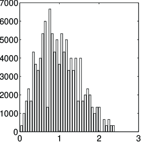
Figure 1: Distribution of spacings of a decomposable sandwich system.

A matrix connecting a decomposable vector ${\bf E}$, whose elements are not increasing, is obtained permuting the rows of (5), but, as we shall see, only the pemutations of a particular class are allowed for rows.

If, without loss of generality, we arrange the levels of $H^{q}_{1}$ and $H^{q}_{2}$ in increasing order, the eigenvalues of the total system must obey the following inequalities:

$$E_{i\,j+1}\geq E_{ij},\hskip 36.135ptE_{i+1\,j}\geq E_{ij};$$ (7)

the double indices have the same meaning as in eq. (1).

Let us take a decomposable system of levels, not necessarily sandwich, and arrange the eigenvalues in increasing order,

$$E_{i}>E_{j}\hskip 21.68121pt\mbox{if}\hskip 21.68121pti>j;$$ (8)

such a vector belongs to the range $K$ of $\cal M$, or to the kernel of the matrix (4), only if the system is sandwich: in all other cases an appropriate permutation exists such that the vector $E_{a(i)}\in K$. Inequality (8) implies that the elements of the new vector must preserve the original order, i.e.

$$E_{a(i)}>E_{a(j)}\hskip 21.68121pt\mbox{if}\hskip 21.68121pti>j.$$ (9)

A level of the total system can be denoted in two ways: with a double index — $E_{ij}$ — which shows that it is the sum of the $i-th$ level of the first system and the $j-th$ level of the second one, or with the usual single index that locates the element in vector ${\bf E}$. Therefore it is natural to single out the following association:

$$\begin{array}[]{ccc}(1,1)&\rightarrow&1\\ (1,2)&\rightarrow&2\\ \vdots&\vdots&\vdots\\ (1,n)&\rightarrow&n\\ \hline\cr(2,1)&\rightarrow&n+1\\ (2,2)&\rightarrow&n+2\\ \vdots&\vdots&\vdots\\ (2,n)&\rightarrow&2n\\ \hline\cr\vdots&\vdots&\vdots\\ \hline\cr(n,1)&\rightarrow&n(n-1)+1\\ (n,2)&\rightarrow&n(n-1)+2\\ \vdots&\vdots&\vdots\\ (n,n)&\rightarrow&n^{2}\end{array}.$$ (10)

This map will work for sandwich systems only; for a generic decomposable system we have to replace the second column with an appropriate permutation. The homogeneous system (6) now becomes

$$CT_{p}{\bf\Delta}=0,$$ (11)

where $T_{p}$ is obtained from matrix (5) by means of a suitable permutation of rows. In general with an arbitrary permutation the system (11) may not admit physical solutions, i.e. the spacings could be negative, or, equivalently, the system $C{\bf E}=0$ doesn’t have solutions verifying inequalities (7). The problem of locating the allowed permutations is equivalent to finding a particular class of maps $\cal A^{(p)}:\cal N^{2}\longmapsto\cal N$.

It is useful to denote the range of $\cal A^{(p)}$ by means of a $n$ by $n$ matrix $A^{(p)}$. From (9) and (10) it follows that a permutation is allowed if and only if

$$A_{i\,j+1}^{(p)}>A_{ij}^{(p)}\hskip 21.68121pt\mbox{ and }\hskip 21.68121ptA_{i+1\,j}^{(p)}>A_{ij}^{(p)};$$

this subclass of allowed permutations in $S_{n^{2}}$ is made up by all and only those maps which can be allocated in a matrix in such a way that the elements of the rows are strictly increasing from left to right and the elements of the columns are strictly increasing from top to bottom. It is well known that the number of permutations having this property is the dimension of the irreducible representation characterized by the corresponding square Young tableau.

It follows from the above considerations that the decomposability of a nonnegative vector ${\bf\Delta}$ is expressed in the most general way by the homogeneous systems (11), in which matrix $T_{p}$ is obtained from $T$ by means of a generic permutation of the columns and an allowed one of the rows.

It is important to point out, for what will follow, that the allowed permutations leave always the first and the last element fixed, so the elements of the first row of $T_{p}$ are all zero.

A detailed study of the kernels of all matrices $CT_{p}$ is necessary in order to classify all possible histograms of decomposable systems.

4 The chain of inequalities

The solution of the system (11), to make sense, must be made up of nonnegative elements. It follows that in our analysis we have to consider only the intersection of the kernel $K_{p}$ of the matrix $D_{p}=CT_{p}$ with the positive hyperoctant of $\cal R^{n^{2}-1}$. An arbitrary basis of a subspace is not, in general, formed by vectors whose elements are all nonnegative; moreover it is difficult to know a priori if a nonnegative vector exists in such a subspace, and, if it does, it is much more difficult to find it. Nevertheless it is easy to prove that if a vector of $K_{p}$ belongs to the positive hyperoctant (origin and coordinate hyperplanes excluded) then a whole basis made up of nonnegative vectors exists.

Let us find a basis of $K_{p}$. Let $\tilde{T}$ be a triangular matrix obtained removing the first row from matrix (5), and let $\tilde{T}_{p}^{-1}$ be the matrix obtained permuting the rows and the columns of $\tilde{T}^{-1}$ by means of the permutations applied to the columns and to the rows of (5), respectively, to obtain $T_{p}$. The allowed permutations contain $n^{2}$ elements, while the square matrices $\tilde{T}_{p}^{-1}$ have dimension $n^{2}-1$. This however is not a problem because the first row has been removed from the matrix $T$, and the allowed permutations do not change the first element; therefore to obtain the right permutation to apply to the columns of $\tilde{T}^{-1}$ it is enough to remove the first element of the corresponding allowed permutation and to subtract one from the other elements. So the matrix $\tilde{T}_{p}$ coincides with $T_{p}$ where the first row has been removed.

We have already noted that the kernel of (4) coincides with the range of (2). A basis of this subspace is made up of $2n-1$ arbitrary columns of the matrix $M$. Let $\tilde{M}$ be the matrix obtained from $M$ removing the first row: the matrix

$$T_{p}\tilde{T}_{p}^{-1}\tilde{M}$$ (12)

concides with $M$, except for the first row which now has every element equal to zero. Let $N$ be the submatrix of $\tilde{M}$ obtained removing the first and the $(n+1)-th$ column; the matrix

$$W=\tilde{T}_{p}^{-1}N$$ (13)

is made up of columns which, by construction, are vectors belonging to $K_{p}$; since $\tilde{T}_{p}^{-1}$ is obviously invertible, such vectors are linearly independent. We have excluded the first and the $(n+1)-th$ column of the matrix $\tilde{M}$, because their images through $T_{p}\tilde{T}_{p}^{-1}$ are the only columns of (12) which differ from the corresponding columns of $M$, and therefore do not belong to the kernel of (4). It is an easy exercise to prove that the vectors of $K_{p}$ so obtained are a maximal set of linearly independent vectors, i.e. that they are a basis.

The kernels of matrices $D_{p}$ are subspaces changing for different choices of the permutations applied to the rows and to the columns of (5): what we are interested in is a non-empty intersection of $K_{p}$ with the positive hyperoctant, it should be clear by now, that a permutation of the rows of (5) can shift this intersection outside the positive hyperoctant, whereas a permutation of the columns can only shift it inside.

Now we will find the conditions which must be satisfied by the coefficients of an arbitrary linear combination of the columns of (13) so that such a vector will be nonnegative; obviously we will restrict our analysis to matrixes $T_{p}$ whose rows are changed by allowed permutations.

The matrix $\tilde{T}^{-1}$ has the following structure:

$$\pmatrix{1&0&\cdots&0&0\cr-1&1&\cdots&0&0\cr 0&-1&\ddots&\vdots&\vdots\cr\vdots&\vdots&\ddots&1&0\cr 0&0&\cdots&-1&1\cr};$$ (14)

its analitical expression is the following:

$$\tilde{T}_{ij}^{-1}=\delta_{ij}-\delta_{i-1\,j};$$

the analitical expressions of the columns of the matrix $N$ are the following:

$$m_{i}^{r}=\sum_{k=1}^{n}\delta_{i\,n(k-1)+r}\hskip 21.68121ptr=1,2,\ldots,n-1,$$ (15)

$$m_{i}^{n-1+r}=\sum_{k=0}^{n-1}\delta_{i\,nr+k}\hskip 21.68121pti=1,2,\ldots,n^{2}-1.$$ (16)

Let $\tilde{T}_{p}^{-1}$ be obtained permuting the columns of $\tilde{T}^{-1}$ by means of an allowed permutation; multiplying on the right $\tilde{T}_{p}^{-1}$ by $N$ we have

$$\tilde{T}_{p}^{-1}N=\tilde{T}^{-1}N_{pi},$$ (17)

where $N_{pi}$ is obtained permuting the rows of $N$ with the inverse permutation of that applied to the columns of $\tilde{T}^{-1}$. Now formulae (15) and (16) become

$$m_{i}^{r}=\sum_{k=1}^{n}\delta_{a^{-1}(i)\;n(k-1)+r}\hskip 21.68121ptr=1,2,\ldots,n-1,$$ (18)

$$m_{i}^{n-1+r}=\sum_{k=0}^{n-1}\delta_{a^{-1}(i)\;nr+k}\hskip 21.68121pti=1,2,\ldots,n^{2}-1;$$ (19)

$a^{-1}(i)$ denotes the inverse permutation of the allowed one. Finally we obtain

$$W_{ir}=\delta_{a^{-1}(i)\;nq+r}-\delta_{a^{-1}(i-1)\;np+r}\hskip 21.68121pti=1,2,\ldots,n^{2}-1,$$ (20)

$$W_{i\,r+n-1}=\delta_{a^{-1}(i)\;nr+\tilde{p}}-\delta_{a^{-1}(i-1)\;nr+\tilde{q}}\hskip 21.68121ptr=1,2,\ldots,n-1;$$ (21)

$p,q,\tilde{p}\mbox{ and }\tilde{q}$ are indices running from $0$ to $n-1$. These expressions show that the second member of equation (20) is different from zero if the index $r$ coincides with the remainder of the division by $n$ of $a^{-1}(j)$ or $a^{-1}(j-1)$, while the second member of equation (21) is different from zero if the index $r$ is equal to the quotient of the same division. If we require that the individual elements of an arbitrary vector, linear combination of the columns of $W$, be strictly positive, we obtain the following chain of $n^{2}-1$ inequalities for the $2n-2$ coefficients of the linear combination:

$$C_{R_{a^{-1}(i)}}+\tilde{C}_{Q_{a^{-1}(i)}}>C_{R_{a^{-1}(i-1)}}+\tilde{C}_{Q_{a^{-1}(i-1)}};$$ (22)

$R_{a^{-1}(i)}$ denotes the remainder of the division by $n$ of $a^{-1}(j)$, while $Q_{a^{-1}(i)}$ its quotient. $C_{s}$ and $\tilde{C}_{s}$ are the coefficients of the columns of $W$, with the convention that they are zero when $s$ is equal to zero.

We can conclude that if the chain (22) admits solutions the kernel of the matrix $D_{p}$ intersects the positive hyperoctant and the solutions of inequalities (22) characterise completely the intersection.

The problem of classifying histograms compatible with such an intersection is still unsolved. In a histogram the choice of the width of the cells depends on the average number of elements per cell; in unfavourable cases, when the number of samples is small, few cells or few elements per cell yield a meaningless histogram, because a different choice of the cells changes completely its behaviour; when, on the contrary, the number of samples is large a variation of the width of the cells, in a reasonable interval, leaves its appearance unchanged. In what will follow we shall consider two histograms distinct if their cells have a different number of elements; clearly two different histograms in our convention may represent the same distribution, but, given the freedom in the choice of the cells and the algebraic nature of the problem, it is difficult to find a different approach. Nevertheless if one could carry out this classification one would succeed in identifying all the distributions compatible with decomposable systems.

In our analysis we will choose the unit of the spacings so that the cells have unitary width; moreover a histogram will be denoted by means of a set of $n^{2}-1$ integer $\{n_{k}\}$ such that

$$\sum_{k}n_{k}=n^{2}-1,$$ (23)

and such that the number of elements per cell $n_{k}$ is the number of spacings between $k-1$ and $k$. The elements of a vector ${\bf\Delta}$, not necessarily decomposable, denote a partition of $n^{2}-1$; they are also the coordinates of a point in the positive hyperoctant of $\cal R^{n^{2}-1}$ which is located in an hypercube whose edges have unitary length and whose vertices have integer and nonnegative coordinates. If we permute the elements of ${\bf\Delta}$, keeping fixed the coordinate system, the new vector will be, in general, in another hypercube, similar to the previous one and still consistent with the given histogram. It is easy to prove that the total number of hypercubes compatible with a given histogram is

$$\frac{(n^{2}-1)!}{n_{1}!n_{2}!\ldots n_{k}!}.$$ (24)

The cube in the positive hyperoctant defined by the relation

$$0\leq x_{i}\leq n^{2}-1\hskip 21.68121pti=1,2,\ldots,n^{2}-1$$ (25)

contains all the hypercubes compatible with histograms physically meaningful. Given a basis of $K_{p}$ and the solutions of inequalities (22), one may ask which unitary cubes contained in the cube (25) intersect $K_{p}$, i.e. which histograms are compatible with such a permutation. Clearly it is enough to consider kernels of matrices $D_{p}$ obtained permuting the rows of the matrix (5) but not its columns: permuting the element of a vector ${\bf\Delta}$ is tantamount as permuting the columns of (5); therefore if a kernel $K_{p}$ of $D_{p}=CT_{p}$, where $T_{p}$ is obtained permuting only the rows of $T$, intersects one of the cubes (24), so does any $K_{p}$ in which the columns of $T_{p}$ have been permuted with an arbitrary permutation.

Solving inequalities (22) is a formidable task, but even if we could do it— in some simple cases we have been able to solve the chain (22) by means of a computer (see fig. 2) —, we would still be faced with the problem of analysing the ensemble of histograms so generated.

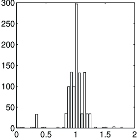
Figure 2: Distribution of spacings of a decomposable non sandwich system.

5 Conclusions

The example of the sandwich systems and the general study performed above suggest that the weight of decomposable systems whose spacing distributions are different from Poisson law is not negligible. The chain of inequalities (22) can be a starting point to give an answer. However our results are sufficient evidence that one cannot consider the distribution of spacings of the levels of a quantum system as the ”signature ” of the so called quantum chaos. It is worth to note that the we have not considered the semiclassical limit. Even if sometimes the behaviour for $\hbar\rightarrow 0$ can give hints on the properties of a system, it can also hide its very quantum nature.

References

- [1] Berry M.V and Tabor M., Proc. R. Soc. Lond. A., 356, 375–394, (1977).
- [2] Berry M.V., Ann. Phys., (N.Y.), 131, 163 (1981).
- [3] Bohigas O., Giannoni, M.J. and Schmit C., Phys. Rew. Lett, 52, 1 (1984).
- [4] Brody T.A., Flores J., French J.B., Mello P.A., Pandey A. and Wong S.S.M., Rev. Mod. Phys., 53, n. 3, 385–479, (1981).
- [5] Casati G., Chiricov B.V. and Guarnieri I., Phys. Rev. Lett., 54, 1350, (1985).
- [6] Casati G., Izrailev F. and Molinari L., J. Phys. A: Math and Gen., 24, 4755, (1991).
- [7] Colin de Verdiere Y.“Ergodcité et fonctions propres du Laplacien”, Sem. Bony-Sjöstrad-Meyer, 1984–1985, exposé no. XIII. Commun. Math. Phys., 102, 497–502, (1985)
- [8] Gutzwiller M.C.: “Chaos in Classical and Quantum Mechanics”, Springer Verlag, pgs. 432, (1990).
- [9] Metha M.L.: “Random Matrices and the Statistical Theory of Energy Levels”, Academic Pres, pgs. 259, (1967).
- [10] Paz J.P., Zurek W.H., “Quantum Chaos: A dechoerent definition”, preprint (1995)
- [11] Prosperi G. and Scotti A., J. Mat. Phys., 1, n. 3, 218–221, (1969).
- [12] Scotti A.: “A consistency criterion for ergodicity in Quantum Mechanics”, Symposium “Generalized Simmetries in Physics” Clausthal, Germany, 27–29 July, 1993.
- [13] Schnirelman A. I.: “Ergodic Properties of Eigenfunctions”, Ups. Math. Nauk., 29, 181–182, (1974).
- [14] Srednicki M. “Quantum Chaos and Statistical Mechanics”, Conference on Fundamental Problems in Quantum Theory, Baltimore, USA, June 18–22, 1994.
- [15] von Neuman J., Zschr. f. Physik, 57, 30–70, (1929).
- [16] Zelditch S.: “Quantum Ergodicity on the Sphere”, Comm. Math. Phys., Springer Verlag, (1992).