Spatiotemporal Dynamics of Mesoscopic Chaotic Systems

Abstract

An investigation of the mesoscopic dynamics of chemical systems whose mass action equation gives rise to a deterministic chaotic attractor is carried out. A reactive lattice-gas model for the three-variable autocatalator is used to provide a mesoscopic description of the dynamics. The global and local dynamics is studied as a function of system size and diffusion coefficient. When the diffusion length is comparable to the system size phase coherence is maintained but the amplitudes of the oscillations are uncorrelated due to interaction between fluctuations and the instability of the chaotic dynamics. If the diffusion length is small compared to the system size then phase turbulence serves to destroy the noisy global attractor.

I Introduction

The dynamics one observes on macroscopic scales has its origin in the molecular collision events that occur on the microscopic level. Under far-from-equilibrium conditions even the macroscopic dynamics can take complex forms and show chaotic or turbulent behavior. Macroscopic chaotic or ordered structures arise because the correlations extend to macroscopic scales. A complete understanding or description of the dynamics entails an examination of the system on the microscopic, or at least mesoscopic, length scales where internal fluctuations enter naturally in the dynamical description.

When the macroscopic deterministic dynamics is chaotic it is perhaps even more intriguing to consider how such structured chaotic motion for the macroscopic fields arises from the apparently random collision processes at smaller scales. We are then led to consider the interactions of fluctuations on small scales with the intrinsic instability of the chaotic dynamics on the macroscopic scales.

In this article we use a reactive lattice-gas automaton to provide a mesoscopic description of the reaction dynamics. We investigate a specific mass action chemical scheme, the three-variable autocatalator, which shows a period-doubling cascade to a chaotic attractor. The reaction scheme and its bifurcation structure are described in Sec. II. The lattice-gas model naturally incorporates local particle number fluctuations as a result of random local reactive events and particle motion. Section III provides details of the construction of the automaton dynamics and demonstrates that its mean field limit is the mass action rate law. The spatiotemporal dynamics in the chaotic regime is the subject of Sec. IV. The roles of internal fluctuations, diffusion and system size in determining the global and local dynamics are explored in this section. Section V presents a discussion of the automaton space and time scales and their relation to those in physical systems, while Sec. VI contains the conclusions of the study.

The automaton dynamics considered here not only provides a more fundamental description of far-from-equilibrium, chaotic, chemical systems but also constitutes a scheme for the study of such systems in the mesoscale domain where standard reaction-diffusion equation models may be inappropriate.

II Three-Variable Autocatalator Dynamics

In order to investigate the mesoscopic dynamics of systems exhibiting deterministic chaos it is necessary to consider reaction mechanisms with at least three species, apart from pool chemicals whose concentrations are maintained at fixed values by external feeds and constrain the system to lie far from equilibrium. It is also important that chemical concentrations remain positive and follow mass-action kinetics. In this article we consider the three-variable autocatalator[2] which has a rich phase space structure including periodic and chaotic attractors and allows us to investigate certain aspects of the dynamics without unnecessary complications arising from bistability in the relevant parameter range.

The three-variable autocatalator reaction mechanism is as follows[2]:

$$\begin{array}[]{rcl}A&\stackrel{{\scriptstyle k_{0}}}{{\longrightarrow}}&U\\ A+W&\stackrel{{\scriptstyle k_{1}}}{{\longrightarrow}}&U+W\\ U+2V&\stackrel{{\scriptstyle k_{2}}}{{\longrightarrow}}&3V\\ U&\stackrel{{\scriptstyle k_{3}}}{{\longrightarrow}}&V\\ V&\stackrel{{\scriptstyle k_{4}}}{{\longrightarrow}}&W\\ W&\stackrel{{\scriptstyle k_{5}}}{{\longrightarrow}}&B\;.\end{array}$$ (1)

The chemical dynamics is described by the variations in the $U$, $V$ and $W$ concentrations, while concentrations of $A$ and $B$ are taken to be fixed by feeds of these species; consequently thier concentrations can be regarded as bifurcation parameters. The mass action rate law corresponding to this mechanism is

$${d{\rho}_{u}\over dt} = \kappa_{0}+\kappa_{1}\rho_{w}-\kappa_{2}\rho_{u}\rho_{v}^{2}-\kappa_{3}\rho_{u}\,,$$ (2)

$${d{\rho}_{v}\over dt} = \kappa_{2}\rho_{u}\rho_{v}^{2}+\kappa_{3}\rho_{u}-\kappa_{4}\rho_{v}\,,$$ (3)

$${d{\rho}_{w}\over dt} = \kappa_{4}\rho_{v}-\kappa_{5}\rho_{w}\,.$$ (4)

Here $\rho_{\tau}(t)$ is the concentration of species $\tau=u,v,w$. The $\kappa_{i}$, $i=1,\cdots,5$, are effective rate constants that contain the concentrations of pool species. The system (3) has a steady state $(\rho_{u},\rho_{v},\rho_{w})=(u_{\rm s},v_{\rm s},w_{\rm s})$ where $u_{\rm s}=\kappa_{4}v_{\rm s}/(\kappa_{2}v^{2}_{\rm s}+\kappa_{3})$, $v_{\rm s}=\kappa_{0}\kappa_{5}/\kappa_{4}(\kappa_{5}-\kappa_{1})$ and $w_{\rm s}=\kappa_{4}v_{\rm s}/\kappa_{5}$. This steady state may be destabilized by a Hopf bifurcation at which a small-amplitude, oscillatory state emerges. In this study we choose $\kappa_{2}$ as the bifurcation parameter while the values of the other parameters are fixed at $\kappa_{0}=1.666667$, $\kappa_{1}=0.153$, $\kappa_{3}=0.02$, $\kappa_{4}=4.0$ and $\kappa_{5}=1.0$. With this choice of system parameters the Hopf bifurcation point occurs at $\kappa_{2}=\kappa_{2}^{\rm H}=15.68$. The steady state is stable for $\kappa_{2}>\kappa_{2}^{\rm H}$. When $\kappa_{2}$ is decreased a period doubling cascade leading to chaos is observed (cf. Fig. 1).

III Reactive Lattice-Gas Model

The mesoscale description of the autocatalator is based on a reactive lattice-gas model of the dynamics. The method of construction of such models along with specific applications have been described earlier[5, 6] and, consequently, only sketch of those features of the model that pertain to the present application will be given.

Imagine that each chemical species $X_{\tau}$ ($U=X_{1}$, $V=X_{2}$, $W=X_{3}$) resides on its own lattice ${\cal L}_{\tau}$. Each node of the species lattice ${\cal L}_{\tau}$ contains channels corresponding to unit velocities directed along the links of the lattice from a node to its nearest neighbors. The nodes of the species lattices have identical node labels ${\bf r}$ so that several different species may reside at the same spatial point in the system. There is no exclusion principle in the automaton model used in this study; $i.e.$, each velocity direction of a node on ${\cal L}_{\tau}$ may be occupied by any number of molecules $\alpha_{\tau}\geq 0$.

Particle diffusion occurs through successive applications of deterministic propagation of particles in directions determined by their velocities to neighboring lattice nodes, and velocity randomization where velocities are shuffled and particles are assigned new velocities at random. We denote the combination of propagation and velocity reandomization on ${\cal L}_{\tau}$ by $\hat{{\cal D}}_{\tau}$, the diffusion operator.

Consider a lattice ${\cal L}$ with ${\cal N}$ nodes labeled $({\bf r}_{1},{\bf r}_{2},\cdots,{\bf r}_{{\cal N}})$ and suppose many applications of the propagation and velocity randomization steps $\hat{{\cal D}}$ have been carried out. When there is no restriction on the number of particles at a node on a lattice, the equilibrium distribution of $n$ particles on ${\cal N}$ nodes is an occupancy problem. The probability of obtaining occupancy numbers $\alpha({\bf r}_{1}),\alpha({\bf r}_{2}),\cdots,\alpha({\bf r}_{\cal N})$ ($\alpha({\bf r}_{1})+\alpha({\bf r}_{2})+\cdots+\alpha({\bf r}_{\cal N})=n$) on ${\cal N}$ nodes is given by [8, 9]

$$P(\alpha({\bf r}_{1}),\alpha({\bf r}_{2}),\cdots,\alpha({\bf r}_{\cal N}))=\frac{n!}{\alpha({\bf r}_{1})!\alpha({\bf r}_{2})!\cdots\alpha({\bf r}_{\cal N})!}{\cal N}^{-n}\,.$$ (5)

The multimomial distribution (5) can be generated by the multinomial theorem

$$\left(p_{1}+p_{2}+\cdots+p_{\cal N}\right)^{n}=\sum_{\alpha({\bf r}_{1}),\alpha({\bf r}_{2}),\cdots,\alpha({\bf r}_{\cal N})}P(\alpha({\bf r}_{1}),\alpha({\bf r}_{2}),\cdots,\alpha({\bf r}_{\cal N}))\,,$$ (6)

with $p_{1}=p_{2}=\cdots=p_{\cal N}=1/{\cal N}$. To obtain the particle number distribution on a single node we sum over all the probabilities for the remaining ${\cal N}-1$ occupancy numbers:

$$P(\alpha({\bf r}_{1}))=\sum_{\alpha({\bf r}_{2}),\cdots,\alpha({\bf r}_{\cal N})}P(\alpha({\bf r}_{1}),\alpha({\bf r}_{2}),\cdots,\alpha({\bf r}_{\cal N}))\,.$$ (7)

The constraint on occupancy numbers $\alpha({\bf r}_{2}),\cdots,\alpha({\bf r}_{\cal N})$ in the sum is $\alpha({\bf r}_{2})+\cdots+\alpha({\bf r}_{\cal N})=n-\alpha({\bf r}_{1})$ with $0\leq\alpha({\bf r}_{1})\leq\alpha({\bf r}_{\cal N})$. Therefore we obtain

$$P(\alpha({\bf r}_{1}))=\frac{n!}{(n-\alpha({\bf r}_{1}))!\alpha({\bf r}_{1})!}\left(\frac{1}{\cal N}\right)^{\alpha({\bf r}_{1})}\left(1-\frac{1}{\cal N}\right)^{n-\alpha({\bf r}_{1})}\,,$$ (8)

where we have used the fact that

$$\sum_{\alpha({\bf r}_{2}),\cdots,\alpha({\bf r}_{\cal N})}\frac{(n-\alpha({\bf r}_{1}))!}{\alpha({\bf r}_{2})!\cdots\alpha({\bf r}_{\cal N})!}{\cal N}^{-(n-\alpha({\bf r}_{1}))}=[({\cal N}-1)/{\cal N}]^{n-\alpha({\bf r}_{1})}.$$ (9)

Since diffusion is carried out independently on all species lattices ${\cal L}_{\tau}$, we may simply append the label $\tau$ to the node occupancy numbers and suppress the node label since all nodes are equivalent. Thus the particle number distribution at a node on ${\cal L}_{\tau}$ is binomial:

$$P_{\rm b}(\alpha_{\tau})=\frac{n_{\tau}!}{(n_{\tau}-\alpha_{\tau})!\,\alpha_{\tau}!}\left(\frac{1}{\cal N}\right)^{\alpha_{\tau}}\left(1-\frac{1}{\cal N}\right)^{n_{\tau}-\alpha_{\tau}}\,,$$ (10)

where $n_{\tau}$ is the total number of particles on ${\cal L}_{\tau}$. If we let ${\cal N}\rightarrow\infty$ and $n_{\tau}\rightarrow\infty$ in such a way that the ratio $\rho_{\tau}=n_{\tau}/{\cal N}$ remains finite, the binomial distribution $P_{\rm b}(\alpha_{\tau})$ tends to the Poisson distribution[8, 9]:

$$P_{\rm p}(\alpha_{\tau})=\frac{(\bar{\rho}_{\tau})^{\alpha_{\tau}}}{\alpha_{\tau}!}\exp(-\bar{\rho}_{\tau})\,.$$ (11)

The automaton reactive dynamics at a node is controlled by the reaction operator $\hat{{\cal C}}$ whose action is encoded in the probability matrix $P(\mbox{\boldmath$\alpha$}|\mbox{\boldmath$\beta$})$. Each element of $P(\mbox{\boldmath$\alpha$}|\mbox{\boldmath$\beta$})$ gives the transition probability from a reactant particle configuration $\mbox{\boldmath$\alpha$}=(\alpha_{1},\alpha_{2},\cdots,\alpha_{s})$ to a product particle configuration $\mbox{\boldmath$\beta$}=(\beta_{1},\beta_{2},\cdots,\beta_{s})$, where $s$ is the number of species. If reaction is a rare event and diffusion is able to maintain spatial homogeneity over the lattice the local particle distribution will be homogeneous (binomial or Poisson). In this case the (discrete) mean field rate equation for the concentration changes is easily written in terms of the reaction probability matrix as

$${\rho}_{\tau}(t+1)-{\rho}_{\tau}(t)=\sum_{\mbox{\boldmath$\alpha$}}\sum_{\mbox{\boldmath$\beta$}}(\beta_{\tau}-\alpha_{\tau})P(\mbox{\boldmath$\alpha$}|\mbox{\boldmath$\beta$}){P}_{\rm h}\bigl{(}\mbox{\boldmath$\alpha$},\mbox{\boldmath$\rho$}(t)\bigr{)}\;,$$ (12)

where $P_{\rm h}\bigl{(}\mbox{\boldmath$\alpha$},\mbox{\boldmath$\rho$}(t)\bigr{)}=\Pi_{\tau}P_{\rm h}(\alpha_{\tau})|_{\bar{\rho}=\rho_{\tau}(t)}$ with $P_{\rm h}(\alpha_{\tau})=P_{\rm b}(\alpha_{\tau})$ or $P_{\rm p}(\alpha_{\tau})$. In the limit $n_{\tau}\rightarrow\infty$ ($\forall\tau$) and small reaction probabilities the mean field equation (12) should agree with the phenomenological mass action rate law (3). The reaction probability matrix $P(\mbox{\boldmath$\alpha$}|\mbox{\boldmath$\beta$})$ can be constructed so that this mean field limit is obtained. If we restrict particle number changes at a node to increases or decreases by one particle on each species lattice in accord with the mechanism of the reaction, one of the possible choices for the reaction probability matrix is

$$\begin{array}[]{rcl}P(\mbox{\boldmath$\alpha$}|\mbox{\boldmath$\beta$})&=&p_{1}(\mbox{\boldmath$\alpha$})\delta_{\beta_{u},\alpha_{u}+1}\delta_{\beta_{v},\alpha_{v}}\delta_{\beta_{w},\alpha_{w}}+p_{2}(\mbox{\boldmath$\alpha$})\delta_{\beta_{u},\alpha_{u}-1}\delta_{\beta_{v},\alpha_{v}+1}\delta_{\beta_{w},\alpha_{w}}\\ &+&p_{3}(\mbox{\boldmath$\alpha$})\delta_{\beta_{u},\alpha_{u}}\delta_{\beta_{v},\alpha_{v}-1}\delta_{\beta_{w},\alpha_{w}+1}+p_{4}(\mbox{\boldmath$\alpha$})\delta_{\beta_{u},\alpha_{u}}\delta_{\beta_{v},\alpha_{v}}\delta_{\beta_{w},\alpha_{w}-1}\,,\end{array}$$ (13)

where

$$p_{1}(\mbox{\boldmath$\alpha$}) = h(\kappa_{0}+\kappa_{1}\alpha_{w})\,,$$ (14)

$$p_{2}(\mbox{\boldmath$\alpha$}) = h[\kappa_{2}\alpha_{u}\alpha_{v}(\alpha_{v}-1)+\kappa_{3}\alpha_{u}]\,,$$ (15)

$$p_{3}(\mbox{\boldmath$\alpha$}) = h\kappa_{4}\alpha_{v}\,,$$ (16)

$$p_{4}(\mbox{\boldmath$\alpha$}) = h\kappa_{5}\alpha_{w}\,.$$ (17)

Here $h$ is a factor that determines the time scale in the automaton simulation. If (13) is inserted into (12) the mass action rate law (3) is recovered. Thus we may now investigate the full automaton dynamics and compare its behavior to the autocatalator mass action rate law and reaction-diffusion equation.

In summary, the automaton dynamics is specified by the compositions of the diffusion $\hat{{\cal D}}_{\tau}$ and reaction $\hat{{\cal C}}$ opertors:

$$\hat{T}=\prod_{\tau=1}^{s}\left(\hat{{\cal D}}_{\tau}\right)^{l_{\tau}}\circ\hat{C}^{l_{c}}\,.$$ (18)

In this equation $l_{\tau}$ and $l_{c}$ are non-negative integers, indicating that the operations are repeated $l_{\tau}$ and $l_{c}$ times, respectively. The reactive lattice gas model is a synchronously-updated, probabilistic cellular automaton.

The simulations reported in this paper were carried out on triangular lattices with ${\cal N}=N\times N$ nodes with periodic boundary conditions. On such triangular lattices the application of the diffusion operator $\hat{{\cal D}}$ yields a diffusion coefficient $D=1/4$ in units of lattice spacing squared per time step. For the composition rule in (18) the diffusion coefficient of species $\tau$ is given by $D_{\tau}=(l_{\tau}/l_{c})D$. In the simulations we have taken the diffusion coefficients to be equal: $D_{u}=D_{v}=D_{w}$. The time scale factor was taken to be $h=0.001$.

IV Spatiotemporal Dynamics in the Chaotic Regime

A complete understanding of the the dynamics of chaotic systems on mesoscopic scales involves the consideration of a number of different aspects. For systems which are sufficiently large and contain many particles but are well-mixed, either through diffusion or mechanical means, one expects that the chaotic attractor will resemble that of the mass action rate law, apart from modifications of the attractor structure on small phase-space scales.[11, 12, 13] If the system is large and molecular diffusion is the sole mechanism responsible for eliminating concentration gradients in the system then the full spatiotemporal dynamics must be considered. Even in such a circumstance there is interesting information in the global (spatially averaged) concentration fields and the attractors corresponding to these global variables; for example, for coupled map lattices composed of chaotic maps non-trivial, low-dimensional, global attractors have been observed.[14] The nature of such global attractors has also been studied in lattices of diffusively coupled Rössler oscillators where the local Rössler ODE dynamics is chaotic.[15] The description of all aspects of the noisy mesoscale dynamics involves a study of the spatial structure that underlies the temporal evolution. This section is devoted to an investigation of some of these issues for the autocatalator where we focus on the dynamics for $\kappa_{2}=11.52$, a parameter value lying in the chaotic regime.

A Noisy chaotic attractor: global dynamics

We observed above that if the system is small enough so that diffusion is able to maintain spatial homogeneity over the entire lattice but contains a sufficient number of particles that fluctuations in the mean concentrations are small, the automaton attractor constructed from the globally-averaged concentrations will closely resemble that determined from a solution of the mass-action ODE. Detailed studies of this type have been carried out for the Willamowski-Rössler model as a function of system size where the automaton rule has been modified to guarantee perfect mixing.[12] These calculations have confirmed that the gross structure of the chaotic attractor survives under the influence of internal noise, although noise can lead to destruction of fine-scale structure (e.g., band merging in banded attractors). There has been considerable discussion in the literature about the effects of internal noise in chaotic systems and detailed discussions can be found in Refs. [11, 12, 13, 16, 17].

As an example, for a lattice of size $32\times 32$ nodes we show that the noisy attractor (cf. Fig. 2(b)) constructed from the spatially-averaged concentrations,

$$\bar{\rho}_{\tau}(t)={N}^{-2}\sum_{{\bf r}\in{\cal L}_{\tau}}\rho_{\tau}({\bf r},t)\;,$$ (19)

resembles the deterministic attractor shown in panel (a) of Fig. 2, although there are noticeable effects due to fluctuations; as expected, the fluctuations tend to spread the dynamics in the unstable directions and obliterate some of the attractor structure. These effects diminsish as the system size increases provided spatial homogeneity can be maintained.[12]

Next, we consider the attractor structure determined from the spatially-averaged concentrations as a function of the system size for a fixed value of the diffusion coefficient, $D_{\tau}=1/4$. The results of a series of simulations on a set of $N\times N$ triangular lattices, with $N=64,\;128,\;256$ and $512$, are shown in Fig. 3. One observes that as $N$ increases the global attractor increasingly resembles a noisy periodic attractor whose width shrinks as the system size increases, at least on the time scale of the simulations. In the remainder of this section we examine the structure of the spatiotemporal dynamics that underlies this behavior.

B Spatiotemporal structure

We shall now examine in some detail the spatiotemporal dynamics on a $128\times 128$ lattice. The spatial structure that underlies global attractor discussed above is presented in Fig. 4. This figure shows the local concentration per node of species $U$ for different times (indicated by open squares) along a trajectory segment of the global attractor given in Fig. 5. Strong concentration gradients develop during the fast parts of the cycle while only small gradients exist during the slow parts of the cycle. Of course, this behavior is anticipated in view of the ability of diffusion to homogenize the concentration variations that arise from local reaction. The slow part of the cycle, $t_{s}$, comprises most of the average cycle time on the attractor, $t_{c}$. For the parameter value under consideration, $\kappa_{2}=11.52$, we have $t_{c}\sim 2.3$, while $t_{s}\sim 2.0$ and thus for the fast part of the cycle $t_{f}\sim 0.3$. Consequently, the diffusion lengths corresponding to these times are: $\ell_{D}^{s}\sim 32$ and $\ell_{D}^{f}\sim 12$ lattice sites, respectively. Since comparable concentration variations occur in the slow and fast parts of the cycle diffusion will clearly be able to more effectively homogenize the system in the slow part of the cycle than in the fast part of the cycle.

The spatiotemporal structure for the same parameters but on a $512\times 512$ lattice is shown in Fig. 6. Once again the strongest spatial inhomogeneities occur during the the fast part of the cycle but even in the slow parts, as is evident from the first three panels in the figure, one sees the small-amplitude inhomogeneities on the same length scale as in Fig. 4 more clearly since the system size is so much larger than the diffusion length.

The spatial structure may be examined in more detail by considering the coarse-grained dynamics of the system. For this purpose we divide the system into cells with linear dimension $L$ and define the coarse-grained concentration fields as,

$$\bar{\rho}_{\tau}(\bar{{\bf r}},t)=L^{-2}\sum_{{\bf r}\in{\cal L}_{\tau}(\bar{\bf r})}\rho_{\tau}({\bf r},t)\;,$$ (20)

where ${\cal L}_{\tau}(\bar{\bf r})$ is a domain of the lattice centered on $\bar{\bf r}$ containing $L\times L$ nodes. The time variations of $\bar{\rho}_{u}(\bar{{\bf r}},t)$ for four cells with $L=32$ are shown in Fig. 7. The chaotic oscillations in the individual cells remain in phase (at least over the time scale of the simulation) but their amplitudes vary erratically, especially during the transition from the slow part of the cycle to the fast part where fluctuations are strongly amplified. Such regions of the trajectory are expected to be most affected by noise arising from internal fluctuations.

Effects of this type were discussed earlier[19] in a consideration of the global dynamics of coupled map lattices with chaotic or periodic local elements. In the chaotic regime any internal fluctuation $\delta\rho_{\tau}({\bf r},0)$ will grow roughly as

$$\delta\bar{\rho}_{\tau}({\bf r},n_{c})=e^{\lambda t_{c}n_{c}}\delta\bar{\rho}_{\tau}({\bf r},0)\;,$$ (21)

where $n_{c}=t/t_{c}$ is the number of cycles on the chaotic attractor and $\lambda$ is the Lyapunov exponent. Here we have taken $\bar{\rho}_{\tau}(\bar{\bf r},t)$ to be the coarse-grained density. If the system is well-stirred the particle fluctuations at each node of the lattice should be Poisson distributed as discussed in the previous section. For finite diffusion, given the estimate of the diffusion length, one may expect Poisson-distributed fluctuations within the coarse-grained cells of size $L=32$. The Poisson fluctuations within such coarse-grained regions provide a source of perturbations of the dynamics of magnitude $\delta\bar{\rho}_{\tau}(\bar{\bf r},0)=(\bar{\rho}_{\tau})^{1/2}/L$ which are then amplified by the chaotic dynamics. One may then estimate the number of cycles on the attractor for the system to lose memory of its initial state as

$$n^{*}_{c}\sim{1\over\lambda t_{c}}\ln{\delta\bar{\rho}^{*}_{\tau}(\bar{\bf r})L\over(\bar{\rho}_{\tau})^{1/2}}\;,$$ (22)

where $\delta\bar{\rho}^{*}_{\tau}(\bar{\bf r})$ is a value of $\delta\bar{\rho}_{\tau}(\bar{\bf r},t)$ comparable to the “size” of the attractor in phase space. Using the cycle time on the attractor, $t_{c}\equiv 2.3$, and the fact that the Lyapunov exponemt is $\lambda=.229$ for $\kappa_{2}=11.52$ one finds that $n^{*}_{c}$ is of the order of a few cycles. Thus, given this time, one expects that regions separated by distances of order $\ell_{c}\sim(2Dt_{c}n^{*}_{c})^{1/2}$ will have the amplitudes of their oscillations uncorrelated. One finds $\ell_{c}\sim 33$ and thus the amplitudes in the $32\times 32$ coarse-grained cells should vary randomly as observed in the simulations. If one then spatially averages over the coarse-grained cells one should see noisy periodic dynamics since the random amplitudes will average to a nearly constant value. Note that phase coherence has not yet been destroyed and the above arguments apply to the structure transverse to the attractor.

It is interesting to compare the above dynamics with that in the periodic regime. The results for $\kappa_{2}=12.8$ are shown in Fig. 8 where panel (a) is the deterministic attractor and panel (b) is the attractor constructed from the global dynamics determined from a spatial average over the $128\times 128$ lattice. As expected, a noisy periodic attractor is obtained with strong amplification of the fluctuations in the fast part of the cycle. If one examines the coarse-grained dynamics that underlies the noisy periodic orbit (cf. Fig. 9) one sees local dynamics that is qualitatively similar to that for the chaotic dynamics described earlier: the internal fluctuations most strongly influence the the portion of the cycle where the dynamics changes from slow to fast, and phase coherence is maintained for this system size and value of the diffusion coefficient. In the periodic regime, from a linearized analysis of the dynamics, one expects the fluctuations about the deterministic motion to grow linearly with time.[16, 11] The fact that the dynamics observed in our simulations is similar in both the chaotic and periodic regimes likey reflects the small magnitude of the positive Lyapunov exponent for the autocatalator chaotic attractor. This implies that rather large spatial regions may remain correlated even in the chaotic regime. Similar persistence of correlations due to small positive values of the Lyapunov exponent were noted by Brunnet et al. [15] in studies of coupled Rössler ODEs.

In summary, the picture of the dynamics that is seen is consistent with the qualitative bifurcation diagram in Bohr et al.[19]; for the finite-amplitude noise arising from internal fluctuations in the dynamics one sees a noisy periodic orbit in both the chaotic and periodic regimes. For the relatively small lattice size, $128\times 128$, the system maintains phase coherence but noise interacts with the instability in the dynamics in directions along the unstable manifolds of the chaotic attractor to lead to erratic amplitude oscillations whose spatial average gives rise to a noisy periodic attractor.

C Destruction of phase coherence

As the system size increases, or alternatively the diffusion coefficient decreases, it will become impossible for the system to maintain phase coherence over the entire spatial domain.[20, 21] To investigate the passage to this regime we again consider $128\times 128$ lattices but vary the ratio $\ell_{\tau}/\ell_{r}$ to change the magnitude of the diffusion coefficient (and reactive time scale). In the automaton simulations we increase the value of $\ell_{r}$ keeping $\ell_{\tau}$ fixed so that the effective reaction rates are increased.

The global attractors for $D_{\tau}=D/6$ and $D/10$ are shown in Fig. 10. They shrink to a noisy fixed point attractor as synchronization of the phase in space is lost. This is easily confirmed from an examination of the coarse-grained dynamics in Fig. 11: now ones sees that both the amplitude and phase vary in the coarse-grained cells.

If the description of the dynamics were based on the reaction-diffusion equation it would be possible to account for changes in the overall reaction rates and diffusion coefficients by scaling space and time. If such scaling were valid, one could relate the automation simulations for fixed system parameters and varying system size to those for a fixed system size and varying parameters. This scaling is not valid as is evident from the results presented above. This signals a breakdown of the reaction-diffusion equation model for the fast reaction rates considered in this subsection. Here several reactions were carried out for each diffusion step giving rise to strong local fluctuations due to reactions which could not be smoothed by diffusion.

If one considers dynamics in the periodic regime ($\kappa_{2}=12.8$ described above) and decreases the diffusion coefficient or increases the system size, destruction of phase coherence is observed. Such destruction of phase coherence on large scales is well known in oscillatory media and gives rise to phase turbulence.[20] The present results for the chaotic regime show that even though the dynamics in smalll correlated regions is locally chaotic, phase coherence on the chaotic attractor is not maintained on long scales, a result that parallels that in oscillatory media. Thus, our stochastic reactive lattice-gas simulations of the autocatalator do not show a robust global periodic attractor that survives as the system size increases. In certain parameter regimes, such robust global attractors were seen in deterministic systems of coupled Rössler ODEs.[15]

V Space and Time Scales

A number of aspects of fluctuations and their effects on chaotic dynamics which were described above depend on the space and time scales involved in the automaton simulations. In order to use these results to interpret the behavior of physical systems one must establish a link between the scales in the automaton simulations and those that arise in real systems. Any connection of this type must take into account the characteristics of a specific system so we shall simply present a few order-of-magnitude estimates for representative cases to illustrate the points.

Consider a liquid-state (aqueous) reacting system where the reactants and products are small molecules. For a $0.01$M solution, a volume of solution with a linear dimension of $0.01\mu$ contains about three reactant molecules, a typical occupancy of an automaton node in our simulations. Thus, we may associate a linear dimension of $\ell_{a}=0.01\mu$ with the automaton lattice spacing. Taking the molecular diffusion coefficient to be $D\sim 10^{-5}\;{\rm cm}^{2}/{\rm s}$, the average time for a molecule to move by diffusion to a neighboring cell is $\ell_{a}^{2}/D=\tau_{a}\sim 0.1\;\mu{\rm s}$. This time can be associated with an automaton time step.

Next, we must consider the time scale of the reactive events in comparison with that for the non-reactive events, those that are largely responsible for the diffusion process, in order to see under what circumstances these scales may be applied. For this puropose we may use the average cycle time observed in the global dynamics. In the simulations presented in this paper the average cycle time was of order $t_{c}\sim 10^{3}$ time steps, and this corresponds to $t_{c}\sim 0.1\;{\rm ms}$, a rather fast chemical relaxation time for most typical oscillatory chemical reactions, but not unrealistic for reactions under certain conditions.

More usually the cycle time of many laboratory examples of oscillatory reactions lie in the range $1-100\;{\rm s}$. One may then work backward and associate a time of $10^{-3}\;{\rm s}$ with an automaton time step for a cycle time of $t_{c}=1\;{\rm s}$ from which it follows that the automaton cell dimension is roughly $10^{-4}\;{\rm cm}$ if the same value of the diffusion coefficient is used. In a cell volume of this size there are about $10^{7}$ reactant molecules so that the fluctuations in the automaton are about $10^{3}$ times larger than in a system of this type. Of course, these estimates serve to confirm that in usual circumtances, on the space and time scales of many macroscopic experiments, internal fluctuations play only a minor role. However, they are crucial in homogeneous nucleation processes and near bifurcation points they can play an essential role.

More importantly, the above calculations and estimates show that under not very extreme conditions, even less extreme if diffusion coefficients are smaller than our typical value, one may observe the consequences of the interactions between internal fluctuations and periodic or chaotic dynamics in the spatial domain.

VI Conclusion

The reactive lattice-gas automaton provides a description of the system at a mesoscopic level. On the smallest scales one has individual reactive events and random-walk dynamics. Of course, in general, at this level one must regard the particles as fictitious, representing some collection of real particles. However, one may consider physical circumstances where the particle numbers in the automaton correspond closely to those of a real system. In this case, the dynamics may be considered to be a model of real collision dynamics. At the coarse-grained level one observes a noisy version of the periodic or chaotic attractor. At this mesoscopic level one has interplay between the local periodic or chaotic dynamics, internal fluctuations and diffusion to give rise to the observed spatiotemporal structure.

In the chaotic regime internal fluctuations are amplified by the dynamcis and give rise to amplitude fluctuations in the coarse-grained concentration variables. Provided the diffusion length is large enough the system maintains phase coherence over all space and the phase space trajectory of the globallly-averaged concentrations lies on a noisy periodic attractor. In the periodic regime fluctuations from the deterministic limit cycle exhibit linear growth and a noisy limit cycle is also observed in this periodic regime. This behavior is consistent with earlier considerations of the noisy dynamcis of coupled map lattices.[19] If the diffusion length is sufficiently small then the chaotic system will no longer be able to maintain phase coherence and phase turbulence will ensue, similar to that seen in oscillatory media.

The reactive lattice-gas automaton is a synchronously-updated, probabilistic cellular automaton and thus shares some of the features that were seen to be essential in the observation of non-trivial global attractors.[14, 15] However, the well-stirred dynamics for large systems was seen to closely approximate that of the continuous-time mass action ODE. One may show in this limit that the mean field automaton equations are simply an Euler discretization of the mass action rate law. The time step in this discretization is controlled by the scale factor $h$ introduced in (13) and its small size insured that the automaton dynamics in this limit yielded results comparable to the solution of the underlying ODE. The reative lattice-gas model is intrinsically statistical in nature and encorporates the effects of internal fluctuations. Thus, there are a number of subtle issues involving the passage between disctete-time and continuous-time dynamics, and their implications for systems with broken time translation symmetry, that merit further investigation in the context of these models.

Acknowledgements: This work was supported in part by a grant from the Natural Sciences and Engineering Research Council of Canada and a by a Killam Research Fellowship (R.K.).

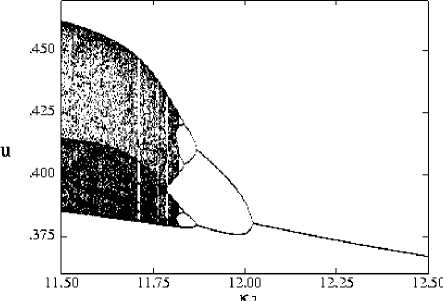
FIG. 1.: Bifurcation diagram constructed from the solution of the mass-action equations (2). Here $u$ and $w$, respectively, are $U$ and $W$ concentrations on a Poincaré section $P$, defined as $\{P:\,\rho_{v}=v_{\rm s},\,\forall\rho_{u},\rho_{w}\geq 0\}$. The bifurcation diagram shows the projection onto $u$ in the Poincaré section.

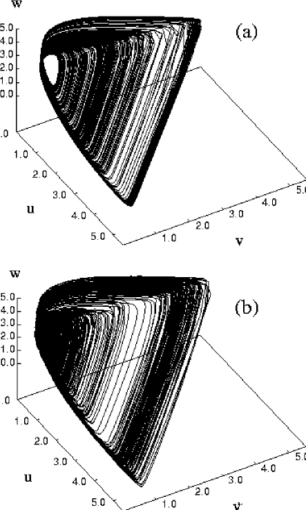
FIG. 2.: 3-D phase space plots of the chaotic attractor for $\kappa_{2}=11.52$: (a) mass action rate law (3) and (b) automaton simulation on a $32\times 32$ lattice.

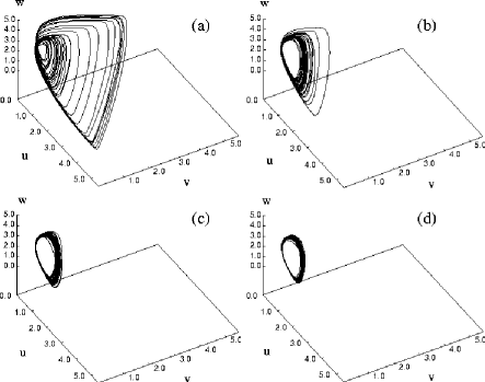
FIG. 3.: 3-D phase space plots of the global concentrations for $\kappa_{2}=11.52$ for various system sizes: (a) $64\times 64$ lattice, (b) $128\times 128$ lattice, (c) $256\times 256$ lattice and (d) $512\times 512$ lattice.

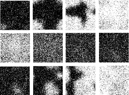
FIG. 4.: The twelve panels of this figure show the local concentrations of species $U$ for various times indicated in Fig. 5. Time increases from left to right and top to bottom and the total time spanned is about one and a half cycles on the attractor. The concentration is coded by gray shades with black high concentration and white low concentration of $U$.

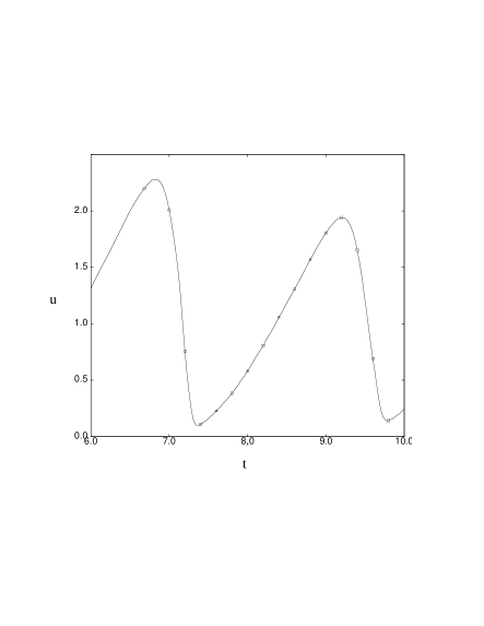
FIG. 5.: Plot of the global concentration of species $U$ in the time interval corresponding to the panels showing the spatial structure of the the $U$ concentration field. The points on the curve are taken at equally spaced time intervals. The panels in Fig. 4 correspond to the open squares while the open triangles denote intermediate times where the structure is not displayed.

FIG. 6.: The six panels of this figure show the local concentrations of species $U$ on a $512\times 512$ lattice for various times within one cycle on the global attractor. Time increases from left to right and top to bottom. The concentration is coded by gray shades with black high concentration and white low concentration of $U$.

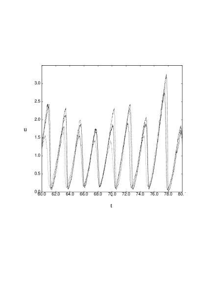
FIG. 7.: Plot of the coarse-grained concentration of species $U$, $\bar{\rho}_{u}(\bar{{\bf r}},t)$, in four cells as a function of time for $\kappa_{2}=11.52$.

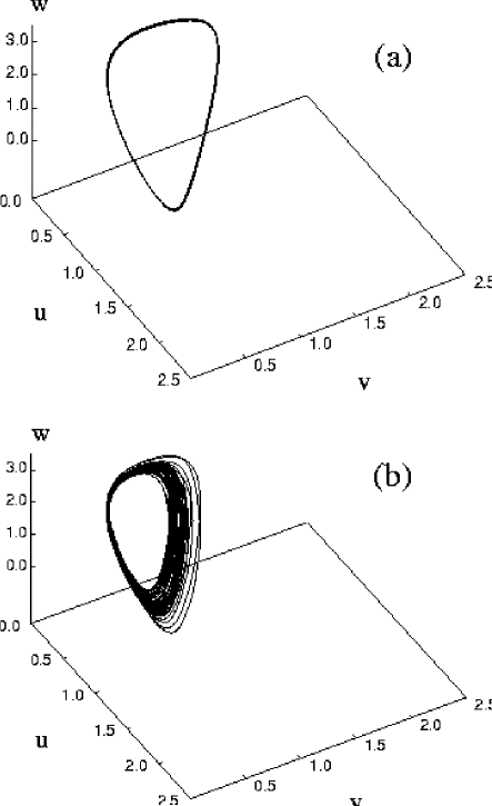
FIG. 8.: Global phase space dynamics for $\kappa_{2}=12.8$, a parameter value in the periodic regime, for (a) the deterministic mass action rate law (3) and (b) automaton dynamics on a $128\times 128$ lattice.

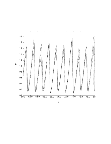
FIG. 9.: Plot of the coarse-grained concentration of species $U$, $\bar{\rho}_{u}(\bar{{\bf r}},t)$, in four cells as a function of time for $\kappa_{2}=12.8$.

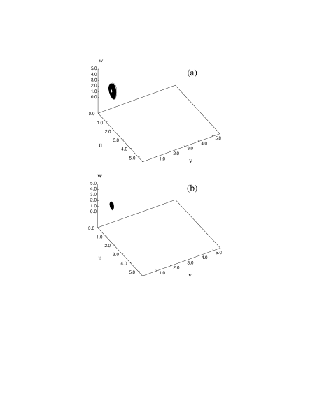
FIG. 10.: Phase space plots of the global atractors determined from automaton dynamics on $128\times 128$ lattices for two values of the diffusion coefficient: (a) $D_{\tau}=D/6$ and (b) $D_{\tau}=D/10$.

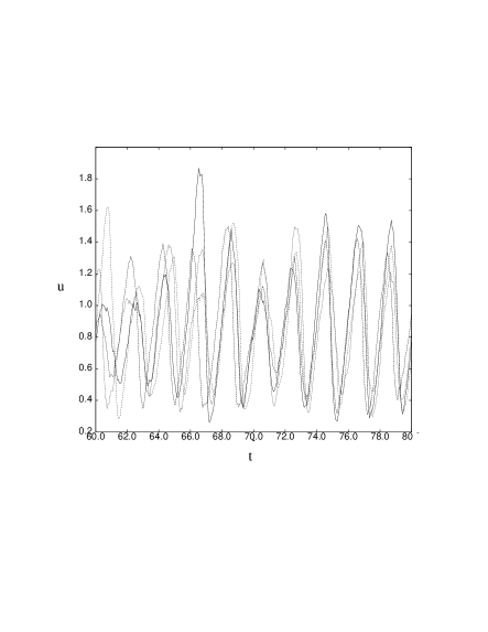
FIG. 11.: Plot of the coarse-grained concentration of species $U$, $\bar{\rho}_{u}(\bar{{\bf r}},t)$, in four cells as a function of time for $\kappa_{2}=11.52$ for $D_{\tau}=D/6$.

REFERENCES

- [1] K.-D. Willamowski and O.E. Rössler, Z. Naturforsch. Teil A 35, 317 (1980).
- [2] B. Peng, S.K. Scott and K. Showalter, J. Phys. Chem. 94, 5243 (1990).
- [3] P. Gray and S. K. Scott, Ber. Bunsen-Ges. Phys. Chem. 90, 985 (1986).
- [4] R. Kapral and X.-G. Wu, Annals N. Y. Acad. Sci. 706, 186 (1993) and J. Guemez and M. Matias, Phys. Rev. E 48, R2351 (1993).
- [5] J.-P. Boon, D. Dab, R. Kapral and A. Lawniczak, Physics Reports, (1996), to be published.
- [6] D. Dab, A. Lawniczak, J.-P. Boon and R. Kapral, Phys. Rev. Lett. 64, 2462 (1990); A. Lawniczak, D. Dab, R. Kapral and J.-P. Boon, Physica D 47, 132 (1991); R. Kapral, A. Lawniczak and P. Masiar, Phys. Rev. Lett. 66, 2539 (1991); J. Chem. Phys. 96, 2762 (1992); D. Dab, J.P. Boon and Y.-X. Li, Phys. Rev. Lett. 66, 2535 (1991).
- [7] B. Chopard, M. Droz, S. Cornell and L. Frachebourg, in Cellular Automata for Astrophysics, J. Perdang and A. Lejeune,eds. (World Scientific, Singapore, 1994); T. Karapiperis and B. Blankleider, Physica D 78, 30 (1994).
- [8] J.G. Kalbfleisch, Probability and Statistical Inference, Vol. 1 (Springer, New York, 1985).
- [9] W. Feller, An Introduction to Probability Theory and Its Applications, Vol. II (Wiley, New York, 1966).
- [10] G. Nicolis and I. Prigogine, Self-Organization in Non-Equilibrium Systems, (Wiley, New York, 1977); N. G. van Kampen, Stochastic Processes in Physics and Chemistry (North-Holland, Amsterdam, 1981).
- [11] X.-G. Wu, and R. Kapral, Phys. Rev. Lett. 70, 1940 (1993); J. Chem. Phys. 100, 5936 (1994).
- [12] X.-G. Wu and R. Kapral, Phys. Rev. E 50, 3560 (1994).
- [13] G. Nicolis and V. Balakrishnan, Phys. Rev. A 46, 3569 (1992); P. Peters and G. Nicolis, Physica A 188, 426 (1992); P. Geysermans and G. Nicolis, J. Chem. Phys. (1994); G. Nicolis, F. Baras, P. Geysermans and P. Peeters, in Chemical Waves and Patterns, eds. R. Kapral and K. Showalter, (Kluwer, Dordrecht, 1995); F. Baras and P. Geysermans, Nuovo Cimento, 17D, 709 (1995).
- [14] H. Chaté and P. Manneville, Europhys. Lett. 17, 291 (1992); Prog. Theor. Phys. 87, 1 (1992).
- [15] L. Brunnet, H. Chaté and P. Manneville, Physica D 78, 141 (1994).
- [16] R.F. Fox, Phys. Rev. A 41, 2960 (1990); 42, 1946 (1990); R.F. Fox and J. Keizer, Phys. Rev. Lett. 64, 249 (1990); Phys. Rev. A 43, 1709 (1991); J.E. Keizer and R.F. Fox, Phys. Rev. A 46, 3572 (1992); J. Keizer and J. Tilden, J. Phys. Chem. 93, 2811 (1989); R.F. Fox and T.C. Elston, to be published.
- [17] R. Kapral and X.-G. Wu, in Chemical Waves and Patterns, eds. R. Kapral and K. Showalter (Kluwer, Dordrecht, 1995).
- [18] R. Kapral, M. Schell and S. Fraser, J. Phys. Chem. 86, 2205 (1982); E. Celarier and R. Kapral, J. Chem. Phys. 86, 3366 (1987).
- [19] T. Bohr, G. Grinstein, Y. He and C. Jayaprakash, Phys. Rev. Lett. 58, 2155 (1987).
- [20] Y. Kuramoto, Chemical Oscillations, Waves and Turbulence, (Springer, Berlin, 1980).
- [21] C. Bennett, G. Grinstein, Y. He, C. Jayaprakash and D. Mukamel, Phys. Rev. A 41, 1932 (1990).