Tools for Nonlinear Analysis:
I. Unfolding of Dynamical Systems.

Abstract

Automated algorithms for derivation of amplitude equations in the vicinity of monotonic and Hopf bifurcation manifolds are presented. The implementation is based on Mathematica programming, and is illustrated by several examples.

1 Introduction

Amplitude equations describe behavior of evolutionary systems in the vicinity of threshold, or critical values of parameters that mark a point of qualitative change in behavior, like a transition from a quiescent state to convection, or from rigid mechanical equilibrium to vibration, or from a homogenious to patterned state of a material medium. Near the criticality, the behavior of systems of different physical origin is described by representative equations belonging to one of universal classes that are determined by the character of the transition.

There is a number of celebrated “universal” equations which have been extensively studied in physical literature. Some of them were first suggested as models, others were derived as rational approximations in a certain physical context, and then discovered again in apparently unrelated problems. The general structure of these equations can be often predicted by symmetry considerations. The algorithms of their derivation, known as center manifold methods in mathematical literature [Guckenheimer & Holmes, 1983; Hale & Koçak, 1991], or elimination of “slaved” variables in physical literature [Haken, 1987], are well established, at least in standard cases. However, actual computations required for establishing quantitative relations between the coefficients of amplitude equations and parameters of underlying physical systems are repetitive and time-consuming, and have been carried out in scientific literature on a case-to-case basis.

It is important to note that, except simplest cases when coefficients can be removed by rescaling, different qualitative features of the behavior are observed in different parameter ranges. When relations between coefficients of universal equations and measurable physical parameters are known, the domains determined by studying universal equations can be mapped upon the actual parameter space, and then further continued into a region where universal equations are no longer valid quantitatively but still faithfully describe qualitative features of behavior of a complex nonlinear system.

The aim of this communication is to describe the Mathematica-based automated algorithm for derivation of amplitude equations in either symbolic or numerical form. The algorithm makes use of Mathematica capabilities as a programming language [Wolfram, 1991] that allow to define special functions carrying out complicated tasks in response to simple and well-defined inputs. The paper is organized as follows. The general algorithm based on multiscale bifurcation expansion is outlined in Section 2. The three functions designed to implement the algorithm of bifurcation expansion – BifurcationCondition, BifurcationTheory, and Unfolding are described in Section 3. Several examples of usage of these functions for derivation of amplitude equations for dynamical systems are given in Section 4. Further generalization of the algorithm to distributed systems will be described in forthcoming communications.

2 General Algorithm

2.1 Multiscale Expansion

The general standard algorithm for derivation of amplitude equations is based on multiscale expansion of an underlying dynamical system in the vicinity of a bifurcation point. Consider a set of first-order ordinary differential equations in ${\sf R}^{n}$:

$$d{\bf u}/dt={\bf f}({\bf u},{\bf p}),$$ (1)

where ${\bf f}({\bf u};{\bf p})$ is a real-valued vector-function of an array of dynamic variables ${\bf u}$, that is also dependent on an array of parameters ${\bf p}$. We expand both variables and parameters in powers of a dummy small parameter $\epsilon$:

$${\bf u} = {\bf u}_{0}+\epsilon{\bf u}_{1}+\epsilon^{2}{\bf u}_{2}+\ldots,$$

$${\bf p} = {\bf p}_{0}+\epsilon{\bf p}_{1}+\epsilon^{2}{\bf p}_{2}+\ldots.$$ (2)

We shall also introduce a hierarchy of time scales $t_{k}$ rescaled by the factor $\epsilon^{k}$, thus replacing the function ${\bf u}(t)$ by the function of an array of rescaled time variables. Accordingly, the time derivative is expanded in a series of partial derivatives $\partial_{k}\equiv\partial/\partial t_{k}$:

$$\frac{d}{dt}=\partial_{0}+\epsilon\partial_{1}+\epsilon^{2}\partial_{2}+\ldots.$$ (3)

Let ${\bf u}={\bf u}_{0}({\bf p}_{0})$ be an equilibrium (a fixed point) of the dynamical system (1), i.e. a zero of the vector-function ${\bf f}({\bf u};{\bf p})$ at a point ${\bf p}={\bf p}_{0}$ in the parametric space. The function ${\bf f}({\bf u};{\bf p})$ can be expanded in the vicinity of ${\bf u}_{0},{\bf p}_{0}$ in Taylor series in both variables and parameters:

$${\bf f}({\bf u};{\bf p}) = {\bf f_{u}}({\bf u}-{\bf u}_{0})+\frac{1}{2}{\bf f_{uu}}({\bf u}-{\bf u}_{0})^{2}+\frac{1}{6}{\bf f_{uuu}}({\bf u}-{\bf u}_{0})^{3}+\ldots$$ (4)

$$+ {\bf f_{p}}({\bf p}-{\bf p}_{0})+{\bf f_{up}}({\bf u}-{\bf u}_{0})({\bf p}-{\bf p}_{0})+\frac{1}{2}{\bf f_{uup}}({\bf u}-{\bf u}_{0})^{2}({\bf p}-{\bf p}_{0})+\ldots.$$

The derivatives with respect to both variables and parameters ${\bf f_{u}}=\partial{\bf f}/\partial{\bf u},\;{\bf f_{uu}}=\partial^{2}{\bf f}/\partial{\bf u}^{2},\;{\bf f_{p}}=\partial{\bf f}/\partial{\bf p},\;{\bf f_{up}}=\partial^{2}{\bf f}/\partial{\bf u}\partial{\bf p}$, etc., are evaluated at ${\bf u}={\bf u}_{0},\;{\bf p}={\bf p}_{0}$.

Using Eqs. (2) – (4) in Eq. (1) yields in the first order

$$\partial_{0}{\bf u}_{1}={\bf f_{u}u}_{1}+{\bf f_{p}p}_{1}.$$ (5)

The homogeneous linear equation

$${\cal L}{\bf u}_{1}\equiv({\bf f_{u}}-\partial/\partial t_{0}){\bf u}_{1}=0$$ (6)

obtained by setting in Eq. (5) ${\bf p}_{1}=0$ governs stability of the stationary state ${\bf u}={\bf u}_{0}$ to infinitesimal perturbations. The state is stable if all eigenvalues of the Jacobi matrix ${\bf f_{u}}$ have negative real parts. This can be checked with the help of the standard Mathematica function Eigenvalues. Computation of all eigenvalues is, however, superfluous, since stability of a fixed point is determined by the location in the complex plane of a leading eigenvalue, i.e. that with the largest real part. Generically, the real part of the leading eigenvalue vanishes on a codimension one subspace of the parametric space called a bifurcation manifold. The two types of codimension one bifurcations that can be located by local (linear) analysis are a monotonic bifurcation where a real leading eigenvalue vanishes, and a Hopf bifurcation where a leading pair of complex conjugate eigenvalues is purely imaginary. Additional conditions may define bifurcation manifolds of higher codimension.

2.2 Monotonic Bifurcation

A monotonic bifurcation is also a bifurcation of equilibria of the dynamical system (1). Setting ${\bf u}_{1}$ = const, i.e. $\partial_{0}{\bf u}_{1}=0$, allows to find a shift of the stationary solution due to small variations of parameters

$${\bf u}_{1}=-{\bf f_{u}}^{-1}{\bf f_{p}p}_{1}.$$ (7)

The $n\times m$ array ${\bf f_{u}}^{-1}{\bf f_{p}}$ is recognized as a parametric sensitivity matrix; ($m$ denotes the dimension of the parametric space). Continuous dependence on parameters can be used to construct a branch of equilibria which terminates at a bifurcation point ${\bf p}_{0}$.

On a monotonic bifurcation manifold, the matrix ${\bf f_{u}}$ has no inverse. This means that one can neither construct a stationary solution at values of parameters close to this point, nor characterize the stability of the equilibrium in the linear approximation. The dynamics in the vicinity of the bifurcation manifold is governed by a nonlinear amplitude equation to be obtained in higher orders of the expansion.

Generically, the zero eigenvalue is non-degenerate. Let ${\bf U}$ be the corresponding eigenvector satisfying ${\bf f_{u}U}=0$. Then

$${\bf u}_{1}=a(t_{1},t_{2},\ldots){\bf U}$$ (8)

is the solution of Eq. (6) that remains stationary on the fast time scale $t_{0}$. The amplitude $a$ is so far indeterminate, and may depend on slower time scales.

The inhomogeneous equation Eq. (5) has solutions constant on the rapid time scale, provided its inhomogeneity does not project on the eigenvector U. This condition is

$$\kappa_{1}\equiv{\bf U}^{\dagger}{\bf f_{p}p}_{1}=0,$$ (9)

where ${\bf U}^{\dagger}$ is the eigenvector of the transposed matrix ${\bf f_{u}}^{\dagger}={\tt Transpose}[{\bf f_{u}}]$ satisfying ${\bf f_{u}}^{\dagger}{\bf U}^{\dagger}=0$; we assume that the eigenvector is normalized: ${\bf U}^{\dagger}{\bf U}=1$. Eq. (9) defines the tangent hyperplane to the bifurcation manifold at the point ${\bf p}_{2}={\bf p}_{0}$.

Before writing up the second-order equation, we require that the second-order deviation ${\bf u}_{2}$ remain constant on the rapid time scale (otherwise it may outgrow ${\bf u}_{1}$ at long times). The dependence on slower time scales must be expressed exclusively through the time dependence of the amplitude $a$. Using Eq. (8), we write the second-order equation as

$${\bf f_{u}u}_{2}=\partial_{1}a{\bf U}-{\bf f_{p}p}_{2}-a{\bf f_{up}Up}_{1}-\frac{1}{2}a^{2}{\bf f_{uu}UU}.$$ (10)

The solvability condition of this equation is

$$\partial_{1}a=\kappa_{2}+\lambda_{1}a-\mu_{0}a^{2}.$$ (11)

The parameters of Eq. (11) are

$$\kappa_{2}={\bf U}^{\dagger}{\bf f_{p}p}_{2},\;\;\lambda_{1}={\bf U}^{\dagger}{\bf f_{up}Up}_{1},\;\;\mu_{0}=-\frac{1}{2}{\bf U}^{\dagger}{\bf f_{uu}UU}.$$ (12)

The indices correspond to the scaling of respective parametric deviations from the bifurcation point. In a generic case, one can consider only parametric deviations transverse to the bifurcation manifold, and set ${\bf p}_{1}=0$ to satisfy Eq. (9); then $\lambda_{1}=0$. Thus, the generic equation for slow dynamics near the bifurcation manifold is

$$\partial_{1}a=\kappa_{2}-\mu_{0}a^{2}.$$ (13)

On the one side of the bifurcation manifold, where $\kappa_{2}$ has the same sign as $\mu_{0}$, there are two stationary states $a=\pm\sqrt{\kappa_{2}/\mu_{0}}$. When viewed as a solution of Eq. (13), one of them is stable, and the other, unstable. The stable solution corresponds to a stable equilibrium of the original system Eq. (1), provided the rest of eigenvalues of the matrix ${\bf f_{u}}$ have negative real parts. On the other side of the bifurcation manifold, where the signs $\kappa_{2}$ and $\mu_{0}$ are opposite, there are no stationary states. The trajectory of the dynamical system is deflected then to another attractor, far removed from ${\bf u}_{0}$. Thus, the system undergoes a first-order phase transition when the bifurcation manifold is crossed. If the value of some dynamic variable or other characteristic of the solution is drawn as a function of parameters, the bifuration locus can be seen as the projection of a fold of the solution manifold on the parametric plane; accordingly, the generic monotonic bifurcation is also called a fold bifurcation.

It may happen that the matrix ${\bf f_{p}}$ vanishes identically. This would be the case when ${\bf u}_{0}$ is a “trivial” solution that remains constant at all values of parameters. Then Eq. (9) is satisfied identically, and Eq. (11) reduces to

$$\partial_{1}a=\lambda_{1}a-\mu_{0}a^{2}.$$ (14)

This equation has two solutions, $a=0$ and $a=\lambda_{1}/\mu_{2}$, on both sides of the bifurcation manifold, but the two solutions interchange stability when this manifold is crossed.

2.3 Unfolding of Higher-Order Bifurcations

If $\mu_{0}=0$, the expansion should be continued to the next order. The coefficient $\mu_{0}$ may vanish identically due to the symmetry of the original problem to inversion of u. Otherwise, it may be equal to zero at certain values of the parameters of the problem. Generally, the two conditions, Det$[{\bf f_{u}}]=0$ and $\mu_{0}=0$ are satisfied simultaneously on a codimension two manifold in the parametric space that corresponds to a cusp singularity.

In order to continue the expansion, we restrict parametric deviations in such a way that the dependence on $t_{1}$ be suppressed. Deviations transverse to the bifurcation manifold have to be restricted by the condition $\kappa_{2}=0$, which is stronger than Eq. (9). First-order parametric deviations ${\bf p}_{1}$ parallel to the bifurcation manifold, which are still allowed by Eq. (9), should be now restricted by the condition $\lambda_{1}=0$. If the array p contains two parameters only, the conditions $\lambda_{1}=0$ and $\kappa_{1}=0$ imply, in a non-degenerate case, that first-order parametric deviations should vanish identically. When more parameters are available, parametric deviations satisfying both these conditions are superfluous, since they correspond just to gliding into a closer vicinity of another point on the cusp bifurcation manifold in a higher-dimensional parametric space. Further on, we shall set therefore ${\bf p}_{1}$ to zero identically.

The dynamics unfolding on a still slower time scale $t_{2}$ should be determined from the third-order equation

$${\bf f_{u}u}_{3}=\partial_{2}a{\bf U}-{\bf f_{p}p}_{3}-a{\bf f_{up}Up}_{2}-a{\bf f_{uu}Uu}_{2}-\frac{1}{6}a^{3}{\bf f_{uuu}UUU}.$$ (15)

The second-order function ${\bf u}_{2}$ has to be found by solving Eq. (10), now reduced to the form

$${\bf f_{u}u}_{2}={\bf f_{p}p}_{2}+\frac{1}{2}a^{2}{\bf f_{uu}UU}.$$ (16)

Only the solution of the inhomogeneous equation, which does not project on the eigenvector U, is relevant. It can be expressed as

$${\bf u}_{2}={\bf U}_{2}^{(2)}+a^{2}{\bf U}_{2}^{(0)}.$$ (17)

The solvability condition of Eq. (15) is obtained then in the form

$$\partial_{2}a=\kappa_{3}+\lambda_{2}a-\nu_{0}a^{3},$$ (18)

where

$$\kappa_{3} = {\bf U}^{\dagger}{\bf f_{p}p}_{3},$$

$$\lambda_{2} = {\bf U}^{\dagger}{\bf f_{up}Up}_{2}+{\bf U}^{\dagger}{\bf f_{uu}UU}_{2}^{(2)},$$

$$\nu_{0} = -\frac{1}{6}{\bf U}^{\dagger}{\bf f_{uuu}UUU}-{\bf U}^{\dagger}{\bf f_{uu}UU}_{2}^{(0)}.$$ (19)

Eq. (18) presents the parametric unfolding of dynamics in the vicinity of a cusp bifurcation. Three equilibria – two stable and one unstable – exist in the cusped region

$$\lambda_{2}>0,\;\;\;|\kappa_{3}|<\frac{2\lambda^{3/2}}{3^{3/2}\nu^{1/2}}.$$ (20)

Outside this region, there is a unique stable equilibrium. A second-order phase transition occurs when the parameters change in such a way that $\lambda_{2}$ crosses zero. Other transitions occuring in the vicinity of the cusp bifurcation are weakly first-order.

The condition $\nu_{0}=0$ defines a singular bifurcation manifold of codimension three. Again, it is possible to fix parametric deviations to suppress the dynamics on the scale $t_{2}$, and obtain in the next order a quatric equation that represents the unfolding of the butterfly singularity. The procedure can be continued further if a sufficient number of free parameters is available. The unfolding of a codimension $q$ singularity is presented by a polynomial of order $q+1$:

$$\partial_{q}a=\sum_{p=0}^{q-1}\sigma_{q-p+1}a^{p}-\sigma_{0}a^{q+1},$$ (21)

where the parameters $\sigma_{k}$ depend on parametric deviations proportional to $\epsilon^{k}$.

2.4 Hopf Bifurcation

At the Hopf bifurcation point, the parametric dependence of the stationary solution ${\bf u}={\bf u}_{0}({\bf p})$ remains smooth; linear corrections can be obtained from the stationary eq. (7), and higher corrections from higher orders of the regular expansion (4). In order to simplify derivations, we shall eliminate this trivial parametric dependence by transforming to a new variable $\hat{{\bf u}}={\bf u}-{\bf u}_{0}({\bf p})$. The resulting dynamic system, $d\hat{{\bf u}}/dt=\hat{{\bf f}}(\hat{{\bf u}},{\bf p})$ has the same form as (1) but contains a modified vector-function $\hat{{\bf f}}(\hat{{\bf u}},{\bf p})={\bf f}(\hat{{\bf u}}+{\bf u}_{0},{\bf p})$. Since, by definition, ${\bf u}_{0}$ satisfies ${\bf f}({\bf u}_{0},{\bf p})=0$, $\hat{{\bf u}}=0$ is a zero of $\hat{{\bf f}}({\bf u},{\bf p}).$ Now we can drop the hats over the symbols and revert to the original form (1) while keeping in mind that ${\bf u}=0$ is a stationary solution for all ${\bf p}$ and, consequently, all derivatives ${\bf f_{p},f_{pp}}$, etc., computed at ${\bf u}=0$ vanish.

At a Hopf bifurcation point the Jacobi matrix ${\bf f_{u}}$ has a pair of imaginary eigenvalues $\lambda=\pm i\omega_{0}$. The first order equation (6) has a nontrivial oscillatory solution

$${\bf u}_{1}=a(t_{1},t_{2},\ldots)\Phi(t_{0})+c.c.;\ \ \ \ \ \Phi(t_{0})=e^{i\omega_{0}t_{0}}{\bf U}$$ (22)

with an arbitrary complex amplitude $a(t_{1},t_{2},\ldots)$ dependent on slower time scales $t_{i},\;i>0$; ${\bf U}$ is the eigenvector of ${\bf f_{u}}$ with eigenvalue $i\omega_{0}$:

$${\bf f_{u}U}=i\omega_{0}{\bf U}.$$ (23)

The function $\Phi(t_{0})$ and its complex conjugate $\Phi^{\ast}(t_{0})$ are two eigenfunctions of the linear operator ${\cal L}$ with zero eigenvalue. The operator ${\cal L}$ is defined in the space of $2\pi/\omega_{0}$-periodic complex-valued vector-functions with the scalar product defined as

$$\langle{\bf u},{\bf v}\rangle=\frac{\omega_{0}}{2\pi}\int_{0}^{2\pi/\omega_{0}}{\bf u}^{\ast}(t)\cdot{\bf v}(t)dt.$$ (24)

The eigenfunctions of the adjoint operator ${\cal L}^{{\dagger}}={\bf f_{u}}^{{\dagger}}+\partial/\partial t_{0}$ are

$$\Phi^{{\dagger}}(t_{0})=e^{-i\omega_{0}t_{0}}{\bf U}^{{\dagger}}$$

and its complex conjugate; ${\bf U}^{{\dagger}}$ is the eigenvector of ${\bf f_{u}}^{{\dagger}}$ with the eigenvalue $i\omega_{0}$.

The second-order equation can be written in the form

$${\cal L}{\bf u}_{2}=\partial_{1}{\bf u}_{1}-\frac{1}{2}{\bf f_{uu}}{\bf u}_{1}{\bf u}_{1}-{\bf f_{up}}{\bf u}_{1}{\bf p}_{1}$$ (25)

The inhomogeinity of this equation contains both the principal harmonic, $e^{i\omega_{0}t_{0}}$, contributed by the linear terms $\partial_{1}{\bf u}_{1}$ and ${\bf f_{up}}{\bf u}_{1}{\bf p}_{1}$, and terms with zero and double frequency coming from the quadratic term $\frac{1}{2}{\bf f_{uu}}{\bf u}_{1}{\bf u}_{1}$. The scalar products of the latter terms with the eigenfunctions $\Phi(t_{0}),\Phi^{\ast}(t_{0})$ vanish, and the solvability condition of eq. (25) is obtained in the form:

$$\partial_{1}a=\lambda_{1}a,$$ (26)

where $\lambda_{1}$ is given in Eq. (12) (note that this parameter is now complex).

Equation (26) has a nontrivial stationary solution only if the real part of $\lambda_{1}$ vanishes. This condition defines a hyperplane in the parametric space tangential to the Hopf bifurcation manifold. The imaginary part of $\lambda_{1}$ gives a frequency shift along the bifurcation manifold. In order to eliminate the tangential shift, we set, as before, ${\bf p}_{1}=0$. Then eq. (26) reduces to $\partial_{1}a=0$, so that the amplitude can evolve only on a still slower scale $t_{2}$. The second-order function ${\bf u}_{2}$ has to be found by solving Eq. (25), now reduced to the form

$${\cal L}{\bf u}_{2}=-\frac{1}{2}(a^{2}e^{2i\omega_{0}t_{0}}{\bf f_{uu}UU}+\mid a\mid^{2}{\bf f_{uu}U}{\bf U}^{\ast}+c.c).$$ (27)

The solution of this equation is

$${\bf u}_{2}=-\frac{1}{2}[\mid a\mid^{2}{\bf f_{u}}^{-1}{\bf f_{uu}U}{\bf U}^{\ast}+a^{2}e^{2i\omega_{0}t_{0}}({\bf f_{u}}-2i\omega_{0})^{-1}{\bf f_{uu}UU}+c.c.].$$ (28)

In the third order,

$${\cal L}{\bf u}_{3}=\partial_{2}{\bf u}_{1}-{\bf f_{up}}{\bf u}_{1}{\bf p}_{2}-{\bf f_{uu}}{\bf u}_{1}{\bf u}_{2}-\frac{1}{6}{\bf f_{uuu}}{\bf u}_{1}{\bf u}_{1}{\bf u}_{1}.$$ (29)

The amplitude equation is obtained as the solvability condition of this equation. Only the part of the inhomogeinity containing the principal harmonic contributes to the solvability condition, which takes the form

$$\partial_{2}a=\lambda_{2}a-\nu_{0}\mid a\mid^{2}a,$$ (30)

where $\lambda_{2},\nu_{0}$ are defined as

$$\lambda_{2} = {\bf U}^{{\dagger}}{\bf f_{up}Up}_{2},$$

$$\nu_{0} = -\frac{1}{2}{\bf U}^{{\dagger}}{\bf f_{uuu}UUU}^{\ast}+{\bf U}^{{\dagger}}{\bf f_{uu}U}({\bf f_{u}}^{-1}{\bf f_{uu}U}{\bf U}^{\ast})+$$ (31)

$$\frac{1}{2}{\bf U}^{{\dagger}}{\bf f_{uu}U}^{\ast}(({\bf f_{u}}-2i\omega_{0})^{-1}{\bf f_{uu}UU}).$$

The expansion has to be continued to higher orders, after readjusting the scaling of parametric deviations, if the real part of $\nu$ vanishes.

3 Automated Generation of Amplitude Equations

3.1 Localization of Bifurcation Points

Derivation of an amplitude equation for a dynamical system should be preceded by localization of bifurcation manifolds. The function BifurcationCondition[f, u, options] generates a set of algebraic equations defining a bifurcation point of a specified type (monotonic or Hopf). BifurcationCondition has two arguments: f denotes an array of functions in Eq. (1), and u denotes an array of variables.

The type of a bifurcation point is specified by the option Special with the default value Special -> None that corresponds to a codimension one monotonic bifurcation. The set of equations defining the bifurcation manifold is produced then by adding the condition of vanishing Jacobian Det$(\partial{\bf f}/\partial{\bf u})=0$ to the stationarity conditions ${\bf f}({\bf u})=0$.

If the dynamical system is one-dimensional, the option Special can be set to an integer $q$; then the set of equations defining monotonic bifurcations of a higher codimension is produced by equating to zero subsequent derivatives of the function $f(u)$ up to the order $q$: $(f=0,\ \ df/du=0,\ \ d^{2}f/du^{2}=0,\ldots,d^{q}f/du^{q}=0)$. For $n>1$ this option is not implemented, since the required condition depend on the eigenvectors of the Jacobi matrix at the bifurcation point. The symbolic form of the conditions of higher codimension bifurcations can be obtained in this case with the help of the function BifurcationTheory (see below).

Specifying Special -> Hopf produces the condition of the Hopf bifurcation. For an $n$-dimensional dynamical system, the additional condition supplementing the stationarity conditions is vanishing of the $(n-1)$-th Hurwitz determinant. This is a necessary condition of Hopf bifurcation, which is also sufficient when there are no eigenvalues with positive real parts; in the latter case, the Jacobian must be positive. This case is usually the only interesting one, as it implies that the stationary state in question is indeed stable at one side of the Hopf bifurcation manifold. A more complex algorithm [Guckenheimer, Myers & Sturmfels, 1996] can be implemented to obtain a more general necessary and sufficient condition for existence of a pair of imaginary eigenvalues.

3.2 Function BifurcationTheory

The procedure of derivation of a sequence of amplitude equations described in the preceding Section is implemented by the function BifurcationTheory.

BifurcationTheory[f, u ,p, t, amp, {U,U^†}, order, options] constructs in a symbolic form a set of amplitude equations on various time scales for a nonlinear dynamical system $d{\bf u}/dt={\bf f}({\bf u},{\bf p})$ in the vicinity of a bifurcation point, according to the algorithm described in Section 2.

BifurcationTheory has the following arguments:

• f denotes an array of functions in eq. (1);

• u denotes an array of variables;

• p denotes an array of bifurcation parameters;

• t denotes the time variable;

• amp is a name of the amplitude function to appear in the amplitude equations;

• U and U^† are names for the eigenvectors of a linearized problem and its adjoint, respectively;

• order is the highest order of the expansion; if it is higher than the codimension of the bifurcation manifold, corrections to the principal (lowest order) amplitude equation are produced.

The function BifurcationTheory admits two options. The option Special specifies the type of the bifurcation: Special -> None (default) corresponds to a monotonic bifurcation, and Special -> Hopf, to a Hopf bifurcation. The option BifurcationLocus, if set to True, causes an intermediate printout of equations determining the location of a bifurcation point of codimension order. The default value of this option is False.

BifurcationTheory needs not to be implemented in actual computations, but only serves to display the internal algorithm and to generate symbolic conditions for higher codimension bifurcations. The output of this function, that can be very bulky, contains all applicable formulae from Section 2 written in Mathematica format.

In the following example, BifurcationTheory is applied to a codimension two (cusp) monotonic bifurcation:

In[1]:=
BifurcationTheory[f,u,p,t,amp,{U,Ut},2,
BifurcationLocus -> True]

{f[u, p] == 0, Det[f^(0,1)[u, p]] == 0,
Ut . f^(2,0)[u, p] . U . U
------------------------- == 0}
                 2
Out[1]=
{0 == f[u, p],
{0 == Ut . f^(0,1)[u, p] . p[1] / Ut . U, {}, t[0]},
{amp^(1,0)[t[1], t[2]] == Ut . f^(0,1)[u, p] . p[2] / Ut . U +
Ut . f^(0,2)[u, p] . p[1] . p[1] / (2 Ut . U) +
(amp[t[1], t[2]] Ut. f^(1,1)[u, p] . U . p[1]) / Ut . U +
(amp[t[1], t[2]]² Ut . f^(2,0)[u, p] . U . U) / (2 Ut . U),
{u[2][t[1], t[2]] ->
InverseOperator[f^(1,0)[u, p]] . (-f^(0,1)[u, p] . p[2] -
f^(0,2)[u, p] . p[1] . p[1] / 2 -
amp[t[1], t[2]] f^(1,1)[u, p] . U . p[1] -
(amp[t[1], t[2]]² f^(2,0)[u, p] . U . U) / 2 +
U amp^(1,0)[t[1], t[2]])},t[1]},
{amp^(0,1)[t[1], t[2]] ==
-(Ut . u[2]^(1,0)[t[1], t[2]] / Ut . U) +
Ut . f^(0,1)[u, p] . p[3] / Ut . U +
Ut . f^(0,2)[u, p] . p[1] . p[2] / Ut . U +
(amp[t[1], t[2]] Ut . f^(1,1)[u, p] . U . p[2]) / Ut . U +
Ut . f^(1,1)[u, p] . u[2][t[1], t[2]] . p[1] / Ut . U +
(amp[t[1], t[2]] Ut .f^(2,0)[u, p] .U . u[2][t[1],t[2]]) / Ut.U +
Ut . f^(3,0)[u, p] . U . U . U / (6 Ut . U) +
(amp[t[1], t[2]] Ut .f^(1,2)[u, p] .U .p[1] .p[1]) / (2 Ut . U) +
(amp[t[1], t[2]]² Ut .f^(2,1)[u, p] .U . U . p[1]) / (2 Ut . U) +
(amp[t[1], t[2]]³ Ut .f^(3,0)[u, p] .U . U . U) / (6 Ut . U)},
f^(1,0)[u, p] . U == 0,
Transpose[f^(1,0)[u, p]] . Ut == 0}}

The Mathematica output shown here starts with an intermediate printout (generated by setting the option BifurcationLocus -> True) that contains the set of equations determining the bifurcation point. The output proper is a nested array containing the equations in the consecutive orders of the expansion, their solvability conditions and solutions.

The first element (in the zero order) defines the fixed point of the system. The next element (in the first order) is an array that starts with the condition (9) defining the tangent hyperplane to the bifurcation manifold. The solution in this order, proportional to the eigenvector U is not presented, and replaced by an empty array. The last element of the first-order array is the time scale t[0]. The structure of the consecutive (up to order next to last) arrays is similar. The first element in each order is the amplitude equation on the corresponding time scale; the second element is the solution for the deviation u[i] from the fixed point, and the last is the time scale t[i-1]. The last array of the output, corresponding to the highest order of the expansion, contains only the amplitude equation and the equations determining the eigenvectors U,Ut.

The same function generates a similar (but longer) output for case of Hopf bifurcation if the option value Special -> Hopf is specified. The output is shortened by specifying automatically some parametric conditions, say p[1] -> 0.

3.3 Function Unfolding

The actual derivation of the amplitude equation is carried out by the function Unfolding[f, u,u0, p, p0, amp, order, options]. The arguments of Unfolding are:

• f denotes an array of functions in eq. (1);

• u denotes an array of variables;

• u0 $={\bf u}_{0}$ denotes an array of their values at the bifurcation point;

• p denotes an array of bifurcation parameters;

• p0 $={\bf p}_{0}$ denotes an array of their values at the bifurcation point;

• amp is a name of the amplitude function to appear in the amplitude equations;

• order = $q$ denotes the highest order of the expansion.

The only option of this function, Special, has the same values as for BifurcationTheory.

The additional arguments of Unfolding, as compared to BifurcationTheory, are the bifurcation values of the variables and parameters that can be given either sympolically or numerically. The function first tests whether the provided bifurcation point is indeed an equlibrium of the dynamical system. Then it computes the Jacobi matrix ${\bf J}=\partial{\bf f}/\partial{\bf u}$ and checks whether the conditions of either monotonic or Hopf bifurcation are verified. If the test is passed, the eigenvectors ${\bf U},{\bf U}^{{\dagger}}$ of the Jacobi matrix and its transpose are computed, and the rest of computations leading to an amplitude equation in the desired order are carried out using BifurcationTheory as a subroutine.

4 Examples

In this section we present several examples of automated derivation of amplitude equations for particular dynamical systems (some additional examples are found in [Pismen, Rubinstein & Velarde, 1996]).

4.1 Monotonic Bifurcations in the Lorenz Model

The well-known Lorenz system [Lorenz, 1963], that has been originally suggested as a qualitative model of cellular convection, exhibits rich dynamic behavior including periodic and chaotic motion. It also possesses a monotonic bifurcation that corresponds to a primary transition from the quiescent state to convection. In usual notation, the Lorenz system is written as

$$dx/dt = -\sigma(x-y),$$

$$dy/dt = x(R-z)-y,$$

$$dz/dt = -bz+xy.$$

We start with defining of the array f containing the right-hand sides of the above equations:

In[2]:=
Lorenz = {-sigma x + sigma y, R x - x z - y, x y - b z};

and call the function BifurcationCondition. As the option Special is not specified, a monotonic bifurcation is computed by default:

In[3]:=
bc = BifurcationCondition[Lorentz,{x,y,z}]
Out[3]=
{-(sigma x) + sigma y == 0, R x - y - x z == 0, x y - b z == 0,
-(b sigma) + b R sigma - sigma x² - sigma x y - b sigma z == 0}

We choose $R$ as the bifurcation parameter, and solve the above equations with respect to x, y, z, R:

In[4]:=
bpts = Solve[bc, { x, y, z, R}]
Out[4]=
{{R -> 1, z -> 0, y -> 0, x -> 0},
{R -> 1, z -> 0, y -> 0, x -> 0},
{R -> 1, z -> 0, y -> 0, x -> 0}}

The solution is degenerate, so there is in fact a single point of monotonic bifurcation. Now the function Unfolding is called to derive the amplitude equation.

In[5]:=
bp = First[bpts];
Unfolding[Lorenz,{x,y,z},{x,y,z} /. bp,
{R},{R} /. bp,amp[t],2]

Unfolding::parm:
The list of parameters {R}
has a unsufficient length for the bifurcation point of
codimension 2.
Out[5]=
{{x == amp[t[2]], y == amp[t[2]], z == 0},
{amp’[t[2]] == - sigma amp[t[2]]³/(b (1 + 1/sigma)) +
amp[t[2]] R[2] /(b (1 + 1/sigma))}}

The output is preceded by a warning message, because the number of specified bifurcation parameters is smaller the codimension of the specified bifurcation point. The amplitude equation is obtained nevertheless, but the user is warned that the unfolding is not complete. In a generic case, this might have caused a major trouble, since it would be impossible to satisfy the parametric condition $\kappa_{2}=0$. The Lorenz system possesses, however, an inversion symmetry that causes this condition to be verified identically, and therefore a single bifurcation parameter is in fact sufficient.

The output is a nested array. The first element is a list expressing the original dynamical variables through the amplitude (to the first order in the expansion parameter $\epsilon$). The second element contains the desired amplitude equation. The actual scaling of the amplitude in terms of parametric deviations from the bifurcation point is indicated by the presence in the amplitude equation of the second-order deviation R[2]. The result proves that the bifurcation is always supercritical at physical (positive) values of the parameters.

It is possible to find a higher-order correction to the amplitude equation derived above by specifying the maximal order of the expansion equal to four:

In[6]:=
Unfolding[Lorenz,{x,y,z},{x,y,z} /. bp,
{R},{R} /. bp,amp[t],4]

Unfolding::parm:
The list of parameters {R}
has a unsufficient length for the bifurcation point of
codimension 2.
Out[6]=
{{x == amp[t[2], t[4]], y == amp[t[2], t[4]], z == 0},
{amp^(1,0)[t[2], t[4]] ==
- sigma amp[t[2], t[4]]³ / (b (1 + 1 / sigma)) +
amp[t[2], t[4]] R[2] / (b (1 + 1 / sigma)),
amp^(0,1)[t[2], t[4]] ==
(sigma (b - 2 sigma - 2 b sigma - 2 sigma²)
amp[t[2], t[4]]⁵) / (b³ (1 + sigma)³) +
(sigma (-b + 2 sigma + 3 b sigma + 2 sigma²)
amp[t[2], t[4]]³ R[2] / (b² (1 + sigma)³) -
(sigma² amp[t[2], t[4]] R[2]²) / (1 + sigma)³}}

4.2 Hopf Bifurcation in the Brusselator Model

The next example is a well-known Brusselator model [Nicolis & Prigogine, 1977] of chemical oscillations:

$$dz/dt = a-(1+b)z+uz^{2},$$

$$du/dt = bz-uz^{2}.$$

The variables $u,z$ denote concentrations of the “activator” and “inhibitor” species. We define the array brusselator containing the r.h.s. of the system:

In[7]:=
brusselator = {a - (1 + b) z + u z^2,b z - u z^2};

This system always has a unique stationary solution $z=a,\;u=b/a$. The condition for Hopf bifurcation point is defined as follows:

In[8]:=
bpt = First[ Solve[ BifurcationCondition[ brusselator,{z,u},
Special -> Hopf], {z,u,b}]]
Out[8]=
{b -> 1 + a², u -> (1 + a²) / a, z -> a}

Now the function Unfolding with the option Special -> Hopf is called to produce an amplitude equation:

In[9]:=
Unfolding[brusselator,{z,u},{z,u} /. bpt,
{b}, {b} /. bpt, amp[t], 2, Special -> Hopf]
Out[9]=
{{z == a - a E${}^{{\tt I\;a\;t[0]}}$ amp[t[2]] / (-I + a) -
a E${}^{{\tt-I\;a\;t[0]}}$ Conjugate[amp[t[2]]] / (I + a),
u == (1 + a²) / a + E${}^{{\tt I\;a\;t[0]}}$ amp[t[2]] +
E${}^{{\tt-I\;a\;t[0]}}$ Conjugate[amp[t[2]]]},
If[a² > 0,{amp’[t[2]] == (amp[t[2]] b[2]) / 2 +
((4 - 6 I a - 7 a² - 3 I a³ + 4 a⁴) amp[t[2]]² Conjugate[amp[t[2]]]) /
(6 (-1 + I a) a (-I + a))}]}

The If conditional clause which seems to be redundant is generated because Mathematica understands all symbolic variables as complex quantities. The coefficient at the nonlinear term is generated in a somewhat clumsy form but it is easy to see that its real part simplifies to $-(1+\frac{1}{2}a^{2})/(1+a^{2})$, and is negative definite, hence, the bifurcation is always supercritical.

It is possible to find a fourth-order correction to the above equation:

In[10]:=
Unfolding[Brussel,{z,u},{z,u} /. bpt,
{b}, {b} /. bpt, amp[t], 4, Special -> Hopf]
Out[10]=
{{z == a - a E${}^{{\tt I\;a\;t[0]}}$ amp[t[2], t[4]] / (-I + a) -
a E${}^{{\tt-I\;a\;t[0]}}$ Conjugate[amp[t[2], t[4]]] / (I + a),
u == (1 + a²) / a + E${}^{{\tt I\;a\;t[0]}}$ amp[t[2], t[4]] +
E${}^{{\tt-I\;a\;t[0]}}$ Conjugate[amp[t[2],t[4]]]},
If[a² > 0,{amp^(1,0)[t[2], t[4]] == (amp[t[2], t[4]] b[2])/2 +
((4 - 6 I a - 7 a² - 3 I a³ + 4 a⁴) amp[t[2], t[4]]²
Conjugate[amp[t[2], t[4]]]) / (6 (-1 + I a) a (-I + a)),
amp^(0,1)[t[2], t[4]] == - (I amp[t[2], t[4]] b[2]²) / (4 a) +
((-28 + 54 I a + 25 a² + 27 I a³ - 28 a⁴)
amp[t[2], t[4]]² b[2] Conjugate[amp[t[2], t[4]]]) /
(72 a² (-I + a) (I + a)) +
((112 I + 576 a - 908 I a² + 1155 I a⁴ - 2088 a⁵ -
1241 I a⁶ + 576 a⁷ + 112 I a⁸) amp[t[2], t[4]]³
Conjugate[amp[t[2], t[4]]]²) /
(432 a³ (-I + a)² (I + a)²)}]}

4.3 Exothermic Reaction in a Stirred Tank Reactor

The following example involves somewhat heavier computations, and necessitates the use of implicit functions. Consider a dynamical system describing an exotermic reaction in a continous stirred tank reactor [Uppal, Ray & Poore, 1974; Pismen, 1986]:

$$dx/dt = (1-x)e^{y}-mx,$$

$$gdy/dt = h(1-x)e^{y}-my.$$ (32)

The variables $x,y$ denote the conversion and dimensionless temperature, respectively; $h$ is the exotermicity parameter, $m$ is the dimensionless flow rate, and $g$ is the thermal capacitance factor that equals to unity in an adiabatic reactor and decreases with intensified cooling. This model exhibits both monotonic and Hopf bifurcations. Equilibria of Eq. (32) do not depend on the parameter $g$, so conditions of a monotonic bifurcation may depend on two independent parameters $m,h$ only; the maximal codimension is two (a cusp point).

Monotonic bifurcation

Consider first a bifurcation manifold of codimension one (a fold line). In order to localize this bifurcation we call the function BifurcationCondition.

In[11]:=
react = {(1-x) Exp[y] - m x,(h (1-x) Exp[y] - m y) / g};
eqs = First[BifurcationCondition[react /. {g -> 1},{x,y}]]
Out[11]=
{E^y (1 - x) - m x == 0, E^y h (1 - x) - m y == 0,
E^y m - E^y h m + m² + E^y h m x == 0}

The bifurcation locus parametrized by the stationary value $y_{s}$ of the variable $y$ can be found with the help of the standard Mathematica function Solve. This parametrization is advantageous, since if one of the actual parameters $h$ or $m$ was used, either two or no solutions were obtained in different parametric domains, and the form of the solution was more complicated.

In[12]:=
rl = Last[Solve[eqs,{x,m,h}]] // Simplify /. y -> ys

Solve::svars:
Warning: Equations may not give solutions for all
"solve" variables.
Out[12]=
{m -> E^ys / (-1 + ys), h -> ys² / (-1 + ys), x -> 1 - 1 / ys}

Solve generates a warning message but nevertheless produces a correct result. The admisible values of $y_{s}$ are restricted by the condition $y_{s}>1$.

The function Unfolding is now called to produce the amplitude equations on two time scales:

In[13]:=
rl1 = Join[rl,{y -> ys}];
Unfolding[react /. {g -> 1},{x,y},{x,y} /. rl1,
{h,m},{h,m} /. rl1, amp[t], 2]
Out[13]=
{{x == 1 - 1 / ys + (-1 + ys) amp[t[1], t[2]] / ys²,
y == ys + amp[t[1], t[2]]},
{amp^(1,0)[t[1], t[2]] ==
E^ys (2 - ys) amp[t[1], t[2]]² /
(2 (-1 + ys)) + E^ys h[2] - ys m[2],
amp^(0,1)[t[1], t[2]] ==
E^ys (3 - 2 ys) amp[t[1], t[2]]³ / (6 (-1 + ys)) +
(amp[t[1], t[2]] m[2] (2 E^ys h[2] - 2 E^ys ys h[2] +
E^ys ys² h[2] - ys m[2])) / ys}}

The second element of the output contains two amplitude equations on two time scales t[1] and t[2]. The first equation has the form (13), while the second equation gives a correction in the next order. Since this is a generic codimension one bifurcation, no relations between the parametric deviations m[2] and h[2] are generated, so that both can be varied independently.

Cusp point

The loci of fold bifurcation in the parametric plane $h,m$, drawn as a parametric plot, are shown in Fig. 1. The two branches join with a common tangent at the cusp point. In the vicinity of this point, the applicable amplitude equation will include a restriction on deviations of both parameters that specify the direction of this common tangent. In this simple example, the cusp point can be located analytically with the help of the function BifurcationCondition using the fact that in the steady state the system (32) can be reduced to a singe equation by setting $x=y/h$:

In[14]:=
react1 = react /. {g -> 1,x -> y/h} // Simplify
Out[14]=
{(E^y h - E^y y - m y) / h, E^y h - E^y y - m y}

The set of equations defining the location of the cusp point is produced by setting the value of the option Special equal to the codimension of the bifurcation point:

In[15]:=
eqsc = BifurcationCondition[Last[react1],{y},Special -> 2]
Out[15]=
{E^y h - E^y y - m y == 0, - E^y + E^y h - m - E^y y == 0,
-2 E^y + E^y h - E^y y == 0}

This system of equations is solved by combining the Mathematica functions Solve and Eliminate, yielding the values of the variable $y$ and the two parameters at the cusp point (some irrelevant warning messages appear because of the common factor $E^{y}$):

In[16]:=
yc = First[Solve[Eliminate[eqsc,{m,h}],y]];
bpc = Join[sl,First[Solve[eqsc /. yc,{m,h}]]]

Solve::ifun:
Warning: Inverse functions are being used by Solve, so
some solutions may not be found.

Infinity::indet:
Indeterminate expression 0 (-Infinity) encountered.
Out[16]=
{y -> 2, m -> E², h -> 4}

The corresponding value of the variable $x$ at the cusp point is added, and the function Unfolding is called.

In[17]:=
bp = Join[{x -> y/h} /. bpc, bpc];
Unfolding[react /. {g -> 1},{x,y},{x,y} /. bp,
{h,m},{h,m} /. bp, amp[t], 2]
Out[17]=
{{x == 0.5 + 0.25 amp[t[2]], y == 2 + 1. amp[t[2]]},
{amp’[t[2]] == -1.23151 amp[t[2]]³ + 7.9304 h[3] +
1. amp[t[2]] m[2], h[2] -> 0.270671 m[2]}}

Note that the output in this case contains not only the amplitude equation but also a relation between the second-order parametric deviations which is satisfied at the tangent line defined by Eq. (9).

It is possible to find a correction to the above equation. To this end, the maximal order of expansion must be reset to three:

In[18]:=
Unfolding[react /. {g -> 1},{x,y},{x,y} /. bp,
{h,m},{h,m} /. bp, amp[t], 3]
Out[18]=
{{x == 0.5 + 0.25 amp[t[2], t[3]],
y == 2 + 1. amp[t[2], t[3]]},
{amp^(1,0)[t[2], t[3]] ==
-1.23151 amp[t[2], t[3]]³ + 7.9304 h[3] +
1. amp[t[2], t[3]] m[2],
amp^(0,1)[t[2], t[3]] ==
-0.615755 amp[t[2], t[3]]⁴ +
7.65973 amp[t[2], t[3]] h[3] +
1.5 amp[t[2], t[3]]² m[2] - 0.135335 m[2]²,
h[2] -> 0.270671 m[2]}}

Hopf bifurcation

The dynamical system (32) can also undergo a Hopf bifurcation. First, we compute the Hopf bifurcation manifold. Taking into account the stationary relation $x=y/h$ and applying the function BifurcationCondition yields the set of equations defining the locus of Hopf bifurcation:

In[19]:=
eqs = Simplify[Rest[
BifurcationCondition[react,{x,y},
Special -> Hopf]] /. {x -> y / h}] /. {y -> y0} Out[19]=
{(E^y0 h - E^y0 y0 - m y0) / g == 0,
(E^y0 g + E^y0 y0 - E^y0 h + m + m g) / g == 0}

These equations are solved to express the values of the parameters $m$ and $h$ through the stationary value $y=y_{0}$ and the remaining parameter $g=g_{0}$; $y_{0},\,g_{0}$ are thus chosen to parametrize the 2d Hopf bifurcation manifold in the 3d parametric space.

In[20]:=
bph = Simplify[First[Solve[eqs,{m,h}]]]
Out[20]=
{h -> y0 + (g y0) / (-1 - g + y0),
m -> (E^y0 g) / (-1 - g + y0)}

The loci of Hopf bifurcation in the parametric plane $h,m$ at several chosen values of $g$ are shown in Fig. 1. Outside the cusped region, the unique stationary state suffers oscillatory instability within the loop of the Hopf curve (this is possible at $g<\frac{1}{2}$ only). Within the cusped region, the solutions on the upper fold are unstable below the Hopf bifurcation line. The solutions at the lower fold may also suffer oscillatory instability at lower values of $g$.

We write a set of rules defining the Hopf bifurcation manifold, and simplify the dynamical system in its vicinity:

In[21]:=
r0 = {x -> y0/h,y -> y0,g -> g0} /. (bph /. g -> g0);
fh = Simplify[(react / E^y0) /. bph]
Out[21]=
{(E^y - E^y x + (E^y0 g x)/(1 + g - y0)) / E^y0,
(E^y0 g y + E^y y0 - E^y x y0 - E^y y0² + E^y x y0²) /
(E^y0 (g + g² - g y0))}

After this preparation, the function Unfolding is called to produce the amplitude equation.

In[22]:=
Unfolding[fh,{x,y},{x,y} /. r0,
{g},{g} /. r0, a[t], 2, Special -> Hopf]
Out[22]=
{{x == (-1 - g0 + y0)/(-1 + y0) -
(E${}^{{\tt(I\;Sqrt[-1\;+\;y0\;-\;g0\;y0]\;t[0])/(1\;+\;g0\;-\;y0)}}$
g0 (1 - y0 - I Sqrt[-1 + y0 - g0 y0]) a[t[2]])/ (-y0 + y0²) -
(E${}^{{\tt(-I\;Sqrt[-1\;+\;y0\;-\;g0\;y0]\;t[0])/(1\;+\;g0\;-\;y0)}}$
g0 (1 - y0 + I Sqrt[-1 + y0 - g0 y0])
Conjugate[a[t[2]]])/(-y0 + y0²),
y == y0 +
E${}^{{\tt(I\;Sqrt[-1\;+\;y0\;-\;g0\;y0]\;t[0])/(1\;+\;g0\;-\;y0)}}$ a[t[2]] +
E${}^{{\tt(-I\;Sqrt[-1\;+\;y0\;-\;g0\;y0]\;t[0])/(1\;+\;g0\;-\;y0)}}$ Conjugate[a[t[2]]]},
If[(-1 + y0 - g0 y0)/(1 + g0 - y0)² > 0,
{a’[t[2]] ==
((12 I - 24 I g0 - 24 I y0 + 40 I g0 y0 -
4 I g0² y0 + 14 I y0² - 21 I g0 y0² +
4 I g0² y0² - 2 I y0³ + 2 I g0 y0³ +
12 Sqrt[-1 + y0 - g0 y0] -
24 g0 Sqrt[-1 + y0 - g0 y0] -
15 y0 Sqrt[-1 + y0 - g0 y0] +
25 g0 y0 Sqrt[-1 + y0 - g0 y0] +
2 g0² y0 Sqrt[-1 + y0 - g0 y0] +
5 y0² Sqrt[-1 + y0 - g0 y0] -
8 g0 y0² Sqrt[-1 + y0 - g0 y0]) a[t[2]]²
Conjugate[a[t[2]]]) / (12 (1 - y0 + g0 y0)
(-I + I y0 - I g0 y0 - Sqrt[-1 + y0 - g0 y0] +
y0 Sqrt[-1 + y0 - g0 y0])) +
((2 - 3 y0 + g0 y0 + y0²)
(1 - y0 - I Sqrt[-1 + y0 - g0 y0]) a[t[2]] g[2]
)/(2 (1 + g0 - y0)²
(1 - y0 + g0 y0 - I Sqrt[-1 + y0 - g0 y0] +
I y0 Sqrt[-1 + y0 - g0 y0]))}]}

This amplitude equation can be used to determine stability of a limit cycle with the amplitude $a$ in the vicinity of the Hopf bifurcation. First, we take note that only a part of the parametric plane $y_{0},\,g_{0}$ above the thick solid curve in Fig. 2 is actually available, since the condition of positive oscillation frequency requires

$$y_{0}-g_{0}y_{0}-1>0.$$ (33)

Within this region, the limit cycle is stable (the bifurcation is supercritical) if the real part of the coefficient at the nonlinear term is negative. Extracting this coefficient from the above output and separating the real and imaginary parts brings this condition to the form

$$\frac{3g_{0}+2g_{0}^{2}+2y_{0}-4g_{0}y_{0}-2g_{0}^{2}y_{0}-y_{0}^{2}+2g_{0}y_{0}^{2}-1}{4(y_{0}-1-g_{0})(y_{0}-g_{0}y_{0}-1)}<0.$$ (34)

Noting that the denominator of the above fraction is positive whenever the inequality (33) is verified, one can determine the stability boundary by equating the numerator in (34) to zero, and combining the result with (33). The stability boundary in the plane $(g_{0},y_{0})$, separating the regions of subcritical and supercritical bifurcation is shown in Fig. 2; the unphysical part of the curve dipping below the boundary of positive frequency is shown by a dashed line. The region of subcritical bifurcations consists of two disconnected parts, of which the lower one lies within the region of unique stationary states and on the lower fold of the solution manifold, and the upper one, on the upper fold in the region of multiple solutions.

5 Conclusion

Automatic algorithms provide basic tools for comprehensive nonlinear analysis in cases when the required procedures are known in principle but cannot be practically implemented because of cumbersome and heavy computations involved. The examples of analytic derivation of amplitude equations given above are relatively simple, but even they involve rather lengthy computations. The algorithm works much faster if all necessary data are given numerically; this would be the only possibility in more complex cases when analytical expressions for bifurcation loci are unavailable. Since, however, the underlying algorithm is symbolic, parametric deviations would appear in the resulting amplitude equations in a symbolic form, even when the rest of coeficients are numerical.

In the subsequent communications we shall describe how the above algorithm can be generalized to be also applicable to distributed systems, and to carry out the following operations:

• derivation of long-scale equations through dimensional reduction;

• construction of loci of symmetry-breaking bifurcations;

• construction of amplitude equations at stationary and oscillatory symmetry breaking bifurcations;

• detection and analysis of degenerate bifurcations.

For further information send e-mail to: cerlpbr@tx.technion.ac.il.

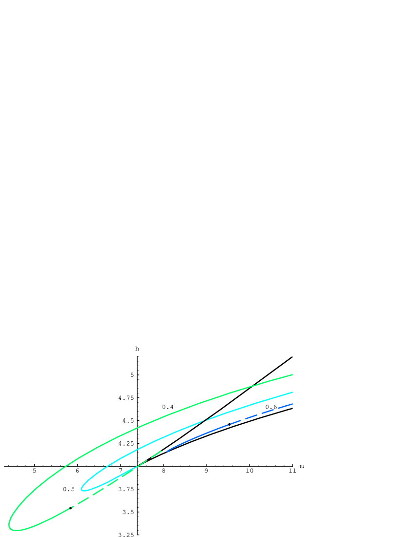
Figure 1: Loci of fold and Hopf bifurcation in the parametric plane $h,m$. The three Hopf curves correspond to $g=$ 0.4, 0.5 and 0.6. Solid grey lines show the supercritical, and dashed lines, the subcritical bifurcation. Outside the cusped region, the unique stationary state suffers oscillatory instability within the loop of the Hopf bifurcation locus. Within the cusped region, there are three stationary states, of which two, lying on the upper and lower folds of the solution manifold, may be stable. The solutions on the upper fold are unstable below the Hopf bifurcation line.

Figure 2: The stability boundary in the plane $(g_{0},y_{0})$, separating the regions of subcritical and supercritical Hopf bifurcation. The unphysical part of the curve below the boundary of positive frequency is shown by a dashed line. The solid circle at $g_{0}=0.5,y_{0}=2$ marks the double zero point.

References

- [1] Guckenheimer, J. & Holmes, P. [1983] Nonlinear Oscillations, Dynamical Systems and Bifurcations of Vector Fields, Springer, Berlin.
- [2] Guckenheimer, J., Myers, M. & Sturmfels, B. [1996] Computing Hopf Bifurcations I, SIAM J. Num. Anal., in press.
- [3] Haken, H. [1987] Advanced Synergetics, Springer, Berlin.
- [4] Hale, J.K. & Koçak, H. [1991] Dynamics and Bifurcations, Springer, Berlin.
- [5] Lorenz, E. N. [1963] Deterministic Nonperiodic Flow, J. Atmospheric Sci. 20, 130.
- [6] Nicolis, G. & Prigogine, I. [1977] Self-organization in Nonequilibrium Systems, from Dissipating Structures to Order through Fluctuations, Wiley, New York.
- [7] Pismen, L.M. [1986] Methods of Singularity Theory in the Analysis of Dynamics of Reactive Systems, Lectures in Applied Mathematics, 24, part 2, p. 175, AMS.
- [8] Pismen, L.M., Rubinstein, B.Y. & Velarde, M.G. [1996] On Automated Derivation of Amplitude Equations in Nonlinear Bifurcation Problems, Int. J. Bif. Chaos, in press.
- [9] Uppal, A., Ray, W.H. & Poore, A.B. [1974] On the Dynamic Behavior of Continuous Stirred Tank Reactors, Chem. Eng. Sci. 29, 967.
- [10] Wolfram, S. [1991] Mathematica. A System for Doing Mathematics by Computer, 2nd ed., Addison – Wesley.