Nonadiabatic couplings and incipience of quantum chaos

Abstract

The quantization of the electronic two site system interacting with a vibration is considered by using as the integrable reference system the decoupled oscillators resulting from the adiabatic approximation. A specific Bloch projection method is applied which demonstrates how besides some regular regions in the fine structure of the spectrum and the associated eigenvectors irregularities appear when passing from the low to the high coupling case. At the same time even for strong coupling some of the regular structure of the spectrum rooted in the adiabatic potentials is kept intact justifying the classification of this situation as incipience of quantum chaos.

January 19, 1996

1 Introduction

Nonadiabatic couplings are essential to derive from the basic idea of the Born - Oppenheimer (BO) approximation a rigorous procedure and were introduced already by Born itself in order to put this approximation into a complete scheme [1]. As has recently become clear these couplings can be the source of nonintegrability and produce chaotic behaviour in the dynamics of systems treated in the mixed quantum - classical description (see e. g. [2, 3]). In this paper the manifestations of these couplings in the structure of the energy spectrum and the eigenvectors are considered for a fully quantized electronic - vibronic coupled system which displays chaotic dynamics in the mixed description [4]. The electronic subsystem is a two site system (dimer) represented by a two state basis, whereas for the vibronic subsystem a large number of basis states has been taken into account in order to meet the basic condition behind the BO approximation for dividing the total system into fast (electronic) and slow (vibronic) subsystems. Furthermore this is the situation when one expects the best correspondence when passing for the slow subsystem from the classical approximation to the quantum description. This last step completes the quantization according to the BO scheme and is of general interest in the context of the problem how chaos in systems with a mixed quantum - classical description is reflected in their spectrum after full quantization is performed [5].

The problem, which signatures of chaos the eigenvalue spectrum displays in systems with a finite number of electronic quantum states (representable as spin states) coupled to a vibration (boson field) has already been addressed in the early papers on quantum chaos (see [6, 7]). The result of this research was that despite some irregularities in the spectrum the level spacing statistics is mostly regular. Here we demonstrate for one explicit system of this class, namely the excitonic - vibronic coupled dimer (for details of the model see [4]), that in fact in this kind of systems one can follow how the irregularities in the eigenvalue spectrum and the associated eigenstates appear through patterns of growing complexity when a characteristic coupling parameter is increased. Hence these systems have to be placed between systems with regular and completely irregular spectra. The appearance of irregularities in the eigenvalue spectrum or incipience of quantum chaos was recently reported for the spectrum of the spin - boson Hamiltonian with the Jaynes - Cummings model as the integrable reference system [8]. Here we use a different approach focussing on the properties of the spectrum for oscillator frequencies small compared to the electronic transfer matrix element, because we consider as the integrable reference system the decoupled oscillators resulting from the adiabatic approximation. Correspondingly we select a parameter region very much different from [8]. This approach deserves particular attention since the widespread use of the adiabatic approximation makes the problem, how the spectrum is modified when a rigorous scheme including nonadiabatic couplings is applied and which are the differences in this respect between regular and chaotic systems very significant. Using the the excitonic - vibronic coupled dimer as an example we show that for the low coupling case the overall structure of the spectrum of the electronic - vibronic system can easily be understood from the adiabatic approximation. For higher coupling it is possible to observe how the mixing of the adiabatic sequences of levels results in the appearance of irregularities in the spectrum. In particular, from our approach it is evident that this ”birth” of irregularities, or incipience of quantum chaos, is induced by the nonadiabatic couplings in the region of the energetic overlap of the adiabatic potentials.

2 The Model

The electronic two site system coupled to a vibration is represented in the form

$$H=\pmatrix{\epsilon+{\gamma\over\sqrt{2}}\,q+U(q)&V\cr V&\epsilon-{\gamma\over\sqrt{2}}\,q+U(q)}+{\hat{T}}\,{\mathbf{I}}$$ (1)

where $\epsilon$ is the electronic site energy (symmetric dimer), $V$ the transfer matrix element between the sites, $q$ the oscillator coordinate, $U(q)$ its potential energy and $\gamma$ the coupling constant. $\hat{T}$ and $\mathbf{I}$ are the kinetic energy of the oscillator and the identity operator in a two state basis respectively. We set $\hbar=1$ and $\epsilon=0$.

The separate diagonalization of the first term in (1) yields as eigenvalues the adiabatic potentials

$$U^{\pm}_{\mathrm{a}d}(q)=\pm\sqrt{V^{2}+{{\gamma^{2}}\over 2}q^{2}}+U(q),$$ (2)

which display the splitting into the bonding (-) and antibonding (+) branches. In the adiabatic approximation these branches are considered as independent and the action of $\hat{T}$ is restricted to the corresponding subspaces. The full action of $\hat{T}$ includes the nonadiabatic couplings resulting in a mixing of the adiabatic eigenstates.

We investigated the fine structure of the spectrum and the the associated eigenstates of the Hamiltonian (1) including the nonadiabatic couplings for a harmonic potential $U(q)=(\omega^{2}/2)q^{2}$. The problem depends on two dimensionless parameters which were chosen as $r={\omega\over 2V}$ and $p={\gamma^{2}\over 2V\omega^{2}}$. The parameter $p$ represents the coupling in these units. An important point is that $p$ appears in form of the product $\sqrt{p}r$ in the off diagonal elements of the Hamiltonian matrix in the adiabatic basis, i. e. the nonadiabatic mixing is governed by the effective coupling $\sqrt{p}r$. Below $p$ is used as the second independent parameter, however, because this parameter controls the bifurcation of the stationary states associated with the bonding branch $U^{-}_{\mathrm{a}d}(q)$ and the dynamics of the model in the mixed quantum - classical description [4].

In order to establish the influence of the nonadiabatic couplings the eigenvalue spectrum in the adiabatic approximation has to be found. For the determination of the adiabatic branches we use that in the region of highly excited oscillator states, i. e. large quantum numbers, the approximation

$$U_{\mathrm{ad}}^{\pm}(q)\sim\pm{\gamma\over\sqrt{2}}|q|+U(q)=-{\omega^{2}\over 2}q_{0}^{2}+{\omega^{2}\over 2}(|q|\pm q_{0})^{2},\hskip 14.22636ptq_{0}={\gamma\over\sqrt{2}\omega^{2}}$$ (3)

can be used in (2), which captures both the splitting of the ground state into two degenerate minima and the asymptotic dependences on $q$ for large $q$. The branch $U_{\mathrm{ad}}^{-}$ represents the textbook problem of the double oscillator [9]. Its solution by parabolic cylinder functions can easily be modified to include the branch $U_{\mathrm{ad}}^{+}$ as well. Using the asymptotic expansion of the parabolic cylinder functions one obtains the following expression for the spacings between adjacent levels with the same parity, $\Delta E_{i}=E_{i+1}-E_{i}$ in the adiabatic approximation and for large $E_{i}$

$$\Delta E_{i}^{\pm}\sim{2r\over 1\mp{1/\pi\sqrt{p/E_{i}^{\pm}}}},$$ (4)

where $\pm$ ($\mp$ in the denominator) refer to the upper / lower part of the adiabatic potentials (2), (3).

3 Analysis of the Numerical Results

We performed a numerical diagonalization of the Hamiltonian (1) in a finite electronic - oscillator basis including the nonadiabatic couplings. The adiabatic case of small oscillator frequencies compared to the electronic matrix element $V$ was considered, i. e. $r\ll 1$. Then, in order to reach the region of energetic overlap of the two adiabatic level sequences where the nonadiabatic mixing occurs, a relatively large number of vibrational basis states has to be taken into account (in our case of the order of $10^{3}$).

The Hamiltonian (1) commutes with the total parity operator which exchanges the sites of the dimer and reflects the oscillator coordinate. Correspondingly the eigenstates are characterized by their parity. Below the results for the positive parity states are presented, the results for negative parity are similar.

Analyzing the eigenvalues and associated eigenvectors we applied a specific projection method projecting the eigenstates onto the Bloch sphere of the electronic subsystem. This projection is performed by calculating for each eigenstate the expression $x_{i}^{(\nu)}=c^{(i)*}_{\nu,1}c_{\nu,2}^{(i)}+c_{\nu,1}^{(i)}c_{\nu,2}^{(i)*}$, where the $c_{\nu,s}^{(i)}$ are the expansion coefficients of the eigenvector $i$ in the combined electronic - vibronic basis, the indices $s=1,2$ refer to the electronic two site basis and $\nu=1,\dots N$ to the vibrational basis states. $N$ is the total number of vibrational basis functions, which are taken as harmonic oscillator eigenstates. Then the sum $x_{i}=\sum_{\nu}x^{(\nu)}_{i}$ over all vibrational states is calculated which gives the average Bloch variable $x_{i}$ associated with each eigenstate. $x$ is a useful quantity to distinguish between the mainly bonding or antibonding nature of the states in the electronic subspace associated with the two branches of the adiabatic potential (2) (for the details of the Bloch representation of the dimer see [4]). We recall that $x=+1$ and $x=-1$ for a pure bonding or antibonding state, respectively. Below we use the sign of $x$ as an indicator of the mainly bonding or antibonding nature of the eigenstates.

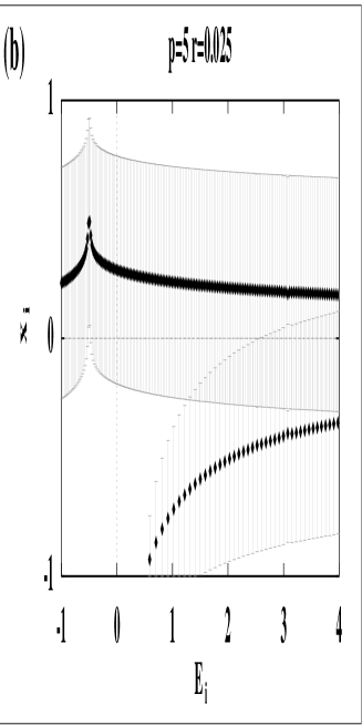
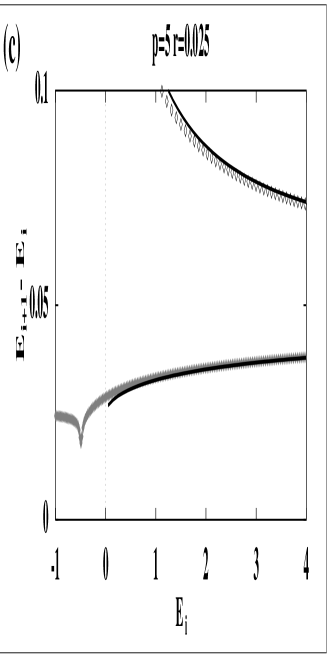
Figure 1: Analysis of the spectrum for positive parity states in the low coupling case $p=5$ and $r=0.025$, all energies are in units of $2V$: (a) Spacings $\Delta E_{i}$ between adjacent levels as a function of $E_{i}$ (b) Expectation values (diamonds) and variances (bars) of the Bloch variable $x_{i}$ associated with each eigenstate. Two separate strands can be resolved. (c) Resolution of the spacings shown in (a) according to the sign of the Bloch variable $x_{i}$ into two strands. The spacings between levels with $x_{i}>0$ and $x_{i}<0$ are shown with full and empty diamonds, respectively. The scatter of $\Delta E_{i}$ values in the region of overlap of the adiabatic potentials is completely resolved into two monotonic dependences close to the level spacings of the adiabatic potentials (4) which are shown as full lines.

A standard representation to resolve the fine structure of the spectrum is the dependence of the energetic difference of two subsequent eigenvalues $\Delta E_{i}=E_{i+1}-E_{i}$, i. e. the level spacing, on the position of the eigenvalues $E_{i}$ itself. In Fig. 1(a) such a dependence is shown for the dimensionless coupling strength $p=5$ and $r=0.025$ (effective coupling $\sqrt{p}r\sim 0.06$). In the energy region below $E=0.5$ only the lower adiabatic potential which has a double well structure for the given parameters contributes to the spectrum. Consequently, the spectrum is regular and the spacings between consecutive energy levels show a smooth dependence on the energy with a cusp marking the saddle point of the double well. For energies above the minimum of the second adiabatic potential, in addition to the points on the smooth curve in the $\Delta E_{i}(E_{i})$ plot, which is still visible, we find points irregularly scattered below this curve. However, this irregularity is merely due to a superposition of the adiabatic level sequences which for this low coupling case interact only weakly. For assigning the individual levels to the two adiabatic ladders we have employed the projection of the associated eigenvectors onto the Bloch sphere mentioned above. In Fig. 1(b) the expectation value of the Bloch $x$ - variable and its variance are displayed. It is evident that the eigenvectors can be approximately divided into two groups which are the analogue to the strands introduced in [8]. In Fig. 1(c) only the spacings between eigenvalues belonging to the same group have been plotted. It is obvious that the spectrum has been resolved into two smooth dependences which are very close to the approximate level spacings of the adiabatic potentials (4) shown as full lines in Fig. 1(c). We conclude, that the spectrum for this low coupling case can be well understood in the adiabatic approximation.

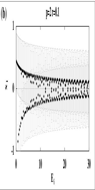
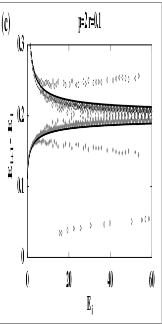
Figure 2: Analysis of the spectrum for $p=2$ and $r=0.1$ as in Fig. 1. (c) The majority of spacings for large $E$ are close to the full lines which mark the adiabatic level spacings (4), but others are far off. The parameters chosen are in the region of the gradual breakdown of the adiabatic approximation and mark the limit of applicability of the Bloch projection method for a separation of the spectrum into strands.

In the set of figs. 2(a)-(c) the same type of dependences as in figs. 1(a)-(c) are displayed for the parameters $p=2$ and $r=0.1$ giving $\sqrt{p}r\sim 0.14$ which is above the effective coupling of Fig. 1. However, due to the higher value of $r$, in Fig. 2 a much larger energy interval is required to display the same number of eigenstates. The functions (4) corresponding to the adiabatic potentials (3) are again shown as lines in Fig. 2(c). It is seen that for the given coupling value most of the spacings are still reproduced by the integrable reference oscillators of the adiabatic approximation. At the same time a substantial part of the data is displaced from the adiabatic dependences indicating that there are pairs of states with mainly bonding or antibonding nature completely outside their adiabatic strands, i. e. due to the nonadiabatic mixing the spectrum cannot be described as a superposition of two independent sequences.

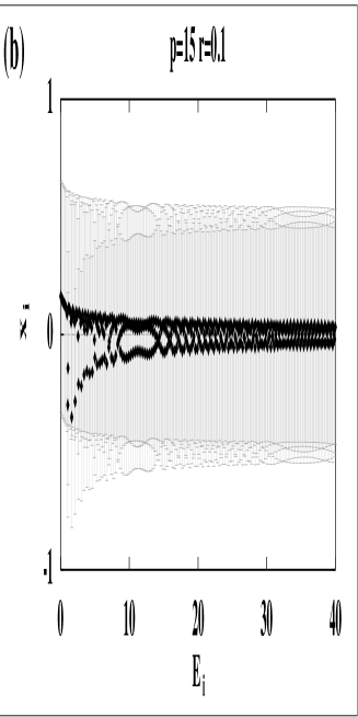
Figure 3: Analysis of the spectrum for $p=15$ and $r=0.1$ as in parts (a) and (b) of Fig. (1).

The effect of stronger mixing of the bonding and antibonding components in the eigenstates for a still higher coupling is evident from figs. 3(a)-(b), where the parameters $p=15$ and $r=0.1$, the effective coupling being $\sqrt{p}r\sim 0.39$, were used. The spacings of Fig. 3(a) show regular regions interrupted by regions with irregularly scattered data. The average Bloch variables have now merged into a band located around the $x=0$ line (Fig. 3(b)), i. e. a reasonable distinction between the eigenstates as mainly bonding and antibonding is not possible any more (compare to Fig. 2(b) where this distinction can still be made) and there is no separation in the fine structure of the spectrum, such as shown in Fig. 2(c) possible. As in the spacings data there are regular regions interrupted by irregular parts in the transition between the upper and lower boundaries of the band of Bloch variables. The band of average Bloch variables is now entirely embedded into the variances which provide additional information about the stronger degree of mixing between the bonding and antibonding components of eigenstates, compare figs. 1(b)-3(b). This comparison demonstrates that with increasing coupling the characterization of the eigenstates by quantities other than the energy, such as the Bloch variables becomes increasingly meaningless.

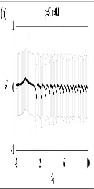
Figure 4: Analysis of the spectrum for $p=50$ and $r=0.1$ as in parts (a) and (b) of Fig. (1).

Finally we turn to the examination of a representative high coupling case. In Fig. 4 the dependences analogous to Fig. 3 are represented for the parameter values $p=50$ and $r=0.1$, the effective coupling being $\sqrt{p}r\sim 0.71$. Comparing Fig. 4(a) with the figs. 2(a) and 3(a) it is seen that the lower boundary of the spacing data is shifted to higher values, i. e. there is a clear tendency of repulsion between all the pairs of neighbouring levels with increasing nonadiabatic coupling. This formation of avoided crossings in the spectrum is a clear signature of the classical chaos in the quantum spectrum (see e. g.  [11]). As in Fig. 3(b) the average Bloch variables remain localized in a band around the $x=0$ line, this band being embedded in a broad band of variances (Fig. 4(b)).

Although our analysis demonstrates how irregularities in the spectrum for increasing coupling strength appear, not all regular structures have disappeared. In particular, the smooth dependence of $\Delta E_{i}$ on $E_{i}$ associated with the bonding branch of the adiabatic potential and observed for energies below the onset of the mixing of the adiabatic sequences, is still visible for higher energies by a thought continuation of this line into the mixing region. This is clearly observed for all the coupling cases in the figs. 1(a)-3(a) and this feature is still present even for the strong coupling of Fig. 4(a). There, however, the lower boundary of the spacings data has been dissolved in contrast to the previous figures.

We note that in the high coupling case of Fig. 4 the energy interval for which correct numerical eigenvalues are available is smaller than in figs. 2 and 3. This is due to the stronger mixing of the basis states used for the numerical diagonalization which makes the finite basis size perceptible at lower energies. Beside this problem we mention that from the point of view of a spectrum formation starting from adiabatic eigenstates the region with relevant nonadiabatic mixing shifts to higher energies with increasing coupling. This is due to the steepening of the upper branch of the adiabatic potential (2) which increases the energy of the associated states. Correspondingly for increasing coupling one has to pass to higher energies in order to observe the effect of the nonadiabtic mixing on the spectrum. Hence any finite basis used in the numerical diagonalization restricts both the accessible energy interval and the amount of numerical data in the mixing region for the strong coupling case.

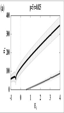
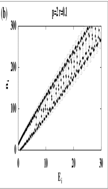
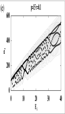
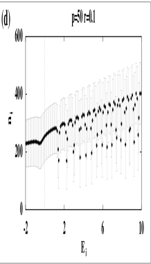
Figure 5: Expectation values (diamonds) and variances (bars) of the degree of vibronic excitation $n_{i}$ associated with each eigenstate. The parameters of part (a)-(d) correspond to those of figs. 1-4, respectively, and are given above the plots.

The analysis of the eigenstates is complemented by considering the degree of excitation in the vibronic subspace in form of the average number of vibrational quanta $n_{i}$ associated with each eigenstate $n_{i}=\sum_{\nu,s}\nu|c_{\nu,s}^{(i)}|^{2}$. The corresponding data for $n_{i}$ and its variances as a function of the energy are shown in figs. 5(a)-(d) for the same parameters as used before. In Fig. 5(a) the number $n_{i}$ and its variance are displayed for the low coupling case corresponding to Fig. 1. As for the Bloch variables in Fig. 1(b) the resolution into two well resolved strands is clearly seen. The strands demonstrate the splitting of the degree of vibrational excitation of the eigenstates into well separated high and low energy parts corresponding to vibronic wave functions with a large and small number of nodes, respectively. The presence of two well resolved species of states in the two site excitonic - vibronic system for certain parameter values and their possible experimental consequences were reported in a number of recent papers (see [10] and references therein). We note that this feature is also obtained by the Bloch projection method, i. e. figs. 1(b) and 5(a) are in fact complementary. The figs.5(b)-(d) show the irregularities arising in the distribution of vibrational excitation between the eigenstates. Increasing the coupling the growing disorder in the spectrum is complemented by transitions between states with low and high levels of vibrational excitation as is evident from figs. 5(b) and 5(c). In the level of vibrational excitation one now finds patterns showing growing complexity in the transitions between states of low and high vibrational excitation. We note that the pattern of Fig. 5(c) must be considered with some caution: in this case the variances are much broader than in the case of Fig. 5(b). Finally in the high coupling case presented in Fig. 5(d) the lower part of the $n$ - distribution has become irregular, though there is clearly an upper limit in the level of vibrational excitation visible. As in Fig. 4(a) this structure can again be traced back to the bonding branch of the adiabatic potential, i. e. some regular features remain.

Summarizing the result of the Bloch projection method we can show by this method that for the low coupling case some apparent irregularities in the spectrum can be resolved and the spectrum in fact be interpreted as an approximate superposition of adiabatic level sequences. For higher couplings this method shows that the Bloch variables merge into a band indicating that a separation of the spectrum into adiabatic sequences is not possible any more. Considering the distribution of vibrational excitation between the eigenstates we find the same behaviour, i. e. both views are in fact complementary. The Bloch projection seems however simpler since it employs a projection on the low dimensional space of two bonding/antibonding states. The Bloch projection allows to follow how the genuine irregularities in the spectrum appear together with a destruction of the classification of eigenstates such as bonding and antibonding according to criteria other than their energy. An essential point is that for the coupled excitonic - vibronic system the formation of irregularities in spectrum and associated eigenstates is not complete: some of the regular structures are conserved. This feature justifies the classification of this situation as incipience of quantum chaos.

4 Conclusions

1. The main aim of this paper was to show how irregularities in the spectrum and associated eigenvectors of the fully quantized electronic two site system coupled to a vibration appear when a characteristic coupling parameter is increased. The considered system belongs to the class of models which show regular and chaotic dynamics in the mixed quantum - classical description when a stepwise quantization is applied treating the electronic subsystem in the quantum but the vibronic subsystem in the classical context [4]. Hence it is natural to ask for the ”fingerprints” of the dynamical chaos in the mixed description after full quantization is performed. Considering the fully quantized system we employed the adiabatic approximation as a standard way to define an integrable reference system and used the nonadiabatic couplings as the parameter to control the degree of nonintegrability and resulting spectral irregularities. In agreement with earlier findings [6, 7] for this type of system our results show that spectral irregularities and in particular avoided crossings, which are a signature of dynamical chaos, indeed appear, but do not develop into fluctuations of the kind one would expect from the standard examples of quantum chaos when quantizing a classically chaotic system results in spectral fluctuations characterized by universal statistics and random matrix theory. Increasing the nonadiabatic couplings we rather find a transition like behaviour characterized by the birth of spectral irregularities and growing disorder in the characterization of eigenstates. This growing disorder in the eigenstates proceeds through the destruction of regular patterns and shows how distinction criteria of eigenstates other than their energy such as provided by the Bloch projection or the level of vibrational excitation are lost.

2. Referring to the specific way in which the spectral structures associated with the Born - Oppenheimer approximation are dissolved when the characteristic coupling - the nonadiabatic mixing of the integrable oscillators of this approximation - is increased, we find that the mixture of both residual regular structure and disordered parts makes the spectrum in a sense unique. Even for large coupling the spectrum still contains the regular spacing dependence rooted in the adiabatic approximation and irregular parts scattered around it. In our view this situation can be best described as incipience of quantum chaos, which is in line with recent findings for the same kind of system viewed from spin - boson coupled systems in an another parameter region [8]. Our results show the specific way in which this incipience of quantum chaos develops by the nonadiabatic coupling of the integrable reference oscillators of the adiabatic approximation.

3. Finally we comment on the reason why the present system is of the incipience type thereby pointing to other more complex situations when the incipience case can be expected to pass into the situation of fully developed spectral fluctuations after complete quantization. From the view of the adiabatic approximation, there are obviously two points to mention in order to obtain a more complex system: i) to increase the number of coupled adiabatic reference oscillators, i. e. the dimension of the Hilbert space of the fast subsystem and ii) to increase the degree of nonlinearity of the reference oscillators which are coupled. As viewed from these points the present system is obviously of the simplest form, there are two basis states of the fast subsystem and the degree of nonlinearity of the adiabatic potentials (2), (3) is mild. We conclude that the increase in the number of coupled adiabatic reference systems and/or the degree of their nonlinearity is essential to further investigate the connection between chaos of systems treated in the mixed quantum - classical description of the first step and the signatures of this chaos after full quantization is performed in the second step of the Born - Oppenheimer procedure.

References

- [1] Born, M., Huang, K.: ”Dynamical Theory of Crystal Lattices”, Oxford, Clarendon Press, 1954. Appendix VIII
- [2] Bulgac, A., Kusnezov, D.: Chaos, Solitons & Fractals 5, 1051 (1995)
- [3] Blümel, R., Esser, B.: Phys. Rev. Lett. 72, 3658 (1994)
- [4] Esser, B., Schanz, H.: Z. Phys. B 96, 553 (1995)
- [5] Blümel, R., Esser, B.: Z. Phys. B 98, 119 (1995)
- [6] Graham, R., Höhnerbach, M.: Z. Phys. B 57, 233 (1984)
- [7] Kus, M.: Phys. Rev. Lett. 54, 1343 (1985)
- [8] Cibils, M., Cuche, Y., Müller, G.: Z. Phys. B 97, 565 (1995)
- [9] Merzbacher, E.: ”Quantum mechanics”, New York, J. Wiley & Sons 1970, Chapter 5
- [10] Sonnek, M., Eiermann, H., Wagner, M.: Phys. Rev. B 51, 905 (1995)
- [11] Haake, F.: ”Quantum signatures of chaos”, Berlin, Heidelberg, New York, Springer 1991