The effect of small-scale forcing on large-scale structures
in two-dimensional flows

Abstract

The effect of small scale forcing on large scale structures in $\beta$-plane two-dimensional (2D) turbulence is studied using long-term direct numerical simulations (DNS). We find that nonlinear effects remain strong at all times and for all scales and establish an inverse energy cascade that extends to the largest scales available in the system. The large scale flow develops strong spectral anisotropy: $k^{-5/3}$ Kolmogorov scaling holds for almost all $\phi$, $\phi=\arctan(k_{y}/k_{x})$, except in the small vicinity of $k_{x}=0$, where Rhines’s $k^{-5}$ scaling prevails. Due to the $k^{-5}$ scaling, the spectral evolution of $\beta$-plane turbulence becomes extremely slow which, perhaps, explains why this scaling law has never before been observed in DNS. Simulations with different values of $\beta$ indicate that the $\beta$-effect diminishes at small scales where the flow is nearly isotropic. Thus, for simulations of $\beta$-plane turbulence forced at small scales sufficiently removed from the scales where $\beta$-effect is strong, large eddy simulation (LES) can be used. A subgrid scale (SGS) parameterization for such LES must account for the small scale forcing that is not explicitly resolved and correctly accommodate two inviscid conservation laws, viz. energy and enstrophy. This requirement gives rise to a new anisotropic stabilized negative viscosity (SNV) SGS representation which is discussed in the context of LES of isotropic 2D turbulence.

1 Introduction

Turbulent flows subjected to differential rotation develop spectral anisotropy. Understanding and modeling such flows present a major theoretical and experimental challenge, mainly due to their geophysical, astrophysical and plasma physics importance. The simplest two-dimensional system of this kind describes the flow of a thin layer of homogeneous fluid on the surface of a rotating sphere. Such flows are governed by the barotropic vorticity equation in the $\beta$-plane approximation in which the fluid moves in tangential planes [1],

$${\partial\zeta\over\partial t}+{\partial\left(\nabla^{-2}\zeta,\zeta\right)\over\partial(x,y)}+\beta{\partial\over\partial x}\left(\nabla^{-2}\zeta\right)=\nu_{o}\nabla^{2}\zeta+\xi.$$ (1)

Here, $\zeta$ is the fluid vorticity, $\nu_{o}$ is the molecular viscosity, and $\xi$ is the forcing; $x$ and $y$ are directed eastward and northward, respectively.

The constant $\beta$ is the background vorticity gradient describing the latitudinal variation of the normal component of the Coriolis parameter, $f=f_{0}+\beta y$. Considering the energy transfer subrange typical of classical isotropic two-dimensional turbulence [2, 3], we assume that the forcing $\xi$ is concentrated around some high wave number $k_{\xi}$ and is random, zero-mean, Gaussian and white noise in time with the correlation function

$$\langle\xi({\bf k},t)\,\xi({\bf k^{\prime}},t^{\prime})\rangle=8\pi\,\eta\,\delta(k^{2}-k_{\xi}^{2})\,\delta({\bf k}+{\bf k^{\prime}})\,\delta(t-t^{\prime}),$$ (2)

where $\langle\dots\rangle$ denotes ensemble average. Thus defined, the forcing $\xi$ supplies the system (1) with energy and enstrophy at rates $\int\langle|\xi({\bf k},t)|^{2}\rangle/k^{2}\,d{\bf k}/(2\pi)^{2}=\epsilon=\eta/k_{\xi}^{2}$ and $\int\langle|\xi({\bf k},t)|^{2}\rangle\,d{\bf k}/(2\pi)^{2}=\eta$, respectively. In the inviscid limit, the corresponding total energy and enstrophy vary in time as in the isotropic case, according to $E(t)=E(0)+\epsilon\,t$ and $\Omega(t)=\Omega(0)+\eta\,t$; the $\beta$-term does not enter these evolution laws explicitly.

In the linear limit with no forcing, Eq. (1) describes propagation of planetary, or Rossby waves with the dispersion relation

$$\omega_{\bf k}=-\beta k_{x}/k^{2},$$ (3)

while in the nonlinear limit without the $\beta$-term, this equation represents classical isotropic 2D turbulence. Thus, Eq. (1) describes the interaction of 2D turbulence and Rossby waves and is important for understanding of planetary scale geophysical processes.

The relative simplicity of Eq. (1) has placed it at the focal point of theoretical geophysical fluid dynamics, and much has been learned from this model. However, the large scale behavior of its solutions still remains controversial; their spectral evolution laws have not been well established, while the spectral anisotropy and the importance of nonlinearity have received insufficient attention in the existing literature. Here, using DNS, we address the problems of scaling laws and spectral anisotropy of $\beta$-plane turbulence governed by (1) and forced at small scales. In the next section, evolution and scaling laws of $\beta$-plane turbulence will be discussed. On relatively small scales the $\beta$-effect is small and the flow is nearly isotropic. On larger scales, the effect of the $\beta$-term becomes progressively stronger, and spectral anisotropy develops. Along with that, spectral evolution slows down considerably, compared to the isotropic case. As a result, prohibitively long integration time is required for low wavenumber modes to become excited even for relatively moderate resolution. To address this problem, LES of $\beta$-plane turbulence can be sought. In section 3, an eddy viscosity for such LES is calculated. This SGS representation includes negative Laplacian term that accounts for the unresolved small scale forcing and inverse cascade. Thus, this SGS representation gives rise to a stabilized negative viscosity (SNV) SGS parameterization [4]. In section 4, some results of the application of this SNV representation to isotropic 2D flows are presented. Finally, in section 5, we summarize our results and conclusions.

2 Evolution and Scaling Laws of $\beta$-Plane Turbulence

Preliminary asymptotic analysis of Eq. (1) reveals that as $k\to\infty$, the amplitude of the $\beta$-term decays as $k^{-1}\cos\phi~{}~{}[\phi=\arctan(k_{y}/k_{x})$], so that for large $k$, the $\beta$-effect is expected to be small and the system should behave mostly as isotropic 2D turbulence in the energy transfer subrange [2, 3, 5]. The energy spectrum defined as $E({\bf k},t)=2\pi\,\langle|\zeta({\bf k},t)|^{2}\rangle/k$, with $\int dk\int_{0}^{2\pi}E({\bf k},t)d\phi/(2\pi)=E(t)$ being the total energy, is nearly isotropic, $E({\bf k},t)\approx E(k,t)$, and Kolmo-gorov-like, i.e.

$$E_{K}(k)=C_{K}\,\epsilon^{2/3}\,k^{-5/3},$$ (4)

where $C_{K}$ is the Kolmogorov constant. On the other hand, Rossby waves dominate as $k\to 0$. Assuming that the energy spectrum in this limit is determined by $\beta$ and $k$ only, one finds, using dimensional considerations [6]

$$E_{R}(k)=C_{R}\,\beta^{2}\,k^{-5},$$ (5)

where $C_{R}$, by analogy to the Kolmogorov constant, can be referred to as the Rhines constant. For isotropic 2D turbulence, the estimate of the Kolmogorov constant $C_{K}$ from DNS and analytical theories of turbulence is about 6. On the other hand, the Rhines spectrum (5) has not been observed in DNS so far so that not only no estimate of $C_{R}$ is available, but even the very existence of the spectrum (5) has been in doubt.

Turbulence and waves have comparable effects when the eddy turnover time of isotropic 2D turbulence approaches the Rossby wave period, which occurs at a transitional wave number, $k_{t}(\phi)$,

$$k_{t}(\phi)=k_{\beta}\cos^{3/5}\phi,~{}~{}k_{\beta}=(\beta^{3}/\epsilon)^{1/5}.$$ (6)

The contour (6) in wavevector space has been termed “the dumb-bell shape” by Vallis and Maltrud [7]; earlier, a similar contour was called “lazy 8” by Holloway [8] in the context of $\beta$-plane flow predictability studies. According to [6], as $k\to k_{\beta}$, the inverse energy cascade slows down, and increasing spectral anisotropy facilitates preferential energy transfer into large scale structures with $k_{x}\to 0$, or zonal jets. This conceptual picture was further developed in later publications. In particular, Vallis and Maltrud [7] found that as $k\to k_{\beta}$, the dumb-bell shape becomes a barrier for turbulence energy. However, since the dumb-bell shape excludes the axis $k_{x}=0$, the inverse cascade can continue in the vicinity of $k_{x}=0$ facilitating the funneling of the energy into coherent structures corresponding to zonal flows. Rhines [6], Vallis and Maltrud [7], and Holloway [9] note that the spectral anisotropy induced by the $\beta$-term can be associated with the mechanism of generation and maintenance of zonal flows. Zonal structures are robust features of the simulations by Rhines [6], Vallis and Maltrud [7] and Panetta [10], as well as of the large scale Earth and planetary circulations. On the other hand, for $k<k_{\beta}$ one would expect that nonlinear transfer becomes relatively ineffective, and the flow regimes inside the dumb-bell shape are more prone to linear dynamics [11]. Although this assumption underlines some theories, it has not been thoroughly tested in DNS so far. Generally, processes at $k<k_{\beta}$ were avoided in the previous DNS of $\beta$-plane turbulence. Thus, not only could these processes not be properly resolved ($k_{\beta}$ usually did not exceed 20 or so), but the whole region $k<k_{\beta}$ was treated rather as an area of large scale energy dissipation due to linear (Ekman) drag or other factors.

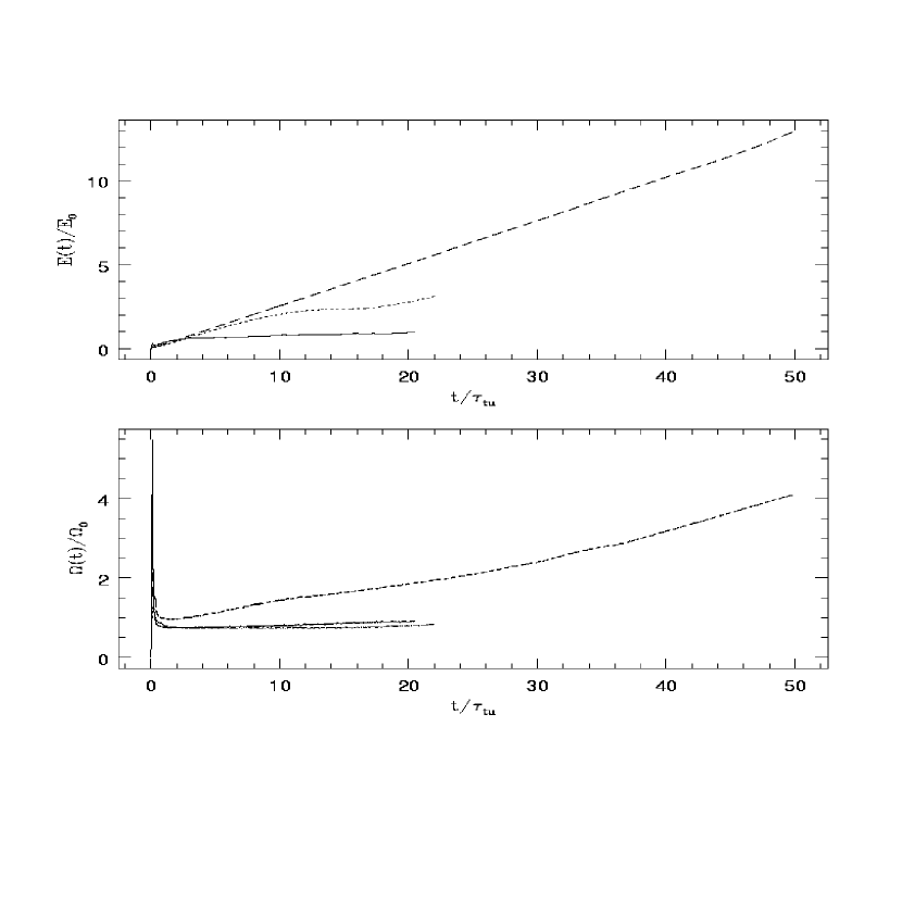
Figure 1: Evolution of total energy $E(t)$ (top) and enstrophy $\Omega(t)$ (bottom) for Cases 1, 2 and 3 (solid, dotted, and dashed lines, respectively).

In the present DNS, the processes at scales of the order of $k_{\beta}^{-1}$ and larger are of primary interest. These DNS employ a fully-dealiased pseudospectral Fourier method to solve Eq. (1) in a box $\{x,y\}\in[0,2\pi]\times[0,2\pi]$ with doubly periodic boundary conditions and zero initial data. The spatial resolution is $512^{2}$ and the 2/3 dealiasing rule is used. The time discretization is the same as in [12]. A hyperviscous term of the form $\nu_{S}\,(-1)^{p+1}\,\Delta^{p}\zeta+\nu_{L}\,(-1)^{q+1}\,\Delta^{-q}\zeta$ with $p=8$ and $q=5$ is introduced in (1) to ensure sharp energy removal from both small and large wave number modes. The forcing $\xi$ is represented by $\xi(k,t)=A_{\xi}\sigma_{k}(t)/\sqrt{\delta t}$ for $k\in[100,105]$ and is zero otherwise; here, $\delta t$ is the time step, and $\sigma_{k}(t)$ is a discrete and uncorrelated in time, Gaussian, random number with unit variance. Parameter setting for DNS reported here is: $\delta t=1.0$, $\nu_{L}=20.0$, $\nu_{S}=1.0\times 10^{-36}$, and $A_{\xi}=0.1$ which results in an energy injection rate of $\epsilon\approx 2.7\times 10^{-13}$. Results of three DNS, with $\beta$ = 0, $0.053$, and $0.3$, corresponding to $k_{\beta}$ = $0$, $56$, and $158$, respectively, are reported here and shown in Figs. 1–5. These cases will be referred to as Case 1, 2, and 3, respectively. All simulations were terminated when the energy reached the largest scales available in the computational box and condensation started affecting flow behavior at smaller scales [13, 14].

In Figure 1, we plot the evolution of total energy and enstrophy normalized by the corresponding values, $E_{0}$ and $\Omega_{0}$, of the steady state, isotropic ($\beta$ = 0) case. A striking feature is that increasing in $\beta$ causes increasing in computational time necessary for the effects of condensation to appear. For example, for $\beta$=0.3, the effect of large scale energy saturation becomes significant at about $t/\tau_{tu}\approx 50$, where $\tau_{tu}=2\pi/\sqrt{2E_{0}}$ is the large scale eddy turnover time of the steady state in the isotropic case. For comparison, in the corresponding isotropic DNS, the large scale energy condensate forms after only about $4\tau_{tu}$. In fact, the dramatic increase in computational time necessary for the energy to reach the lowest active modes in the system is the major factor hampering DNS of $\beta$-plane turbulence; the problem is exacerbated with increasing resolution. The reason why such a long integration time is required will be explained later.

The results plotted in Figure 1 show that in agreement with the conservation law, $E(t)$ exhibits linear in time growth. The analysis of mode-wise energy distribution (not shown here) indicates that increasingly longer time is required for saturation of the lower modes.

In Figures 2–4 we plot ${\bf k}$-dependent energy spectra averaged over small sectors $\pm\pi/12$ around $\phi=0$ and $\phi=\pi/2$. For Case 1, as expected, the spectrum is isotropic and Kolmogorov-like. When $\beta\neq 0$, spectral anisotropy develops. As Figs. 3 and 4 indicate, this anisotropy becomes more and more pronounced with increasing $\beta$. Although, as mentioned earlier, spectral evolution slows down with $\beta\neq 0$, spectral anisotropy develops relatively fast. In Figure 3 we show that for Case 2 with $k_{\xi}\in[100,105]$ and $k_{\beta}=56$, anisotropization begins at $t\approx\tau_{tu}$, while for Case 3 with $k_{\beta}=158$, anisotropization starts immediately. Long term integration indicates that in the direction $\phi=0$, or $k_{y}=0$, the Kolmogorov scaling (4) develops, while for the directions $\phi=\pm\pi/2$, a scaling similar to that of Rhines (5), $k_{y}^{-5}$, prevails. Compared to Fig. 3, Fig. 4 presents results of DNS with larger $\beta$, or larger $k_{\beta}$, leading to better resolution of the region $k<k_{\beta}$ and a more pronounced $k_{y}^{-5}$ spectrum. In Figure 5, we compare the compensated spectrum $E(k)\beta^{-2}k^{5}$ along $\phi=\pm\pi/2$ at the end of integration for Cases 2 and 3, i.e., for $t/\tau_{tu}=16.25$ and 30.12, respectively. An important conclusion that can be drawn from this comparison is that along $\phi=\pm\pi/2$, the energy spectrum scales with $\beta^{2}$. Combined with dimensional considerations, this result reaffirms the validity of the scaling (5) along $\phi=\pm\pi/2$. More detailed analysis of the anisotropic spectra reveals that the Kolmogorov $k^{-5/3}$ scaling holds for almost all directions $\phi$ except for the small vicinity of $\phi=\pm\pi/2$. It is important to emphasize that the inverse energy transfer does not cease for any direction and any $k\leq k_{\beta}$ and eventually extends to the largest scales available in the system. Rather than being a barrier, or even a soft barrier for the inverse energy cascade, $k_{\beta}$ only appears to be a threshold of spectral anisotropy. After the energy front reaches $k_{\beta}$, some readjustment of $C_{K}$ is observed; its value decreases from 6 to about 3. This points to the active energy exchange between the Kolmogorov and Rhines scaling regions facilitated by nonlinear interactions and to intensification of the Rhines’s flow regime at the expense of its Kolmogorov counterpart.

Generally, since the $k_{y}^{-5}$ spectrum is much steeper than the $k^{-5/3}$ spectrum, most of energy resides in sectors closely adjacent to $\phi=\pm\pi/2$, so that the angular-averaged energy spectrum also obeys Rhines’s $k^{-5}$ scaling (5). Therefore, the present DNS confirms Rhines’s arguments in [6]. Indeed, this is the first time that the $k^{-5}$ spectrum is observed in DNS. Our results also show why meaningful DNS of $\beta$-plane turbulence requires much longer integration times than the corresponding isotropic DNS. Indeed, from the total energy evolution law for both isotropic and $\beta$-plane turbulence, $E(t)\propto\epsilon t$, one estimates that the time required for the energy front to reach wave number $k$ is $t\propto E(t)/\epsilon$. For the same $\epsilon$, the ratio of these characteristic time scales, $t_{R}/t_{K}$, for Rhines and Kolmogorov spectra can be estimated from (4) and (5) by angular averaging and integrating corresponding energy spectra between $\infty$ and $k$ giving $t_{R}/t_{K}\propto(k_{\beta}/k)^{10/3}$. For Cases 2 and 3 and $k=15$, one finds that $t_{R}/t_{K}$ is of the order of 80 and 2500, respectively.

Here, further discussion of the physical meaning of $k_{\beta}$ given by (6) would be relevant. Other definitions of $k_{\beta}$ have been used in the literature interchangingly with (6) (see, for instance, [7]). One of those definitions is due to Rhines [6], $k_{\beta}=(\beta/2U)^{1/2}$, and another one is due to Holloway and Hendershott [15], $k_{\beta}=\beta/\zeta$. Here, $U$ is a characteristic velocity which can be identified with the square root of the total energy of the system, while $\zeta$ is a characteristic vorticity that can be identified with the square root of the total enstrophy of the system. For the $k^{-5}$ spectrum, it can be shown that, within numerical coefficients, both Rhines’s and Holloway and Hendershott’s definitions provide $k_{\beta}=k$, where $k$ is the smallest wavenumber attained by the energy front. Furthermore, taking into account the evolution law of $\beta$-plane turbulence, one can show that thus defined $k_{\beta}$ is time dependent, $k_{\beta}\sim t^{-1/4}$. Therefore, definitions (6) and those suggested by Rhines [6] and Holloway and Hendershott [15] characterize different processes in $\beta$-plane turbulence. While the former provides the stationary threshold separating the regions of nearly isotropic and strongly anisotropic, Rossby wave dominated turbulence, the latter pertain to the largest scales available in the system at any given time.

To better understand the anisotropy of the energy (or enstrophy) spectrum of $\beta$-plane turbulence, let us consider the enstrophy transfer function $\mathchar 29268\relax_{\Omega}({\bf k},t)$ derived from the enstrophy equation

$$\left[{\partial\over\partial t}+2\nu_{o}k^{2}\right]\Omega({\bf k},t)=\mathchar 29268\relax_{\Omega}({\bf k},t).$$ (7)

Here, $\Omega({\bf k},t)$ is vorticity correlation function, and $\mathchar 29268\relax_{\Omega}({\bf k},t)$ is given by

$$\mathchar 29268\relax_{\Omega}({\bf k},t)=2\pi k\int_{{\bf p}+{\bf q}={\bf k}}\frac{{\bf p}\times{\bf q}}{p^{2}}\langle\zeta({\bf p},t)\zeta({\bf q},t)\zeta(-{\bf k},t)\rangle\frac{d{\bf p}~{}d{\bf q}}{(2\pi)^{2}}.$$ (8)

Let us introduce a cutoff wavenumber $k_{c}$ separating explicit $(k<k_{c})$ and implicit, or SGS $(k>k_{c})$ modes and consider enstrophy exchange between all implicit modes and a given explicit mode ${\bf k}$ in the limit $t\to\infty$. Following [16], this exchange is denoted by $\mathchar 29268\relax_{\Omega}({\bf k}|k_{c})$ and is obtained from (8) by extending integration only over all such triangles $({\bf k,~{}p,~{}q})$ that $p$ and/or $q$ are greater than $k_{c}$.

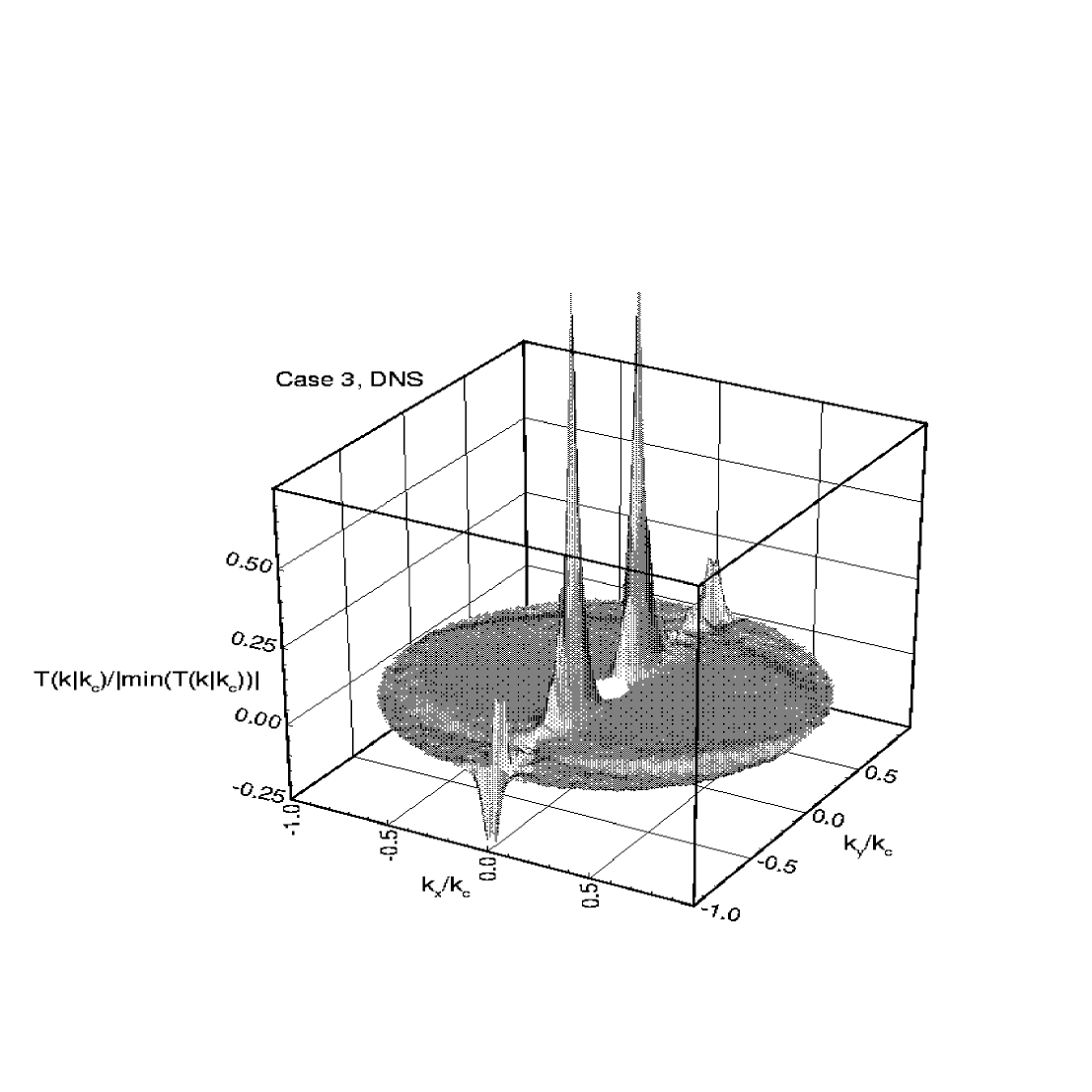
Figure 6: Spectral energy transfer, $\mathchar 29268\relax_{E}({\bf k}|k_{c})$, for $k_{c}=50$.

In Figure 6, we plot the anisotropic energy transfer $\mathchar 29268\relax_{E}({\bf k}|k_{c})$ derived from the corresponding enstrophy transfer $\mathchar 29268\relax_{\Omega}({\bf k}|k_{c})$ for Case 3 with $k_{c}=50$. Obviously, $\mathchar 29268\relax_{E}({\bf k}|k_{c})$ describes energy transfer from all SGS modes with $k>k_{c}$ to an explicit mode with the wavenumber ${\bf k}$, $k<k_{c}$. As in [12], this energy transfer function was calculated here directly from DNS results. Consistently with the isotropic case [12], $\mathchar 29268\relax_{E}({\bf k}|k_{c})$ develops a cusp at $k\to k_{c}$. As $k\to 0$, strong anisotropy prevails, and most of the energy is funneled into the sectors adjacent to $\phi=\pm\pi/2$. On the one hand, the modes with small $k_{x}$ carry most of the energy; on the other, they allow for weak $x$-dependency of the flow field, thus maintaining nontrivial nonlinearity which in turn sustains anisotropic transfer. Thus, the modes with small $k_{x}$ correspond to nearly one-dimensional, zonal structures, or jets. Such structures are clearly seen in an instantaneous snapshot of the vorticity field in physical space at $t=39.6\tau_{tu}$ for Case 3 as plotted in Fig. 7; these jets have also been a robust feature of earlier simulations [7, 10]. The observation that can be made based upon the present DNS is that the number of jets is very close to the minimal excited wavenumber in the energy spectrum; there is no obvious linkage between the number of jets and $k_{\beta}$.

The zonally-averaged velocity component $U(y,t)$ is plotted in Fig. 8 for Case 3. Initially, the jets were nearly symmetric with respect to the reflection $y\rightarrow-y$. By $t=39.6\tau_{tu}$, the zonal jets develop strong asymmetry; as also observed in [7], eastward jets are sharp and narrow while westward jets are smooth and wide. It is important to know whether or not these jets are stable with respect to perturbations with nonzero $k_{x}$. Although the velocity field is time-dependent, the meridional motions are rather slow compared to zonal flows. In this case, the Rayleigh–Kuo inviscid stability criterion generalized for $\beta\neq 0$ requires that the profile $U(y,t)-\beta\ y^{2}/2$ has no inflection points for the flow to be linearly stable. Examination of the second derivative $U_{yy}(y,t)$ shown in Fig. 8 demonstrates that the Rayleigh–Kuo criterion $U_{yy}(y,t)-\beta\neq 0$ does hold, which also agrees with the results in [7]. Furthermore, as time advances, the profile of $U_{yy}(y,t)$ develops large negative peaks thus ensuring linear stability at later times. As long as the effect of the large scale drag remains small, excitation of progressively smaller wavenumber modes leads to a diminishing number of jets, in agreement with other simulations [10]. It is interesting to note that in models of barotropic flows on a $\beta$-plane with externally imposed mean flow $U$, the difference $\beta_{e}=\beta-U_{yy}$ may decrease to zero or even become negative. The sign of $\beta_{e}$ is related to interaction between the critical layer and Rossby waves and may point to absorption ($\beta_{e}>0$), perfect reflection ($\beta_{e}=0$), or over-reflection ($\beta_{e}<0$) of Rossby waves by the critical layer (for more details, see [17, 18, 19, 20, 21]). In the present DNS, as well as in the previous studies by Vallis and Maltrud [7], the mean flow $U$ is generated and sustained by small scale random forcing, while $\beta_{e}$ is always positive.

In summary, it is useful to highlight the peculiarities caused by the nonlinear terms in barotropic vorticity equation on a $\beta$-plane. Although the $\beta$-term does not enter the energy and enstrophy equations explicitly, it has a profound effect on the energy spectrum and spectral transfer. This effect is solely due to the nonlinearity of Eq. (1) which facilitates interaction between Rossby waves and vorticity modes. As a result, the energy spectrum and transfer develop strong anisotropy for $k<k_{\beta}$ while the inverse energy cascade extends to ever smaller $k$. Furthermore, inside the dumb-bell shape (6), where, by simple scaling considerations, the $\beta$-effect is expected to prevail, the energy spectrum is determined not by $\beta$ but by the presumably irrelevant parameter $\epsilon$. On the other hand, in the small sectors around $\phi=\pm\pi/2$ outside the dumb-bell shape naive considerations show that the $\beta$-term is vanishing [$\beta\partial_{x}\nabla^{-2}\zeta\to i\beta k_{x}k^{-2}\zeta\to 0$ as $k_{x}\to 0$ in (1)] and the mechanism of anisotropic inverse transfer funnels energy into zonal jets. In the present DNS we find that the zonal jets do indeed form, but the effect of the $\beta$-term does not diminish by any means: the spectrum of energy in the regions $\phi\to\pm\pi/2$ is determined by $\beta$.

The possibility of energy transfer from Rossby waves to zonal flows has long been discussed in the literature and by no means is a trivial matter. Straightforward generalization of the Fjortoft theorem [22] shows that a resonant triad of wavevectors one of which is aligned with the axis $y$ does not allow for direct energy transfer into zonal flows. However, the vector with $k_{x}=0$ facilitates energy exchange between the other two vectors - members of the triad. This fact was proved in [23] in much more general way; it was shown that the coupling coefficient is zero for any such triad that $k_{x}=0$ for one of the vectors. Later, Newell [24] showed that Rossby waves can transfer energy into zonal flows through a sideband resonance mechanism or through a quartet resonance. Reinforcing this result, the present DNS indicate that not only energy transfer into zonal flows due to nonlinear interaction is possible, but in fact it is the dominant mechanism of $\beta$-plane turbulence on large scales.

3 Parameterization of Eddy Viscosity for LES of $\beta$-Plane Turbulence

Since DNS of $\beta$-plane turbulence in the energy transfer subrange demands excessive computational resources even for relatively moderate resolution, LES could be a viable alternative. For such LES, however, a SGS representation is crucial since not only should it accommodate inverse energy transfer but also it should account for the small scale energy forcing excluded in the explicit modes. Following [4], an SGS representation for high wavenumber forced $\beta$-plane turbulence can be given by an anisotropic two-parametric viscosity, $\nu({\bf k}|k_{c})$, defined by

$$\nu({\bf k}|k_{c})=-{\mathchar 29268\relax_{\Omega}({\bf k}|k_{c})\over{2k^{2}\Omega({\bf k})}}.$$ (9)

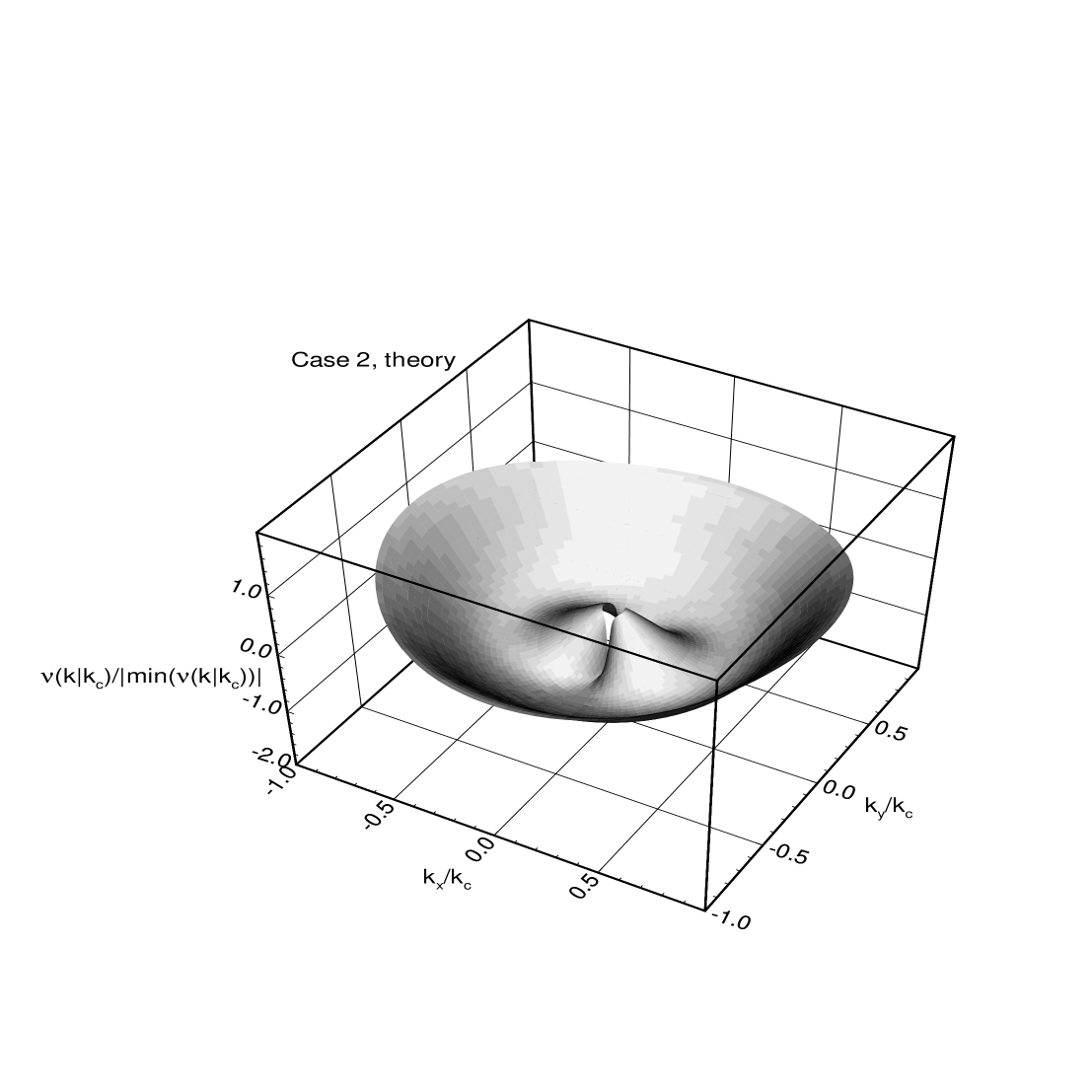
Figure 9: RG-derived two-parametric viscosity normalized by the absolute value of its minimum for $\beta$-plane turbulence. Parameter setting corresponds to Case 2 DNS.

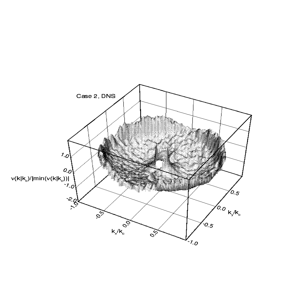
Figure 10: DNS-based two-parametric viscosity normalized by the absolute value of its minimum for Case 2 of $\beta$-plane turbulence.

This two-parametric viscosity was calculated analytically using the renormalization group (RG) theory of turbulence [25]; it is shown in Fig. 9 for the set of parameters corresponding to Case 2 of DNS. The behavior of the theoretically derived $\nu({\bf k}|k_{c})$ is quite similar to that obtained from DNS as shown in Fig. 10 also for Case 2. For large $k$, the $\beta$-effect is weak, and $\nu({\bf k}|k_{c})$ behaves similarly to the isotropic case [25, 12]; there is a sharp positive cusp and then $\nu({\bf k}|k_{c})$ becomes negative. As $k\to 0$, the effect of the $\beta$-term becomes stronger; $\nu({\bf k}|k_{c})$ remains negative in the vicinity of $\phi=\pm\pi/2$ but increases to zero in other directions. The negativity of $\nu({\bf k}|k_{c})$ along $\phi=\pm\pi/2$ is consistent with the strong energy flux into zonal jets as discussed in the previous section. It is important to mention that when the DNS integration was terminated, the low wavenumber end of the spectrum was not yet fully energy saturated. This fact explains the sharp increase in DNS-derived $\nu({\bf k}|k_{c})$ at small ${\bf k}$ evident in Fig. 10. The sign-changing structure of $\nu({\bf k}|k_{c})$ is indicative of a physical space SGS representation which combines a negative Laplacian and a positive (dissipative) hyperviscosity thus presenting an anisotropic version of the Kuramoto–Sivashinsky equation or SNV SGS representation [4]. The main ideas of the SNV formulation are discussed in the next section as applied to LES of more simple isotropic 2D turbulence. The isotropic SNV SGS representation can be useful for LES of $\beta$-plane turbulence with $k_{\beta}<k_{c}$ since deviation from isotropy is expected only for $k<k_{\beta}$ where, due to the factor of $k^{2}$ on the right hand side of (10) below, the SGS contribution is small.

4 SNV SGS Representation for Isotropic 2D Turbulence

Specific difficulties of LES of 2D turbulence in the energy transfer subrange are that the SGS representation must simultaneously be consistent with the conservation laws for both energy and enstrophy (or potential enstrophy) [4]. In addition, in LES of the inverse energy cascade, the wavenumber modes of the energy source lie in the subgrid scales so that the SGS representation must assume the function of the forcing. The SGS schemes being used to date in both 3D and quasi-2D flows usually employ Laplacian or higher order hyperviscosities that ensure SGS energy dissipation but not forcing. While such SGS are consistent with the dynamics of 3D turbulence where energy is directly cascaded from large to small scales where it dissipates, they cannot be expected to work well in quasi-2D flows where energy cascades from small to large scales while the enstrophy is transferred in the opposite direction. A possible resolution to this problem can involve the replacement of the SGS forcing by force located in the explicitly resolved region near $k_{c}$. However, this solution is not only quite cumbersome but also significantly distorts the explicit scales near $k_{c}$. In addition, this approach is difficult for implementation in physical space, particularly for bounded systems and/or systems with spatially nonuniform energy sources.

An alternative approach is offered by the SNV representation developed in [4] for isotropic 2D turbulence. In this approach, Eq. (1) (with $\beta$ = 0) that includes small scale forcing $\xi$ is replaced by LES equation

$${\partial\zeta({\bf k})\over\partial t} +\int_{|p|,|k-p|<{k_{c}}}{{\bf p}\times{\bf k}\over{p^{2}}}\zeta({\bf p})\zeta({\bf k}-{\bf p}){d{\bf p}\over{(2\pi)^{2}}}=-\nu(k|k_{c})k^{2}\zeta({\bf k}),$$

$$0<k<k_{c}.$$

Here, eddy viscosity is identified with the two-parametric viscosity $\nu(k|k_{c})$ defined by (9) (where, due to isotropy of the flow, the angular dependence is omitted). In [4] it was found that this eddy viscosity is given by

$$\nu(k|k_{c})={\epsilon\over 0.8\Omega(t)}N(k/k_{c}),$$ (11)

where $\Omega(t)$ is the total enstrophy of the system and $N(k/k_{c})\equiv\nu(k|k_{c})/|\nu(0|k_{c})|$ is plotted in Fig. 11. This formulation is designed to provide constant energy transfer with the rate $\epsilon$. Consistent with the eddy viscosity approach, the SGS representation (11) is a function of the flow. In a statistical steady state, Eq. (11) coincides with the two-parametric viscosity derived from the RG theory [4].

In a series of LES that employ the formulation (11) together with a specially designed large scale drag that effectively removes energy that reaches the largest computational scales, it was found that simulations can be carried out nearly indefinitely (being terminated after about 200 turnover times), while a very robust Kolmogorov $k^{-5/3}$ energy spectrum was established.

The formulation (11) can be simplified to make it more easily adaptable for simulations of quasi-2D flows in physical space. First, a two-term power series expansion in powers of $k/k_{c}$ that satisfies all necessary conservation laws can be derived from (11) [4],

$$\nu(k|k_{c})={25\over 18}{\epsilon\over\Omega(t)}\left[-1+{8\over 5}\left({k\over k_{c}}\right)^{2}\right].$$ (12)

Here, the negative term in the square brackets accounts for the effect of the small scale forcing and inverse energy cascade. The second term describes dissipative processes and is equivalent to a biharmonic viscosity in physical space. Then, (12) can be further simplified if $\Omega$ in its dissipative term is replaced by the value obtained from the Kolmogorov spectrum (4). Finally, the resulting SGS representation for 2D turbulence in the energy transfer subrange takes the form

$$\nu(k|k_{c})=-{25\over 18}{\epsilon\over\Omega(t)}+0.511\epsilon^{1/3}k_{c}^{-10/3}k^{2}.$$ (13)

In Figs 12 and 13, we plot the results of LES of 2D turbulence with the SGS representation (13). One can see that the total energy and enstrophy oscillate slightly around their steady state values while a robust Kolmogorov energy spectrum is established.

The corresponding physical space representation of the SGS operator for quasi-2D flows in the energy subrange is obtained using the inverse Fourier transform of (13),

$$-{\partial\over\partial x_{i}}\left(A_{2}{\partial\over\partial x_{i}}\right)-A_{4}{\partial^{4}\over\partial x_{i}^{2}\partial x_{j}^{2}},$$ (14)

where

$$A_{2} ={25\over 18}~{}{\epsilon\over\Omega({\bf x})},$$ (15)

$$A_{4} =0.511\epsilon^{1/3}(\Delta/2\pi)^{10/3},$$ (16)

and where $\Omega({\bf x})$ denotes the enstrophy averaged over an area adjacent to the grid cell, $\Delta$ is the grid resolution, the Laplacian term in (14) is written in the conservative form. Since (14) includes two terms, a negative Laplacian and positive (in the sense of dissipation) biharmonic, it is referred to as a stabilized negative viscosity (SNV) formulation. Generally, SNV equations are far more complicated than equations of the Kuramoto–Sivashinsky type [26, 27] because in the former, the coefficients are not constant but, as in the classical eddy viscosity approach, are functions of the flow.

5 Conclusions

In this paper, we describe results of direct numerical simulations of $\beta$-plane turbulence forced at small scales. As for isotropic 2D turbulence, nonlinear interactions play a crucial role in the evolution and dynamics of $\beta$-plane turbulence on all scales and at all times. The effect of the small scale forcing propagates to ever larger scales due to the inverse energy cascade. On relatively small scales, $k>k_{\beta}$, the flow is nearly isotropic and behaves like classical 2D turbulence. For modes with eddy turnover times comparable with the Rossby wave period, the turbulence energy spectrum begins to develop anisotropy that increases for $k\to 0$. It is found that for almost all $\phi$ except for the small vicinity of $\phi=\pm\pi/2$, the spectrum of turbulence is Kolmogorov-like, $E(k)\sim k^{-5/3}$. Around $\phi=\pm\pi/2$, or $|k_{x}|\to 0$, the two-parametric energy transfer function $\mathchar 29268\relax_{E}({\bf k}|k_{c})$ attains a sharp maximum, which indicates that there is a strongly anisotropic energy transfer into quasi-one-dimensional (zonal) structures. These zonal flows are generated and sustained by nonlinear processes, particularly, anisotropic inverse energy cascade. For $\phi\to\pm\pi/2$, the energy spectrum becomes very steep, $E(k)\sim k^{-5}$, as was first suggested by Rhines [6]. The steepening of the spectrum slows down flow evolution, to the extent that DNS even with relatively moderate resolution becomes computationally prohibitive. This difficulty can be resolved through LES of $\beta$-plane turbulence. For such LES, an SGS representation has been designed based upon a two-parametric viscosity. We have applied this approach for an example of isotropic 2D turbulence for which case the SGS representation is given by the SNV parameterization.

A.C. acknowledges fruitful discussions with V. Yakhot. This work has been supported by ARPA/ONR under Contract N00014-92-J-1796, ONR under Contract N00014-92-J-1363, NASA under Contract NASS-32804, and the Perlstone Center for Aeronautical Engineering Studies. The computations were performed on Cray Y-MP of NAVOCEANO Supercomputer Center, Stennis Space Center, Mississippi.

Figure 2: Energy spectra for $\phi=0$ (dotted line) and $\phi=\pi/2$ (dashed line) averaged in time and over a small surrounding sector $\pm\pi/12$ for $t/\tau_{tu}$ = 0.63, 1.19, and 8.32 for $\beta$ = 0 (Case 1) (due to the central symmetry, only these two directions are shown). Long dashed lines depict slopes of $-5$ and $-5/3$.

Figure 3: Same as in Fig. 2 but for $t/\tau_{tu}$ = 0.63, 1.19, and 16.25 and $\beta$=0.053 (Case 2).

Figure 4: Same as in Fig. 2 but for $t/\tau_{tu}$ = 0.63, 1.19, and 30.12 and $\beta$=0.3 (Case 3).

Figure 5: Compensated energy spectrum for Cases 2 (dashed line) and 3 (solid line) for $t/\tau_{tu}$ = 16.25 and 30.12, respectively.

Figure 7: Instantaneous vorticity field $\zeta({\bf x},t)$ at $t/\tau_{tu}=39.6$. (Too big for this archive, available upon request.)

Figure 8: Zonally-averaged velocity profile $U(y,t)$ (left column) and its second derivative $U_{yy}(y,t)$ (right column) for Case 3 at (from top to bottom) $t/\tau_{tu}$= 21.8, 39.6, and 59.4.

Figure 11: Function $N(k/k_{c})$ obtained from DNS (dots), TFM (dashed line) and RG (solid line) (from [12]).

Figure 12: Evolution of the total energy $E(t)$ (a) and enstrophy $\Omega(t)$ (b) in LES of isotropic 2D turbulence. In (a) we also plot the evolution of $E(t)$ with the energy of the 4th, 5th, 6th and 7th modes removed.

Figure 13: Time averaged energy spectrum for LES of isotropic 2D turbulence. The solid line depicts the Kolmogorov $-5/3$ slope.

References

- [1] J. Pedlosky, Geophysical Fluid Dynamics (Second Edition. Springer-Verlag, Inc., 1987).
- [2] R. Kraichnan, Inertial ranges in two-dimensional turbulence, Phys. Fluids 10 (1967) 1417–1423.
- [3] R. Kraichnan, Inertial-range transfer in two- and three-dimensional turbulence, J. Fluid Mech. 47 (1971) 525–535.
- [4] S. Sukoriansky, A. Chekhlov, B. Galperin, and S. Orszag, Large eddy simulation of isotropic two-dimensional turbulence in the energy subrange, J. Sci. Comput. (1995) in press.
- [5] R. Kraichnan and D. Montgomery, Two-dimensional turbulence, Rep. Prog. Phys. 43 (1980) 547–619.
- [6] P. Rhines, Waves and turbulence on a -plane, J. Fluid Mech. 69 (1975) 417–443.
- [7] G. Vallis and M. Maltrud, Generation of mean flows and jets on beta plane and over topography, J. Phys. Oceanogr. 23 (1993) 1346–1362.
- [8] G. Holloway, Contrary roles of planetary wave propagation in atmospheric predictability, in: G. Holloway and B.J. West, eds., Predictability of Fluid Motions (American Institute of Physics, New York, 1984) 593–599.
- [9] G. Holloway, Eddies, waves, circulation, and mixing: Statistical geofluid mechanics, Ann. Rev. Fluid Mech. 18 (1986) 91–147.
- [10] R. Panetta, Zonal jets in wide baroclinically unstable regions: persistence and scale selection, J. Atmos. Sci. 50 (1993) 2073–2106.
- [11] J. Whitaker and A. Barcilon, Low-frequency variability and wavenumber selection in models with zonally symmetric forcing, J. Atmos. Sci. 52 (1995) 491–503.
- [12] A. Chekhlov, S. A. Orszag, S. Sukoriansky, B. Galperin and I. Staroselsky, Direct numerical simulation tests of eddy viscosity in two dimensions, Phys. Fluids 6 (1994) 2548–2550.
- [13] L. Smith and V. Yakhot, Bose condensation and small-scale structure generation in a random force driven 2D turbulence, Phys. Rev. Lett. 71 (1993) 352–355.
- [14] L. Smith and V. Yakhot, Fine-size effects in forced two-dimensional turbulence, J. Fluid Mech. 274 (1994) 115–138.
- [15] G. Holloway and M. Hendershott, Stochastic closure for nonlinear Rossby waves, J. Fluid Mech. 82 (1977) 747–765.
- [16] R. Kraichnan, Eddy viscosity in two and three dimensions, J. Atmos. Sci. 33 (1976) 1521–1536.
- [17] R. Dickinson, Development of a Rossby wave critical level, J. Atmos. Sci. 27 (1970) 627–633.
- [18] J. Geisler and R. Dickinson, Numerical study of an interacting Rossby wave and barotropic zonal flow near a critical level, J. Atmos. Sci. 31 (1974) 946–955.
- [19] P. Haynes, The effect of barotropic instability on the nonlinear evolution of a Rossby wave critical layer, J. Fluid Mech. 207 (1989) 231–266.
- [20] P. Haynes, and M. McIntyre, On the representation of Rossby wave critical layers and wave breaking in zonally truncated models, J. Atmos. Sci. 44 (1987) 2359–2382.
- [21] P. Killworth and M. McIntyre, Do Rossby wave critical layers absorb, reflect, or over-reflect? J. Fluid Mech. 161 (1985) 449–492.
- [22] M. Lesieur, Turbulence in Fluids (Second Revised Edition. Kluwer Academic Publishers, 1990).
- [23] M. Longuet-Higgins and A. Gill, Resonant interactions between planetary waves, Proc. Roy. Soc. A299 (1967) 120–140.
- [24] A. Newell, Rossby wave packet interactions, J. Fluid Mech. 35 (1969) 255–271.
- [25] S. Sukoriansky, B. Galperin, and I. Staroselsky, Large-scale dynamics of two-dimensional turbulence with Rossby waves, in: H. Branover and Y. Unger, eds., Progress in Turbulence Research 162, (American Institute of Astronautics and Aeronautics, Washington, DC) 108–120.
- [26] S. Gama, U. Frisch, and H. Scholl, The two-dimensional Navier-Stokes equations with a large-scale instability of the Kuramoto-Sivashinsky type: Numerical exploration on the connection machine, J. Sci. Comput. 6 (1991) 425–452.
- [27] S. Gama, M. Vergassola, and U. Frisch, Negative eddy viscosity in isotropically forced two-dimensional flow: linear and nonlinear dynamics, J. Fluid Mech. 260 (1994) 95–125.