Statistical Test for Dynamical Nonstationarity in Observed Time-Series Data

Abstract

Information in the time distribution of points in a state space reconstructed from observed data yields a test for “nonstationarity”. Framed in terms of a statistical hypothesis test, this numerical algorithm can discern whether some underlying slow changes in parameters have taken place. The method examines a fundamental object in nonlinear dynamics, the geometry of orbits in state space, with corrections to overcome difficulties in real dynamical data which cause naive statistics to fail.

Since the discovery of the time-delay embedding for state-space reconstruction[1, 2, 3] a significant effort has been devoted to the development of techniques to extract information in observed time-series data from a geometrical, dynamical viewpoint. Underlying nearly all of these techniques ([4] is a review) is an assumption of stationarity: the dynamical process, and hence the geometrical attractor containing the orbits, has not changed on long time scales the order of the length of the dataset. If not true, there may be significant behavior on timescales longer than may be reliably resolved with the given data, or perhaps, experimental parameters, presumed fixed, have actually changed during the run.

Despite its nearly universal assumption, there is little previous literature on reliably testing for stationarity in physical situations. This work demonstrates a statistic and associated hypothesis test which sensitively detects nonstationary behavior given broadband and potentially chaotic data. A stationary dataset is presumed to to be sufficiently long to trace out a good approximation to the invariant measure. The algorithm described in this work quantifies “how much has the invariant measure, as inferred from the observations, changed over long timescales” and whether “this change is statistically significant.”

One could imagine measuring any number of simple statistics, such as the mean or standard deviation, from the two halves of the time series, and constructing a hypothesis test based on their presumed equality, but such techniques are not particularly good. First, the statistic is arbitrary and not related to the natural geometrical properties of the attractor, which we presume is the interesting object when analyzing chaos and other dynamical data. If not the mean or first moment, one could have chosen the average of, say, the third Legendre polynomial of the orbit point dotted into some arbitrary vector, et cetera, until one found the answer one wanted. Unless the particular statistic estimates a parameter deemed physically or dynamically important, such arbitrary choices are not particularly enlightening, and their power against various sorts of nonstationarity vary greatly. Second, naively applying procedures greatly overestimates the significance of differences: observed dynamical data are far from uncorrelated yet the simple, classical statistical estimations of confidence rely on the notion of independent observations. For example, measuring empirical means of first and second halves of a chaotic dataset and performing the classical $t$-test for their equality will quite often spuriously (and vehemently) reject the null hypothesis of stationarity, even when the data come from clean stationary experiments or well-known simple models such as the Lorenz attractor. Such methods do not not reliably diagnose the intuitive concept of dynamical stationarity that a typical physicist would imagine.

The present work attempts to rectify these two issues. One, by measuring a quantity related to geometrical properties in the full state space, and two, by accounting for the temporal dependence intrinsic in orbits from a continuous-time dynamical system. Furthermore, the method does not require artificially partitioning the time series into halves or other smaller time segments.

I sidestep direct estimations of the invariant measure from observed data. Counting points in boxes of state space, as used for computing mutual information [6], for instance, introduces potentially problematic issues such as the arbitrary choice of box size, quantization artifacts, and poor scaling with the embedding dimension. Kernel density estimators are computationally intensive in higher dimensions and functionals or statistics on such estimates may require difficult multi-dimensional integrals. The formalism does not naturally offer clear tests for significance.

Instead, the solution adopted quantifies nonstationarity using properties of nearest neighbors in state space. Neighbor searching is efficient and the estimates of consequent properties do not have a prima facie exponential “curse of dimensionality”. Neighbor statistics were used in [7, 8] to determine minimum embedding dimension for reconstruction, and to quantify predictability of observed chaotic data [5].

As background motivation, suppose we have two empirical probability distributions $\rho_{1}$ and $\rho_{2}$, the measures in the first and second halves of the dataset. One wonders whether $\rho_{1}=\rho_{2}$. Rewrite as

$$\rho_{1} = \frac{\rho_{1}+\rho_{2}}{2}+\frac{\rho_{1}-\rho_{2}}{2}=\rho_{0}+\delta\rho$$ (1)

$$\rho_{2} = \frac{\rho_{1}+\rho_{2}}{2}-\frac{\rho_{1}-\rho_{2}}{2}=\rho_{0}-\delta\rho$$ (2)

Given some x from the first half consider the probability that its nearest neighbor $\mbox{\bf x}^{nn}$ is also in the same half. Assuming $\rho(\mbox{\bf x}^{nn})\approx\rho(\mbox{\bf x})$, $p_{\mbox{same}}=\frac{\rho_{1}}{\rho_{1}+\rho_{2}}=\frac{\rho_{0}+\delta\rho}{2\rho_{0}}$. The expected proportion of matches is thus

$$\int d\mbox{\bf x}\rho_{1}(\mbox{\bf x})p_{\mbox{same}}=\langle\frac{(\rho_{0}+\delta\rho)^{2}}{2\rho_{0}}\rangle_{\mbox{first half}}.$$

With the same argument for the second half we find the overall expectation of seeing same-half matches is

$$E(\mbox{same}) = \langle\frac{(\rho_{0}-\delta\rho)^{2}+(\rho_{0}-\delta\rho)^{2}}{2\rho_{0}}\rangle$$ (3)

$$= \langle\frac{\rho_{0}^{2}+\delta\rho^{2}}{2\rho_{0}}\rangle=\frac{1}{2}+\langle\frac{\delta\rho^{2}}{2\rho_{0}}\rangle.$$ (4)

Nonstationarity, i.e. $\delta\rho\neq 0$, always increases this quantity, meaning that neighbors in state space are especially close in time when the distribution drifts over time.

The actual statistic feels the same effect but is more subtle: one collects the distribution of $D\equiv|\Delta(\mbox{\bf x})|\equiv|(T(\mbox{\bf x}^{nn})-T(\mbox{\bf x})|$ for all observed x, where $T(\cdot)$ denotes the time index of the point. Nonstationarity induces an excess number of small values of $D$ than otherwise expected.

Naively counting up the $D$ from all points and their nearest neighbors does not render a successful algorithm. As with computing the correlation dimension [9], one must exclude neighbors close in time because they are not independent of the reference point. If a prospective neighbor would result in $D=|T(\mbox{\bf x}^{nn})-T(\mbox{\bf x})|<W$, ignore it and continue searching instead. The interval $W$ is set to a characteristic autocorrelation time, perhaps 3 to 5 times the first minimum of mutual information.

Equally important, but less obvious, is accounting for serial correlation of neighboring trajectories: iterates of nearest neighbors often remain nearest neighbors, but this does not give new information. The present algorithm gathers multiple pairs of points and their neighbors which share the same $\Delta$ into the same strand. If the $\Delta$ associated with $\mbox{\bf x}(i)$ is the same as that for $\mbox{\bf x}(i-k)$ for any $k\in[1,W]$ append $\mbox{\bf x}(i)$ and its nearest neighbor to the strand associated with $\mbox{\bf x}(i-k)$. Otherwise, start a new strand with $\mbox{\bf x}(i)$ and its nearest neighbor with the as yet sole element. Note that elements of a single strand are not necessarily consecutive; there can be a gap up to $W$ timesteps long, though this is rarely realized in practice. Allowing such gaps prevents noise from damaging the proper accounting of neighbor correlations. Strands have two pieces, the “reference” section and the “neighbor” section, whose underlying points are nearest neighbors to the points in the reference section.

The final correction culls strands which share underlying points, whether in the reference or neighbor part, because their information is not completely independent. If any pair of strands share any points, we randomly delete one of the strands until no remaining strands share any points. Without the corrections, the “N” used in statistics is larger than it should be and would cause spurious null violations.

We test the observed distribution of $D$ for the final set of strands against the distribution expected under the null hypothesis of stationarity. The null assumes the time index of a neighbor is independent from that of the reference. For each observed strand, we pretend that the neighboring portion could have started at any time index in $[1,N]$ with equal probability, excluding the interval $W$ steps before the start and $W$ steps after the end of the reference portion. This generates an expected distribution of $D$ focused around that one strand; we repeat for all strands, generating the overall expected distribution of $D$, and normalize when done. This procedure takes computation time $O(N_{\mbox{points}}\cdot N_{\mbox{strands}})$ and so may be slow. An approximation good for reasonably large $N$ is the triangular shaped function derived by considering strands as points:

$$p(D)$$

with $M$ chosen to normalize $p(D)$. Figure 1 shows an example observed and expected distribution as an illustration of the typical shape.

This picture suggests using the Kolmogorov-Smirnov test on observed and expected $p(D)$. In practice, that statistic turned out overly sensitive to medium time-scale dynamical fluctuations observed even in stationary attractors. Instead, a “sign test” provides an even simpler and effective test which is most sensitive to the long timescale changes characteristic of nonstationarity. Denote the location at the median of the expected distribution as $D^{*}$. Then one counts the proportion of actually observed strands with $D<D^{*}$, $p=N_{\mbox{observed}}/N_{\mbox{strands}}$. One expects $p_{0}=0.5$. Under the null hypothesis,

$$z=\left(p-p_{0}\right)\left({N_{\mbox{strands}}}^{-1}p_{0}(1-p_{0})\right)^{-1/2}$$ (5)

is $N(0,1)$. Thus if one observes $z>2.36$ one rejects the null at the 99% confidence level. Unlike a K-S test, this sign test ensures that the violation be in the proper direction to be caused by nonstationarity, which causes large values of $p$ and hence $z$. Significant, but negative values of $z$ suggest important non-uniform neighbor time differences distinct from nonstationarity. Strong low-frequency periodic behavior seems able to produce such results.

Any statistical inference is only as good as its assumptions, in this case, that all strands are completely independent, and that in stationary systems nearest neighbor time-delays are distributed completely uniformly. This is indeed true for unbiased stochastic draws from probability densities, but is only an approximation for real dynamical systems. In constrast to the simple assumptions of classical statistics the diversity of possible behaviors under nonlinearity makes it very difficult to construct any interesting test where chaos is the null, something surrogate data methods do not attempt. The present test does so by testing for one specific aspect of dynamical systems and making an approximation that empirically appears to reasonably good. The main problem is that the “level” of the test, the frequency of finding $z>2.36$ under stationary conditions, is not exactly calibrated to the supposed 1%. This does not seem to be resolvable in general unless one had large amounts of the specific attractor observed in stationary conditions which would generate the actual distribution of $z$ in (5) instead assuming the normality. If the data were truly drawn independently and randomly from probability functions $\rho_{1}$ and $\rho_{2}$, the approximation is exact. The value of this method is an approach and approximation that works for many sorts of realistic datasets without requiring a large database of previously observed stationary orbits.

A computationally expensive but valuable confirmation protocol is to examine the proportion of $z$ values which reject the null as computed using randomly selected contiguous subsegments of lengths $N^{*}<N$ of the original data: a “poor-man’s bootstrapping”. With authentically nonstationary behavior, this proportion rises steadily with $N^{*}$. One may also examine the behavior with $N^{*}$ of $p$ averaged over subsamples as well as its effective significance via (5) to check whether $p$ grows consistently large with $N^{*}$ and not just wider than $N(0,1)$.

Figure 2 demonstrates the importance of the strand corrections. The data come from an experimental nonlinear circuit used to investigate synchronization and chaotic communications. The dynamics are known to be low-dimensional and the data clean. In any useful sense the data are quite stationary, yet the uncorrected statistic shows large violations, as would naive tests found in statistical textbooks such as equality of means or variances tried on first and second halves. By constrast, the present method shows no spurious null violations above the expected proportion. Consistent with the bootstrapping analysis, the dataset in toto violates the null without strand corrections but is consistent when those corrections are reinstated.

The next example demonstrates a more concrete engineering application. The data set was the pressure drop across a 15cm gap in a “fluidized bed reactor”, consisting of glass particles 2.7mm mean diameter in a 10cm diameter vertical cyclinder with air blown at constant flow from the bottom, a small scale model of industrial chemical reactors. For some external parameter regimes, the mass of particles undegoes complex motion which appears to be a combination of low-dimensional bulk dynamics and small-scale high-dimensional turbulence of the individual particles.[10] The observed variable was a pressure difference between two vertically separated taps. Figure 3 shows portions of time-delay embedding of orbits sections of the dataset taken at the same experimental parameters, and one when the air flow was boosted by 5%. The change in the attractor is rather subtle and difficult to reliably diagnose by eye. The statistic distinguishes them easily: Figure 4 shows the bootstrapping result on three datasets, one under stationary conditions, and one with a step change to the higher flow, and one with a slow ramp to that same flow. The lower right figure (not the upper left) is from the data taken at a different flow rate than the others.

The author has applied the method to quite a variety of data sets, simulated and experimental, and it yields correct and appropriate results in all cases found so far. It is not sensitive to reconstruction parameters and does not require the data to be known a priori to be clean low-dimensionality: it is not clear whether the fluidized bed datasets analyzed herein are better described as “chaos” or “very noisy periodicity”.

There is a whole class of related statistics that use the same neighbor principle. Instead of $|(T(\mbox{\bf x}^{nn})-T(\mbox{\bf x})|$ one may use the distribution of any general function $f(\mbox{\bf x}^{nn},\mbox{\bf x})$. For instance, $f(\cdot,\cdot)$ may be the “indicator function”, yielding 1 if both its arguments come from the same dataset and 0 otherwise. This provides a test for equivalence of the two data sets and can also yield a distance measure. The author has already done so to implement a “change-point-detector” which accurately finds the particular moment in time when some underlying parameter had changed, and the statistical confidence of its authenticity. Choosing $f=|\sin(\Omega T(\mbox{\bf x}^{nn})+\Phi)-\sin(\Omega T(\mbox{\bf x})+\Phi)|$ yields a test for the presence, and statistical significance, of a slow periodic modulation of the underlying attractor. If one has measured some other slowly varying signal $y(t)$, then the choice of $f=|y(T(\mbox{\bf x}^{nn}))-y(T(\mbox{\bf x}))|$ provides a test whether there is any statistically significant dynamical correlation betwen $y$ and the pattern of orbits traced out by x. For instance, one might wish to test the hypothesis that somehigh-frequency weather patterns in x is significantly correlated with historical $CO_{2}$ levels. These variations, alternative stationarity algorithms based on the correlation integral, as well as more extensive experimental results will be investigated in the author’s forthcoming research.

Isliker and Kurths [11] propose testing the one dimensional marginal distribution of the data for stationarity, but this ignores dynamical time domain information, and their method does not appear to account for serial correlation. Brown et al[12] synchronize empirical ODE models to time series, and propose using a long term increase in deviation as a measure of nonstationarity. This method appears powerful and relies on non-trivial dynamical information but requires clean low-dimensional data and does not provide an obvious statistical test.

The author is indebted to many discussions with C. Stuart Daw, Charles Finney, Ke Nguyen, and Martin Casdagli. This research was supported by the Department of Energy Distinguished Postdoctoral Fellow program.

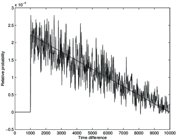
FIG. 1.: An example of expected and observed probability density functions for $D$ under the null hypothesis.

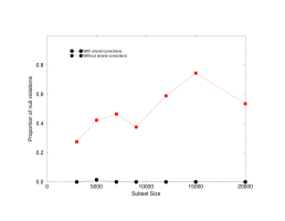
FIG. 2.: Proportion of rejections as a function of subsample size when strand corrections are turned off and on. Data set is from a stationary low-dimensional chaotic circuit, but without strand corrections there is frequent suprious rejection of the null.

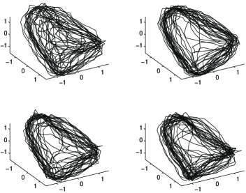
FIG. 3.: Phase space plots of the differential pressure signal from a fluidized bed reactor. Three are from the same parameters, one is different.

FIG. 4.: Proportion of rejections for stationary, step change and ramped air flow.

REFERENCES

- [1] Packard, N. H., J. P. Crutchfield, J. D. Farmer, and R. S. Shaw, 1980, Phys. Rev. Lett. 45, 712.
- [2] Takens, F., 1981, in Dynamical Systems and Turbulence, Warwick 1980, edited by D. Rand and L.-S. Young, Lecture Notes in Mathematics No. 898 (Springer, Berlin), p. 366.
- [3] Sauer, T., J. A. Yorke and M. Casdagli, “Embedology”, J. Stat. Phys. 65, 579-616 (1991).
- [4] Abarbanel, H. D. I., R. Brown, J. (“Sid”) Sidorowich, and Lev Sh. Tsimring, “The Analysis of Observed Chaotic Data in Physical Systems”, Reviews of Modern Physics 65, 1331-1392 (1993).
- [5] Casdagli, M. C., J. Roy. Stat. Soc. B 54, 303 (1991).
- [6] Fraser, A. M. and Swinney, H. L., “Independent Coordinates for Strange Attractors” Phys. Rev., 33A, 1134–1140 (1986).
- [7] Kennel, Matthew B., R. Brown, and Abarbanel, H. D. I. “Determining Minimum Embedding Dimension using a Geometrical Construction”, Phys. Rev. A 45, 3403-3411 (1992).
- [8] Kennel, Matthew B. and Abarbanel, H. D. I., “False Neighbors and False Strands: A Reliable Minimum Embedding Dimension Algorithm”, (1995), preprint available ftp://inls.ucsd.edu/pub/inls-ucsd/fns.tar.Z
- [9] Theiler, J. Phys. Lett. A 155 480-493 (1991).
- [10] Daw C. S. et al, Phys. Rev. Lett. 75 2308–2311 (1995).
- [11] Isliker, H. and J. Kurths Int. J. of Bif. and Chaos 3 1573–1579 (1993).
- [12] Brown, R., E. R. Rulkov, N. F. Tracy Phys. Rev. E 49 3784–3800 (1994).