Experimental studies of Chaos and Localization in Quantum Wavefunctions

Abstract

Wavefunctions in chaotic and disordered quantum billiards are studied experimentally using thin microwave cavities. The chaotic wavefunctions display universal density distributions and density auto-correlations in agreement with expressions derived from a 0-D nonlinear $\sigma$-model of supersymmetry, which coincides with Random Matrix Theory. In contrast, disordered wavefunctions show deviations from this universal behavior due to Anderson localization. A systematic behavior of the distribution function is studied as a function of the localization length, and can be understood in the framework of a 1-D version of the nonlinear $\sigma$-model.

Complexity in Quantum Mechanics can arise from two sources : chaos and disorder. Non-Integrable systems which are classically chaotic are now known to be of relevance to a variety of atomic and nuclear phenomena [1]. Disorder is of fundamental importance in condensed matter physics, where it leads to the phenomenon of localization [2]. For quantum chaotic systems, Random Matrix Theory (RMT) has been shown to provide a very good description of universal statistical properties of eigenvalue spectra [3, 4]. Recent developments in the theory of disordered systems based upon nonlinear $\sigma$-models using supersymmetry theory [5, 6, 7] have led to the recognition that the extreme diffusive limit of disordered systems also behave similarly to quantum chaotic systems. These theories have made several quantitative predictions for correlations in mesoscopic systems, including the contribution due to localization. However these ideas remain to be tested experimentally. Experiments also have added importance as several systems of Quantum Chaos which have localization, may behave similarly [8], for e.g. the kicked rotator, which has been studied numerically shows deviation from RMT behavior [9].

While the eigenvalue statistics of quantum chaotic systems has been experimentally tested, the eigenfunction statistics has not been done before. The principal reason is the lack of accessibility to wavefunctions. In atoms and nuclei, the nature of the wavefunctions only manifests indirectly in quantities such as transition rates. Experiments using microwave cavities which exploit the correspondence between the Maxwell and Schrödinger equations, are unique in that they allow direct measurement of the eigenfunctions, as well as eigenvalues, in model billiard geometries. Earlier such experiments have provided direct observation of scars [10], enabled precise tests of eigenvalue statistics[11], and have demonstrated ability to study arbitrary geometries which are not accessible to numerical simulation. In this paper we use such experiments to study the influence of chaos and localization on quantum wavefunctions.

The experiments were carried out using thin $(d<6$ mm$)$ cavities, whose cross-sections can be shaped in essentially arbitrary geometries. For these two dimensional cavities, the operational wave equation is $(\nabla^{2}\,+\,k^{2})\Psi=0$. The details of the experimental method are described in ref. [12]. Eigenfunctions were directly measured using a cavity perturbation technique which measures $|\Psi|^{2}$ [10, 12]. We study the manifestations of chaos and localization in terms of statistical properties of the eigenfunctions, such as the density probability distribution $P(|{\Psi}|^{2})$ and the density auto-correlation $P_{2}(r)=\ <|{\Psi(\stackrel{{\scriptstyle\rightarrow}}{{q}})}|^{2}|{\Psi(\stackrel{{\scriptstyle\rightarrow}}{{r}}+\stackrel{{\scriptstyle\rightarrow}}{{q}})}|^{2}>$, and the Inverse Participation Ratio (IPR), $P_{2}(r\rightarrow 0)$.

The geometries studied were representative of integrable, chaotic and disordered systems. Among chaotic systems, besides the quarter Sinai billiard, we also study the Sinai-Stadium geometry introduced by us in ref. [11]. The Sinai-Stadium has isolated periodic orbits (PO), and gives direct and exact agreement with RMT for the eigenvalue statistics, unlike the Sinai billiard and the stadium billiard for which the nonisolated PO contribution leads to deviations from universality [11]. Representative eigenfunctions for some of the geometries are shown in Fig.1. The 5.685 GHz (Fig. 1, top left) state of the Sinai-Stadium is similar to over almost a hundred other states of different energies that were observed, in that there are no visible scars that can be evidently associated with a PO. Indeed scarred states are few and the 7.370 GHz state shown in Fig. 1 (top right) is a rare coincidence with a whispering gallery PO.

Localization effects were observed by fabricating billiards in which tiles were placed to act as hard scatterers. These geometries are obtained by placing 1cm square or circular tiles in a 44 cm x 21.8 cm rectangle at random locations (Fig. 1). (The locations were generated using a random number generator and the tiles placed manually). Earlier experiments [13] on the eigenvalue spectrum of similar disordered geometries had shown that these experiments exemplify textbook two dimensional electron systems without interactions to remarkable degree. To our knowledge, these geometries are difficult to study using numerical computation and hence the microwave experiments at present afford the only reliable means to study this type of disordered systems. More than one realization of the disordered geometry was experimentally studied, labeled D1 through D5 depending on the density of scatterers (Table 1).

Sample eigenfunctions of D3, are shown in Fig. 1. Here again we have obtained nearly 100 wavefunctions. It is evident that in these billiards, any association with classical structures such as periodic orbits is difficult to see, although of course these billiards are also chaotic and such association must exist in principle. Instead the most striking effect visible is localization, which is strongest in the 3.372 GHz state, but is also present in a weaker form in the 6.651 GHz state. The degree of localization can be varied either by changing the frequency window for a given geometry, or changing the density of tiles. Hence the mean free path $l$ and also the localization length $\xi$ could be manipulated, the latter over almost two orders of magnitude.

We first carry out an analysis of the chaotic wavefunctions. $P(|{\Psi}|^{2})$ is shown in Fig.2 for the chaotic geometries - the Sinai-Stadium and the Sinai billiard. These are compared with the well-known Porter Thomas (P-T) distribution obtained from RMT [14]:

$$P(|{\Psi}|^{2})=\frac{1}{\sqrt{2\pi|{\Psi}|^{2}}}\exp(-\frac{|{\Psi}|^{2}}{2})$$ (1)

The best agreement is shown by the Sinai-Stadium. The Sinai billiard displays slight deviations which we attribute to states influenced by bouncing ball orbits. In an integrable system, the probability distribution is often truncated, e.g. for a rectangle at $|{\Psi}|^{2}=4$, and is not universal. In contrast, the chaotic wavefunctions show a finite, although exponentially vanishing probability of finding large intensities, in exact agreement with the P-T distribution, thus confirming their universal nature. Numerical simulations of random superpositions of plane waves was also done following ref. [15] and also shows very good agreement with P-T [16].

The density correlation $P_{2}(r)$ was also determined from the wavefunctions, and is shown in Fig.3. The angular brackets denote averaging over space $\stackrel{{\scriptstyle\rightarrow}}{{q}}$ , over angles between $\stackrel{{\scriptstyle\rightarrow}}{{q}}$ and $\stackrel{{\scriptstyle\rightarrow}}{{r}}$ , and finally over several states. An important aspect of the present work is that our experimental results for the chaotic and weak disorder cavities (see later) are well fit by the functional form :

$$P_{2}(r)\;=1+c\,J_{0}^{2}(kr)$$ (2)

where $k$ is the wave number. When computed for individual states, the result for $P_{2}(r)$ still has the functional form of Eq.(2), although the $r\rightarrow 0$ value is slightly different. However when averaged over several states, the resultant $P_{2}(r)$ is a robust quantity determined by the geometry alone. We further emphasize that we have checked and confirmed that $P_{2}(r)$ is isotropic for the Sinai-Stadium. The asymptotic value of $P_{2}(r\rightarrow\infty)=1$ can be understood since $P_{2}(r\rightarrow\infty)\rightarrow<|{\Psi(\stackrel{{\scriptstyle\rightarrow}}{{q}})}|^{2}><|{\Psi(\stackrel{{\scriptstyle\rightarrow}}{{q}})}|^{2}>\rightarrow 1$ as the wavefunctions are completely decorrelated at larger distances.

The data for the Sinai-Stadium yield $c=2\pm 0.1$. The Sinai billiard yields $c=1.7\pm 0.1$. An understanding of this value of $c=2$ can be achieved by noting that in general, $P_{2}(r\rightarrow 0)=<|{\Psi(\stackrel{{\scriptstyle\rightarrow}}{{q}})}|^{4}>=1+c$. If $x=|{\Psi(\stackrel{{\scriptstyle\rightarrow}}{{q}})}|^{2}$, then $P_{2}(r\rightarrow 0)=\int_{0}^{\infty}x^{2}P(x)dx$. Hence from Eq. 1 we get $P_{2}(r\rightarrow 0)=3$. Thus the value of $c=2$ for the chaotic case are consistent with the P-T distribution in Fig.2.

The functional form in Eq.(2) with $c=2$ has been anticipated by Prigodin, et. al. [6, 17] based upon a 0-D $\sigma$-model of supersymmetry. This theory is expected to apply to disordered systems in the diffusive limit, where the wavelength $\lambda<<l$ (scattering length) $<<L$, the cavity size. Results derived from this theory were earlier seen to coincide with RMT [5]. Therefore it gives P-T distribution for the eigenfunction components as in RMT. But it also gives coordinate correlations not available from RMT alone [6, 17]. On the basis that for the diffusive limit, the randomization due to disorder of an infinite system is the same as that due to chaos at the boundary of a finite system, the results should apply to chaotic systems. Our experiments confirm both these predictions of the 0-D $\sigma$-model for $P(|{\Psi}|^{2})$ and $P_{2}(r)$ in the chaotic cavities.

We now turn to an analysis of the eigenfunctions of the “disordered” geometries. We have divided the obtained wavefunctions into two regimes,(a) $\lambda>l$, i.e. the wavelength is greater than the mean free path. Here one observes strongly localized regions (Fig.1, bottom left). (b) At higher frequencies, where $\lambda<l$, the disordered eigenfunctions have the expected feature of having maxima apparently randomly distributed over the available domain (Fig.1, bottom right). In the experimental window from 2 to 8 GHz (15 to 3.2 cm), D1 is in regime (b), D2, D3 and D4 go from regime (a) to (b), and D5 is in regime (a).

Fig.4 displays the density probability $P(|{\Psi}|^{2})$ for D3 and D4, in regime (b) for data in the 6.5 to 7.75 GHz range. The disordered data are clearly not in agreement with the P-T distribution, displaying consistent and significant deviations at the high intensity end which are well beyond experimental error. These correspond to localized regions present in the disordered wavefunctions, in which the peak intensity is large compared to the average intensity.

Recently, Mirlin and Fyodorov have been able to calculate the localization corrections in a quasi one dimensional wire using a 1-D nonlinear $\sigma$-model of supersymmetry [7]. They have been also able to extend it to the full two dimensional case of the cavity in the delocalized regime [18]. For incipient localization, the results can be expressed as corrections to the P-T distribution given by:

$$P(x)=\,f(x)\exp(-x/2)/\sqrt{2\pi x}\,\,$$ (3)

where $x=|{\Psi(\stackrel{{\scriptstyle\rightarrow}}{{q}})}|^{2}$ as before and $f(x)=1+d(1/4-x/2+x^{2}/12)$ for small $d$. Now d depends on localization length $\xi$ and the density of disorder $l/L$ through $d=L/(2\pi\xi)ln(L/l)$ for the two dimensional case [18]. This form is plotted in Fig. 3 for D3 and shows that the 1-D $\sigma$-model gives an accurate description of the localization effects seen in the experiment. From the fit to data for D1 to D4 in the 6.5 to 7.75 GHz range, $\xi/L$ are extracted and listed in Table 1.

$P_{2}(r)$ for D3 is shown in Fig.5 and is well described by the functional form Eq.2. The $c$ value obtained from a fit is given in Table 1. This is consistent, within experimental error, with the values obtained directly from the density distribution in Eq. 3, by using $IPR=\int_{0}^{\infty}x^{2}P(x)dx=1+c=3+d[L/(\xi\pi)]ln(L/l)$. This higher value is therefore due to the high intensity peaks observed in Fig.1 and the non-P-T distribution function in Fig.4 and depends on the localization length.

In the strong localization regime (a) the deviations are even greater as the effects due to localization is even more pronounced. For strong localization, like in D5, stronger deviations in $P(|{\Psi}|^{2})$ are seen which cannot be described by corrections to P-T form as in Eq. 3. However the data is described well by expressions for strong localization, for the wire case, in ref. [7]. The form, $P(x)=8/(L/\xi)^{2}\sqrt{(L/\xi)/2x}K_{1}(2\sqrt{2x/(L/\xi)})$ fits well and a $\xi/L$ value of 0.1 can be extracted for the data in the 3 to 6 GHz range, however some constants due to dimensionality considerations are expected to change. $P_{2}(r)$ also does not obey the expression Eq. 2, as is evident from Fig.5. Instead spatial correlations die out faster, perhaps exponentially. Although the experimental data are available, further theoretical work needs to be done to compare the data in the strong and intermediate localization regime.

An important perspective can be gained by examining the IPR for different eigenstates that were measured for both the chaotic and the D3 and D4 cavities, as shown in the inset to Fig.5. It is seen to fluctuate from one eigenstate to the other - such level to level variations are expected to have important characteristics [18] which will be analyzed in future work. However the IPR for the chaotic cavity are confined to a band around the limiting value of 3, with an average of 3.2. In contrast the IPR for the disordered cavity, show an increase towards the lower eigenstates, which tend towards the strong localization regime, showing the dependence of localization length on the frequency and the transition from regime (a) to (b). Of course deeper into the diffusion regime in which the localization length becomes effectively “infinite”, at large $f$ or small $\lambda$, these also tend to 3, the value for the chaotic case. The dashed line represents the functional form for the IPR deduced above from eq.(3), and which extends up to the regime $\lambda<l$, and which thus represents the small localization limit of the 1-D $\sigma$-model.

In conclusion, we have been able to study the role of chaos and disorder in organizing quantum wavefunctions by means of electromagnetic experiments. The results demonstrate universal properties of chaotic wavefunctions, which also correspond to disordered systems in the extreme diffusive limit. They also demonstrate deviations from universality due to localization. The results appear to be consistent with a proposed notion of a (weaker) universality class [8] for systems with localization, in which the statistical measures depend on one additional parameter - the localization length. The disordered billiards used here are the first experimental realization of such a system in which quantitative results have been obtained, and the dependence on the parameter $\xi/L$ has been quantitatively demonstrated, enabling tests of the nonlinear $\sigma$-model of supersymmetry theory, originally intended for mesoscopic systems. These results are of potential relevance to systems such as mesoscopic devices [19] and acoustic and electromagnetic waves [20].

We thank V.Prigodin, B.Simons, Y.Fyodorov and A.Mirlin for useful discussions and communicating results prior to publication. This work was supported by the ONR under Grant No. N00014-92-J-1666.

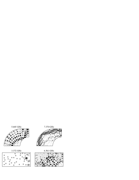
FIG. 1.: Representative eigenfunctions of the chaotic Sinai - Stadium billiard (top) and disordered geometry (bottom).

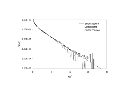
FIG. 2.: Density distribution $P(|{\Psi}|^{2})$ for the Sinai-Stadium and the Sinai billiard compared with the Porter-Thomas form from RMT. While the Sinai-Stadium is in excellent agreement, the Sinai Billiard data shows slight deviations due to states influenced by bouncing ball orbits.

FIG. 3.: Density correlation function $P_{2}(r)$ for the chaotic geometries. The solid line represents Eq.(2) with $c=2$ as expected from a supersymmetry approach.

FIG. 4.: $P(|{\Psi}|^{2})$ for two realizations of the disordered geometries, showing deviations from Porter-Thomas due to localization. The dashed line is a fit to Eq. 3. The dashed-dotted line is fit to the strong-localization form in the text.

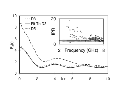
FIG. 5.: $P_{2}(r)$ for the disordered wavefunctions showing oscillations similar to the chaotic data. The solid line represents Eq.(2) with c = 3.5 and kr rescaled by 0.96. (Inset) The inverse participation ratio (IPR) vs. frequency for the D3 & D4 cavities (circles), and the chaotic cavity (squares). The dotted lines represent the limits of excursion of the chaotic data. The dashed curve represents the behavior expected on the basis of the 1-D $\sigma$ -model.

Cavity	No of scatterers	l, cm	L, cm	$\xi$/L	c
D1	12	9	32	10	2.85
D2	27	6	31	5	3.14
D3	36	5	31	4	3.50
D4	36	5	31	4	3.54
D5	72	3.5	30	-	-

TABLE I.: The various disordered cavities.

REFERENCES

- [1] M. Gutzwiller, Chaos in Classical and Quantum Mechanics (Springer-Verlag, New York, 1990).
- [2] P. W. Anderson, Phys. Rev. 109, 1492 (1958); E. Abrahams et al., Phys. Rev. Lett. 42, 673 (1979).
- [3] O. Bohigas, M. J. Giannoni, and C. Schmit, Phys. Rev. Lett. 52, 1 (1984).
- [4] M. L. Mehta, Random Matrices, 2nd ed. (Academic, New York, 1990).
- [5] K. B. Efetov, Adv. Phys. 32, 53 (1983).
- [6] V. N. Prigodin, B. L. Altshuler, K. B. Efetov, and S. Iida, Phys. Rev. Lett. 72, 546 (1994).
- [7] A. D. Mirlin and Y. V. Fyodorov, J. of Phys A: Math. Gen. 26, L551 (1993).
- [8] Y. Fyodorov, Phys. Rev. Lett., 73, 2688 (1994).
- [9] G. Casati et al., Phys. Rev. Lett., 64, 5 (1990).
- [10] S. Sridhar, Phys. Rev. Lett. 67, 785 (1991).
- [11] A. Kudrolli, S. Sridhar, A. Pandey, and R. Ramaswamy, Phys. Rev. E 49, R11 (1994).
- [12] S. Sridhar, D. Hogenboom, and B. A. Willemsen, J. Stat. Phys. 68, 239 (1992).
- [13] S. Sridhar et al., in Quantum Dynamics of Chaotic Systems (Gordon and Breach, Amsterdam, 1993), p. 297.
- [14] F. Haake, Quantum Signatures of Chaos (Springer-Verlag, Berlin, 1991).
- [15] P. O’Connor, J. Gehlen, and E. J. Heller, Phys. Rev. Lett. 58, 1296 (1987).
- [16] M. V. Berry, in Chaotic Behavior of Deterministic System (North Holland, New York, 1981), p. 171.
- [17] V. N. Prigodin, unpublished.
- [18] Y. Fyodorov and A. Mirlin, unpublished.
- [19] R. Jalabert et al., Phys. Rev. Lett. 65 2442 (1990);H. Baranger et al., Phys. Rev. Lett. 73, 142 (1994).
- [20] S. McCall, et al., Phys. Rev. Lett. 67, 2017 (1991).