Integrability and Ergodicity of Classical Billiards in a Magnetic Field

Abstract

We consider classical billiards in plane, connected, but not necessarily bounded domains. The charged billiard ball is immersed in a homogeneous, stationary magnetic field perpendicular to the plane.

The part of dynamics which is not trivially integrable can be described by a “bouncing map”. We compute a general expression for the Jacobian matrix of this map, which allows to determine stability and bifurcation values of specific periodic orbits. In some cases, the bouncing map is a twist map and admits a generating function. We give a general form for this function which is useful to do perturbative calculations and to classify periodic orbits.

We prove that billiards in convex domains with sufficiently smooth boundaries possess invariant tori corresponding to skipping trajectories. Moreover, in strong field we construct adiabatic invariants over exponentially large times. To some extent, these results remain true for a class of non-convex billiards.

On the other hand, we present evidence that the billiard in a square is ergodic for some large enough values of the magnetic field. A numerical study reveals that the scattering on two circles is essentially chaotic.

Key words: billiards, magnetic field, twist map, integrability,
adiabatic invariant, ergodicity

1 Introduction

We consider the classical motion of a particle of mass $m$ and charge $q$ in a plane domain $Q$. A homogeneous, stationary magnetic field $B$ perpendicular to the plane makes the particle move on arcs of Larmor radius $\mu$. Whenever it encounters the boundary, the particle is reflected specularly. This problem was first considered by Robnik and Berry ([RB], [Ro]).

One point of interest in such models is the problem of integrable versus ergodic behaviour of Hamiltonian systems. In zero field, we know examples of integrable billiards (elliptic or rectangular boundary) as well as ergodic ones (dispersive Sinai billiards, Bunimovich stadium, see for instance [KT]). Since it is unlikely that integrability is stable with respect to perturbation by a magnetic field, $B$ is a natural parameter for studying the transition from order to chaos. One question is whether the billiard can become globally ergodic in strong enough field.

Another motivation for studying magnetic billiards is connected to the problem of quantum chaos. Recently, it has become possible to create mesoscopic systems where the electrons’ motion is essentially ballistic [LRPW]. Behaviour of some macroscopic observables, like the susceptibility, can be surprisingly complicated [RKC], and may be related to classical dynamics. In order to be able to apply semi-classical methods like trace formulae, it is desirable to have a good knowledge of classical periodic orbits and their stability, at least perturbatively.

This paper is organized as follows. In section 2, we give a more precise definition of the billiard flow and boundaries considered. The interesting part of dynamics can be described by a bouncing map $T$, defined in section 3, where we also give an exact expression for the Jacobian matrix of $T$. In some cases, $T$ is a twist map and admits a generating function $G$. In section 4, we give an exact expression of $G$, and we discuss its physical interpretation and its practical applications.

Our main analytical results are contained in section 5, where we consider billiards with smooth, convex boundaries. Using perturbative techniques, we analyze different quasi-integrable limits. In section 5.2, we prove the existence of invariant curves for all values of the magnetic field. These quasi-periodic trajectories correspond physically to diamagnetic currents along the boundary. Our KAM type result generalizes the well known theorem of Lazutkin [L] on the existence of caustics near the boundary, in the zero field case. The magnetic field however breaks the symmetry between the forward and backward skipping orbits, and at intermediate values of the field, only one kind of skipping orbit is present. In section 5.3, we analyze the strong magnetic field limit. We compute an expansion of the bouncing map in powers of the Larmor radius and construct an adiabatic invariant on a time scale growing exponentially with the magnetic field when the boundary is analytic. At low order, this adiabatic invariant coincides with the one derived by Robnik and Berry. In order to construct the invariant, we derive a theorem on a class of maps of the annulus, which may be of interest in a broader context. Section 7 is devoted to the proof of it.

In section 6, we study billiards which may show an important chaotic component, because of singularities in the boundary (polygons) or because of a negative curvature. It turns out that the properties of billiards in convex domains can be to some extent generalized to billiards with concave boundary. In general it seems that billiards in a magnetic field are of the mixed type (invariant tori and chaotic components coexist). A possible exception is the case of the square at some particular values of the magnetic field, where we present an analytical argument and numerical evidence for a completely chaotic motion.

2 Definition of the billiards

Let $Q$ be a connected domain in ${\rm I\!R}^{2}$. We assume for simplicity that the boundary $\partial Q$ consists of simple, closed, piecewise $C^{2}$ curves of total length $\left|\partial Q\right|$, although some of our results may be extended to more general cases. Several of them however need a higher degree of differentiability, which will be clearly indicated on the spot.

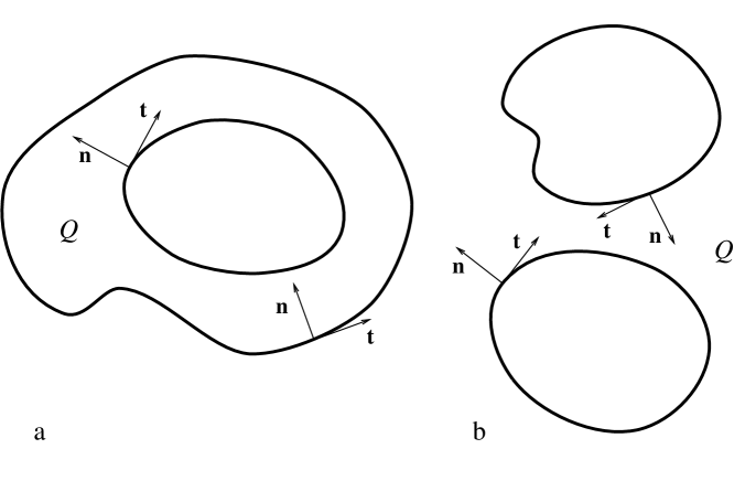
Figure 1: Examples of billiard domains $Q$, with tangent and normal vectors to the boundary $\partial Q$: (a) bounded domain, (b) unbounded domain.

The boundary is parameterized with the curvilinear abscissa or arclength $s$:

$$\mathchoice{\mbox{\boldmath$\displaystyle\bf x$}}{\mbox{\boldmath$\textstyle\bf x$}}{\mbox{\boldmath$\scriptstyle\bf x$}}{\mbox{\boldmath$\scriptscriptstyle\bf x$}}(s)=(X(s),Y(s)),\;\;ds^{2}=dX^{2}+dY^{2},\;\;s\in[0,\left|\partial Q\right|).$$ (1)

The unit tangent and normal vectors and the (signed) curvature are given by

$${\mbox{\boldmath$\bf t$}}(s) = (X^{\prime}(s),Y^{\prime}(s))=(\cos\tau(s),\sin\tau(s)),$$

$${\mbox{\boldmath$\bf n$}}(s) = (-Y^{\prime}(s),X^{\prime}(s)),$$

$$\kappa(s) = \frac{d\tau}{ds}=X^{\prime}(s)Y^{\prime\prime}(s)-X^{\prime\prime}(s)Y^{\prime}(s)=\frac{1}{\rho(s)}.$$ (2)

Parameterization is chosen in such a way that $\textstyle\bf n$ is always oriented towards the interior of $Q$ (see fig.1). In this way, the curvature is positive for a convex boundary. We suppose $\kappa(s)$ to be defined and continuous everywhere but on a set $E_{2}$ of punctual values of $s$. The vectors $\textstyle\bf t$ and $\textstyle\bf n$ are undefined on a set $E_{1}\subset E_{2}$.

Inside $Q$, the billiard flow is given by the Lagrangian

$$L(\mathchoice{\mbox{\boldmath$\displaystyle\bf x$}}{\mbox{\boldmath$\textstyle\bf x$}}{\mbox{\boldmath$\scriptstyle\bf x$}}{\mbox{\boldmath$\scriptscriptstyle\bf x$}},\dot{\mathchoice{\mbox{\boldmath$\displaystyle\bf x$}}{\mbox{\boldmath$\textstyle\bf x$}}{\mbox{\boldmath$\scriptstyle\bf x$}}{\mbox{\boldmath$\scriptscriptstyle\bf x$}}})=\frac{1}{2}m\mathchoice{\mbox{\boldmath$\displaystyle\bf\dot{x}$}}{\mbox{\boldmath$\textstyle\bf\dot{x}$}}{\mbox{\boldmath$\scriptstyle\bf\dot{x}$}}{\mbox{\boldmath$\scriptscriptstyle\bf\dot{x}$}}^{2}+q\left(\dot{\mathchoice{\mbox{\boldmath$\displaystyle\bf x$}}{\mbox{\boldmath$\textstyle\bf x$}}{\mbox{\boldmath$\scriptstyle\bf x$}}{\mbox{\boldmath$\scriptscriptstyle\bf x$}}}|\mathchoice{\mbox{\boldmath$\displaystyle\bf A$}}{\mbox{\boldmath$\textstyle\bf A$}}{\mbox{\boldmath$\scriptstyle\bf A$}}{\mbox{\boldmath$\scriptscriptstyle\bf A$}}(\mathchoice{\mbox{\boldmath$\displaystyle\bf x$}}{\mbox{\boldmath$\textstyle\bf x$}}{\mbox{\boldmath$\scriptstyle\bf x$}}{\mbox{\boldmath$\scriptscriptstyle\bf x$}})\right),\;\;\mathchoice{\mbox{\boldmath$\displaystyle\bf A$}}{\mbox{\boldmath$\textstyle\bf A$}}{\mbox{\boldmath$\scriptstyle\bf A$}}{\mbox{\boldmath$\scriptscriptstyle\bf A$}}(\mathchoice{\mbox{\boldmath$\displaystyle\bf x$}}{\mbox{\boldmath$\textstyle\bf x$}}{\mbox{\boldmath$\scriptstyle\bf x$}}{\mbox{\boldmath$\scriptscriptstyle\bf x$}})=(-\frac{1}{2}yB,\frac{1}{2}xB).$$ (3)

The resulting motion is simply circular uniform, with Larmor radius

$$\mu=\frac{mv}{\left|qB\right|}=\frac{\sqrt{2mE}}{\left|qB\right|},$$ (4)

where speed $v=\left|\dot{\mathchoice{\mbox{\boldmath$\displaystyle\bf x$}}{\mbox{\boldmath$\textstyle\bf x$}}{\mbox{\boldmath$\scriptstyle\bf x$}}{\mbox{\boldmath$\scriptscriptstyle\bf x$}}}\right|$ and energy $E$ are constants of motion. We adopt the sign convention $qB<0$, which implies that the particle turns counterclockwise, and we take some characteristic length of the billiard as a length unit, so that $\mu$ can be considered as a dimensionless parameter. Thus, increasing $B$ is equivalent to decreasing $E$ or increasing the size of the billiard (which can be viewed as taking the thermodynamic limit).

Each time the particle hits the boundary, the velocity changes according to the law of specular reflection $\mathchoice{\mbox{\boldmath$\displaystyle\bf v$}}{\mbox{\boldmath$\textstyle\bf v$}}{\mbox{\boldmath$\scriptstyle\bf v$}}{\mbox{\boldmath$\scriptscriptstyle\bf v$}}^{\prime}=\mathchoice{\mbox{\boldmath$\displaystyle\bf v$}}{\mbox{\boldmath$\textstyle\bf v$}}{\mbox{\boldmath$\scriptstyle\bf v$}}{\mbox{\boldmath$\scriptscriptstyle\bf v$}}-2\left(\mathchoice{\mbox{\boldmath$\displaystyle\bf v$}}{\mbox{\boldmath$\textstyle\bf v$}}{\mbox{\boldmath$\scriptstyle\bf v$}}{\mbox{\boldmath$\scriptscriptstyle\bf v$}}|\mathchoice{\mbox{\boldmath$\displaystyle\bf n$}}{\mbox{\boldmath$\textstyle\bf n$}}{\mbox{\boldmath$\scriptstyle\bf n$}}{\mbox{\boldmath$\scriptscriptstyle\bf n$}}\right)\mathchoice{\mbox{\boldmath$\displaystyle\bf n$}}{\mbox{\boldmath$\textstyle\bf n$}}{\mbox{\boldmath$\scriptstyle\bf n$}}{\mbox{\boldmath$\scriptscriptstyle\bf n$}}$, which is well defined for almost every point of the boundary.

The phase space $M=Q\times S^{1}$ can be divided into two disjoint sets $M_{1}$ and $M_{2}$. $M_{1}$ consists of all the orbits that never touch the boundary. It corresponds to an integrable component of the motion and may be empty. In non-zero magnetic field ($\mu<\infty$), the orbits of $M_{2}$ hit the boundary an infinite number of times. It is thus natural to study the dynamics in $M_{2}$ by means of a bouncing map.

3 The bouncing map and its Jacobian matrix

Let us consider the trajectory between two successive collisions with $\partial Q$, occurring at $P_{0}=(X(s_{0}),Y(s_{0}))$ and $P_{1}=(X(s_{1}),Y(s_{1}))$. The trajectory is an arc $\gamma$ of center $O$, radius $\mu$ and angle $\psi$ (see fig.2).

We call $\theta_{i}$ the angle between the arc and the boundary at $P_{i}$, and $u_{i}=-\cos{\theta_{i}}$, $i=0,1$. Quantities $s$ and $u$ are the Birkhoff variables and the bouncing map $T$ is defined as

$$T:(s_{0},u_{0})\mapsto(s_{1},u_{1}).$$ (5)

If $\ell$ is the length of the chord $P_{0}P_{1}$, and $\chi$ is the angle between the chord and the arc $\gamma$, simple geometry shows that

$$\psi=2\chi,\;\;\sin\chi=\frac{\ell}{2\mu}.$$ (6)

In general, there may be two trajectories with supplementary $\chi$ for a given $\ell$ (see also fig.13). This is a characteristic magnetic field effect.

Figure 2: The trajectory between two successive bounces is an arc $\gamma$ of radius $\mu$, angle $\psi$ and extremities $P_{0}$ and $P_{1}$. The Jacobian matrix of the bouncing map $T$ depends on the length $\ell$ of the chord, the angle $\chi$ between chord and arc, the angles $\theta_{0}$, $\theta_{1}$ between arc and boundary and the curvature at $P_{0}$, $P_{1}$.

Generalizing Birkhoff’s technique ([B], p.173, see also [KT]), we find

Proposition 1 If $s_{0},s_{1}\not\in E_{2}$, the Jacobian matrix $DT$ of $T$ is given by

$$\frac{\partial s_{1}}{\partial s_{0}} = \frac{\kappa_{0}\ell\cos\chi-\sin(\theta_{0}+2\chi)}{\sin\theta_{1}}$$

$$\frac{\partial s_{1}}{\partial u_{0}} = \frac{\ell\cos\chi}{\sin\theta_{1}\sin\theta_{0}}$$

$$\frac{\partial u_{1}}{\partial s_{0}} = \frac{\sin(\theta_{0}+2\chi)\sin(\theta_{1}+2\chi)-\sin\theta_{0}\sin\theta_{1}}{\ell\cos\chi}$$

$$-\kappa_{0}\sin(\theta_{1}+2\chi)-\kappa_{1}\sin(\theta_{0}+2\chi)+\kappa_{0}\kappa_{1}\ell\cos\chi$$

$$\frac{\partial u_{1}}{\partial u_{0}} = \frac{\kappa_{1}\ell\cos\chi-\sin(\theta_{1}+2\chi)}{\sin\theta_{0}}$$ (7)

where $\kappa_{i}=\kappa(s_{i})$.

For completeness and consistency of notation, we give a proof in appendix A. We noticed that an alternative proof of this formula was provided by [MBG]. All the quantities appearing in (3) can be easily expressed as functions of $s_{0}$ and $s_{1}$ (see (79) and (80)). It is in general much more difficult to solve the relation $u_{0}(s_{0},s_{1})$ with respect to $s_{1}$, in order to obtain $DT$ as a function of $z_{0}=(s_{0},u_{0})$.

A first observation is that $DT$ has unit determinant, and hence the Birkhoff variables are conjugate, although momentum and velocity are not collinear in a magnetic field (see section 4).

A second observation concerns the element $\frac{\partial s_{1}}{\partial u_{0}}$. We see that its sign depends only on $\chi$. Suppose that the shape of $Q$ is such that it cannot contain any arc of radius $\mu$ and angle larger than $\pi$. Then we have $\frac{\partial s_{1}}{\partial u_{0}}>0$, and $u_{0}$ is uniquely defined for given $s_{0}$ and $s_{1}$. In such a case, $T$ is called a (symplectic) twist map. Twist maps, especially when continuous, have a lot of properties (see e.g. [Me] for a review), some of which we will discuss in the next section.

The Jacobian matrix allows us to compute Liapunov exponents and to determine stability of periodic orbits. If we define for $z=(s,u)$ the stability matrix

$$S_{n}(z)=DT(T^{n-1}z)\cdots DT(Tz)DT(z),$$ (8)

then the Liapunov exponents are given by

$$\Lambda_{\pm}(z)=\pm\lim_{n\rightarrow\infty}\frac{1}{2n}\ln\mathchoice{\mbox{$\displaystyle\rm Tr$}}{\mbox{$\textstyle\rm Tr$}}{\mbox{$\scriptstyle\rm Tr$}}{\mbox{$\scriptscriptstyle\rm Tr$}}S_{n}^{\mathchoice{\mbox{$\displaystyle\rm T$}}{\mbox{$\textstyle\rm T$}}{\mbox{$\scriptstyle\rm T$}}{\mbox{$\scriptscriptstyle\rm T$}}}(z)S_{n}(z).$$ (9)

If $z$ belongs to an orbit of period $n$, the orbit is hyperbolic and unstable if $\left|\mathchoice{\mbox{$\displaystyle\rm Tr$}}{\mbox{$\textstyle\rm Tr$}}{\mbox{$\scriptstyle\rm Tr$}}{\mbox{$\scriptscriptstyle\rm Tr$}}S_{n}(z)\right|>2$, parabolic if $\left|\mathchoice{\mbox{$\displaystyle\rm Tr$}}{\mbox{$\textstyle\rm Tr$}}{\mbox{$\scriptstyle\rm Tr$}}{\mbox{$\scriptscriptstyle\rm Tr$}}S_{n}(z)\right|=2$ and elliptic if $\left|\mathchoice{\mbox{$\displaystyle\rm Tr$}}{\mbox{$\textstyle\rm Tr$}}{\mbox{$\scriptstyle\rm Tr$}}{\mbox{$\scriptscriptstyle\rm Tr$}}S_{n}(z)\right|<2$. In the latter case, the orbit is stable unless resonance occurs. In section 6, we will give examples of how to apply the formula (3) to analyze stability of specific families of periodic orbits.

4 Generating functions

Here we call generating function of the continuous map $T$ a $C^{1}$ function $G(s_{0},s_{1})$ such that

$$dG=u_{0}ds_{0}-u_{1}ds_{1}.$$ (10)

It is easy to check the following properties [Me]:

1. If $T$ is an area preserving twist map, it admits a generating function, unique up to an additive constant, given by

   $$G(s_{0},s_{1})=\int^{(s_{0},s_{1})}u_{0}(\xi,\eta)d\xi-u_{1}(\xi,\eta)d\eta.$$ (11)

2. If $G$ is $C^{2}$, the map $T$ generated by $G$ is always area preserving. It is a twist map if $\partial^{2}_{s_{0}s_{1}}G>0$ .

3. If $G$ is $C^{2}$, $u$ is a constant of motion iff $G(s_{0},s_{1})=g(s_{1}-s_{0})$.

In zero field, $G$ is known to be the length of the chord $\ell(s_{0},s_{1})$. For magnetic billiards, we found that $G$ depends also on an area associated to the trajectory, a feature appearing apparently in all problems involving a magnetic field:

Proposition 2 Suppose that $Q$ is bounded and that $T$ is a twist map. Then, for $s_{0},s_{1}\not\in E_{2}$, the generating function is given by

$$G={\cal L}+\frac{1}{\mu}{\cal S},$$ (12)

where ${\cal L}$ is the length of the arc and $\cal S$ is the area between the arc and the boundary (see fig.3).

We give the proof in appendix B. For practical purposes, it is useful to write $G$ in the form

$$G(s_{0},s_{1})=\frac{1}{\mu}A(s_{0},s_{1})+B_{\mu}(\ell(s_{0},s_{1})),$$ (13)

where $A$, the area between the chord and the boundary, does not depend on the magnetic field, and

$$B_{\mu}(\ell)=\mu\mathchoice{\mbox{$\displaystyle\rm Arcsin$}}{\mbox{$\textstyle\rm Arcsin$}}{\mbox{$\scriptstyle\rm Arcsin$}}{\mbox{$\scriptscriptstyle\rm Arcsin$}}\left(\frac{\ell}{2\mu}\right)+\frac{\ell}{2}\sqrt{1-\frac{\ell^{2}}{4\mu^{2}}}$$ (14)

is equal to ${\cal L}$ minus the area between the chord and the arc, divided by $\mu$.

As an example, let us consider an elliptic boundary, of equation

$$\mathchoice{\mbox{\boldmath$\displaystyle\bf x$}}{\mbox{\boldmath$\textstyle\bf x$}}{\mbox{\boldmath$\scriptstyle\bf x$}}{\mbox{\boldmath$\scriptscriptstyle\bf x$}}=(\lambda\cos\varphi,\sin\varphi),\;\;\;\frac{ds}{d\varphi}=C(\varphi)=\sqrt{\cos^{2}\varphi+\lambda^{2}\sin^{2}\varphi}.$$ (15)

If the magnetic field is low enough (in fact, if $\mu>\lambda^{2}$, as we shall see in section 5), $T$ is a continuous twist map, and

$$G=\frac{\lambda}{\mu}\left[\varphi_{-}-\frac{1}{2}\sin(2\varphi_{-})\right]+B_{\mu}(2\sin\varphi_{-}C(\varphi_{+})),$$ (16)

where $\varphi_{\pm}=\frac{1}{2}(\varphi_{1}\pm\varphi_{0})$. Note that for a circular boundary ($\lambda=1$), $C=1$ and $G$ depends only on $\varphi_{1}-\varphi_{0}$. Thus, the billiard becomes integrable, which is geometrically obvious.

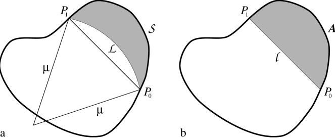
Figure 3: When $T$ is a twist map, its generating function $G$ can be expressed (a) as a function of the length ${\cal L}$ of $\gamma$ and the area ${\cal S}$ between $\gamma$ and $\partial Q$, or (b) as a function of the length $\ell$ of $P_{0}P_{1}$ and the area $A$ between $P_{0}P_{1}$ and $\partial Q$.

In order to give a physical interpretation to $G$, let us recall that the momentum, which is canonically conjugate to the position, is given by

$$\mathchoice{\mbox{\boldmath$\displaystyle\bf p$}}{\mbox{\boldmath$\textstyle\bf p$}}{\mbox{\boldmath$\scriptstyle\bf p$}}{\mbox{\boldmath$\scriptscriptstyle\bf p$}}=\frac{\partial L}{\partial\mathchoice{\mbox{\boldmath$\displaystyle\bf\dot{x}$}}{\mbox{\boldmath$\textstyle\bf\dot{x}$}}{\mbox{\boldmath$\scriptstyle\bf\dot{x}$}}{\mbox{\boldmath$\scriptscriptstyle\bf\dot{x}$}}}=m\dot{\mathchoice{\mbox{\boldmath$\displaystyle\bf x$}}{\mbox{\boldmath$\textstyle\bf x$}}{\mbox{\boldmath$\scriptstyle\bf x$}}{\mbox{\boldmath$\scriptscriptstyle\bf x$}}}+q\mathchoice{\mbox{\boldmath$\displaystyle\bf A$}}{\mbox{\boldmath$\textstyle\bf A$}}{\mbox{\boldmath$\scriptstyle\bf A$}}{\mbox{\boldmath$\scriptscriptstyle\bf A$}}=(m\dot{x}-\frac{1}{2}qBy,m\dot{y}+\frac{1}{2}qBx).$$ (17)

Thus, it would have been physically more natural to use, instead of the tangent velocity $u$, the tangent momentum

$$p=-\frac{1}{mv}\left(\mathchoice{\mbox{\boldmath$\displaystyle\bf p$}}{\mbox{\boldmath$\textstyle\bf p$}}{\mbox{\boldmath$\scriptstyle\bf p$}}{\mbox{\boldmath$\scriptscriptstyle\bf p$}}|\mathchoice{\mbox{\boldmath$\displaystyle\bf t$}}{\mbox{\boldmath$\textstyle\bf t$}}{\mbox{\boldmath$\scriptstyle\bf t$}}{\mbox{\boldmath$\scriptscriptstyle\bf t$}}(s)\right)=u+\frac{1}{2\mu}(X(s)Y^{\prime}(s)-X^{\prime}(s)Y(s)).$$ (18)

Indeed, $p$ and $s$ are conjugate since they admit as a generating function the reduced action along the arc $\gamma$:

$$F=\int_{\gamma}\left(\mathchoice{\mbox{\boldmath$\displaystyle\bf p$}}{\mbox{\boldmath$\textstyle\bf p$}}{\mbox{\boldmath$\scriptstyle\bf p$}}{\mbox{\boldmath$\scriptscriptstyle\bf p$}}|d\mathchoice{\mbox{\boldmath$\displaystyle\bf x$}}{\mbox{\boldmath$\textstyle\bf x$}}{\mbox{\boldmath$\scriptstyle\bf x$}}{\mbox{\boldmath$\scriptscriptstyle\bf x$}}\right)=mv\int_{\gamma}ds+\frac{1}{2\mu}\left(ydx-xdy\right)\;\Rightarrow\;dF=mv(p_{0}ds_{0}-p_{1}ds_{1}).$$ (19)

It is however more convenient to use $u$ instead of $p$. Green’s theorem implies that the generating functions are related by

$$mvG=F+\frac{1}{2}qB\int_{\gamma_{Q}}ydx-xdy,$$ (20)

where $\gamma_{Q}$ is the piece of boundary connecting $P_{0}$ to $P_{1}$.

One application of generating functions is in perturbation theory. Suppose the map $T_{\varepsilon}$ depends on a parameter $\varepsilon$ (controlling the magnetic field or the shape of the boundary), such that the behaviour of $T_{0}$ is known (e.g. integrable). Approximating $T_{\varepsilon}$ by its expansion $T_{0}+\varepsilon\partial_{\varepsilon}T_{\varepsilon}|_{\varepsilon=0}$ does in general not lead to an area preserving map, whereas the map generated by $G(s_{0},s_{1},0)+\varepsilon\partial_{\varepsilon}G(s_{0},s_{1},\varepsilon)|_{\varepsilon=0}$ is always conservative.

For example, the generating function for an elliptic boundary close to a circle, given by (15) with $\lambda=1+\varepsilon$, is

$$G = G_{0}(\varphi_{-})+\varepsilon G_{1}(\varphi_{+},\varphi_{-})+O(\varepsilon^{2}),$$

$$G_{0}(\varphi_{-}) = \frac{1}{\mu}\left[\varphi_{-}+\frac{1}{2}\sin(2\varphi_{-})\right]+B_{\mu}(2\sin\varphi_{-}),$$

$$G_{1}(\varphi_{+},\varphi_{-}) = \frac{1}{\mu}\left[\varphi_{-}+\frac{1}{2}\sin(2\varphi_{-})\right]+2\sin\varphi_{-}\sin^{2}\varphi_{+}\sqrt{1-\frac{\sin^{2}\varphi_{-}}{\mu^{2}}}.$$ (21)

Another use of generating functions is in searching periodic orbits. If we define the $n$-point generating function

$$G^{(n)}(s_{0},s_{1},\ldots,s_{n-1})=G(s_{0},s_{1})+G(s_{1},s_{2})+\cdots+G(s_{n-1},s_{0}),$$ (22)

then the law of specular reflection implies that every periodic orbit containing no points with $s\in E_{2}$ is a solution of

$$\frac{\partial G^{(n)}}{\partial s_{0}}=\frac{\partial G^{(n)}}{\partial s_{1}}=\ldots=\frac{\partial G^{(n)}}{\partial s_{n-1}}=0,$$ (23)

which is a system of $n$ nonlinear algebraic equations of the $n$ variables $s_{0},\ldots,s_{n-1}$.

It is convenient to “lift” the periodic variable $s$ to the real line. An $(m,n)$ periodic orbit is then defined by $s_{n}=s_{0}+m\left|\partial Q\right|,u_{n}=u_{0}$, and its frequency $\omega=\frac{1}{\left|\partial Q\right|}\lim_{k\rightarrow\infty}\frac{s_{k}}{k}$ is equal to $\frac{m}{n}$. The possible frequencies belong to an interval $I_{\omega}$, depending on the behaviour of the boundaries $u=\pm 1$ of the phase cylinder. First results on existence of periodic orbits for continuous area-preserving twist maps are due to Poincaré and Birkhoff. Powerful developments were achieved by Aubry and Le Daeron, Mather, MacKay and Meiss, and Katok (see [Me] and references therein for more details):

1. For every $m,n,\frac{m}{n}\in I_{\omega}$, there is at least one $(m,n)$ periodic orbit which is “maximizing”. This means that every finite orbit segment $(s_{k},\ldots,s_{l}),l\geq k+2$ is a global maximum of $\sum_{j=k}^{l-1}G(s_{j},s_{j+1})$ with respect to variations of $s_{k+1},\ldots,s_{l-1}$. In particular, $(s_{0},\ldots,s_{n-1})$ is a global maximum of $G^{(n)}$. If the maximum is nondegenerate, the orbit is hyperbolic.

2. For every $m,n,\frac{m}{n}\in I_{\omega}$, there is at least one $(m,n)$ periodic orbit which is “maximin”. This means that the Hessian matrix of $\sum_{j=k}^{l-1}G(s_{j},s_{j+1})$ has one single positive eigenvalue. The orbit is either elliptic or inverse hyperbolic ($\mathchoice{\mbox{$\displaystyle\rm Tr$}}{\mbox{$\textstyle\rm Tr$}}{\mbox{$\scriptstyle\rm Tr$}}{\mbox{$\scriptscriptstyle\rm Tr$}}S_{n}<-2$).

3. Every orbit on a rotational invariant circle is maximizing. For every irrational $\omega\in I_{\omega}$, there is a maximizing quasiperiodic orbit of frequency $\omega$. Its closure is either an invariant circle, or an invariant Cantor set. This result is in some sense stronger than KAM theory, since it shows the existence of quasiperiodic orbits for twist maps that are not necessarily nearly integrable.

To summarize: if the bouncing map is a continuous twist map, its generating function provides a useful tool to do perturbative as well as variational calculations. In particular, we have a lower bound on the number of periodic orbits of period $n$ (namely twice as many as there are integers $m$ coprime with $n$ such that $\frac{m}{n}\in I_{\omega}$), whose stability can be related to the second derivative of the generating function.

As we shall see in the next section, an important class of maps satisfying the twist property is given by bouncing maps of billiards with smooth, convex boundaries in low magnetic field. Many billiards’ bouncing maps however are either not twist or discontinuous. Nevertheless, generalized versions of the generating function can be useful tools in some of these cases as well, as we will see in sections 5.3 and 6.2.

5 Smooth convex boundaries

Figure 4: Trajectories in an elliptic boundary, with constant $s_{0}$ and varying $u_{0}$: (a) $\mu\geq\rho_{\mathchoice{\mbox{$\displaystyle\rm max$}}{\mbox{$\textstyle\rm max$}}{\mbox{$\scriptstyle\rm max$}}{\mbox{$\scriptscriptstyle\rm max$}}}$, (b) $\rho_{\mathchoice{\mbox{$\displaystyle\rm min$}}{\mbox{$\textstyle\rm min$}}{\mbox{$\scriptstyle\rm min$}}{\mbox{$\scriptscriptstyle\rm min$}}}<\mu<\rho_{\mathchoice{\mbox{$\displaystyle\rm max$}}{\mbox{$\textstyle\rm max$}}{\mbox{$\scriptstyle\rm max$}}{\mbox{$\scriptscriptstyle\rm max$}}}$, (c) $\mu\leq\rho_{\mathchoice{\mbox{$\displaystyle\rm min$}}{\mbox{$\textstyle\rm min$}}{\mbox{$\scriptstyle\rm min$}}{\mbox{$\scriptscriptstyle\rm min$}}}$. Trajectories with $u_{0}$ near $-1$: (d) trajectory with caustic for $\mu\geq\rho_{\mathchoice{\mbox{$\displaystyle\rm max$}}{\mbox{$\textstyle\rm max$}}{\mbox{$\scriptstyle\rm max$}}{\mbox{$\scriptscriptstyle\rm max$}}}$, (e) chaotic trajectory when $\rho_{\mathchoice{\mbox{$\displaystyle\rm min$}}{\mbox{$\textstyle\rm min$}}{\mbox{$\scriptstyle\rm min$}}{\mbox{$\scriptscriptstyle\rm min$}}}<\mu<\rho_{\mathchoice{\mbox{$\displaystyle\rm max$}}{\mbox{$\textstyle\rm max$}}{\mbox{$\scriptstyle\rm max$}}{\mbox{$\scriptscriptstyle\rm max$}}}$, (f) trajectory with caustic for $\mu\leq\rho_{\mathchoice{\mbox{$\displaystyle\rm min$}}{\mbox{$\textstyle\rm min$}}{\mbox{$\scriptstyle\rm min$}}{\mbox{$\scriptscriptstyle\rm min$}}}$.

5.1 Qualitative behaviour

We say that $\partial Q$ is smooth and convex if $\rho(s)$ is a smooth function (in a sense that we will have to specify) and is bounded by positive constants: $0<\rho_{\mathchoice{\mbox{$\displaystyle\rm min$}}{\mbox{$\textstyle\rm min$}}{\mbox{$\scriptstyle\rm min$}}{\mbox{$\scriptscriptstyle\rm min$}}}\leq\rho(s)\leq\rho_{\mathchoice{\mbox{$\displaystyle\rm max$}}{\mbox{$\textstyle\rm max$}}{\mbox{$\scriptstyle\rm max$}}{\mbox{$\scriptscriptstyle\rm max$}}}<\infty\;\forall s$. For example, for the ellipse (15), $\rho_{\mathchoice{\mbox{$\displaystyle\rm min$}}{\mbox{$\textstyle\rm min$}}{\mbox{$\scriptstyle\rm min$}}{\mbox{$\scriptscriptstyle\rm min$}}}=\lambda^{-1}$ and $\rho_{\mathchoice{\mbox{$\displaystyle\rm max$}}{\mbox{$\textstyle\rm max$}}{\mbox{$\scriptstyle\rm max$}}{\mbox{$\scriptscriptstyle\rm max$}}}=\lambda^{2}$.

Robnik and Berry [RB] proposed to classify the dynamics by comparing $\mu$ to $\rho_{\mathchoice{\mbox{$\displaystyle\rm min$}}{\mbox{$\textstyle\rm min$}}{\mbox{$\scriptstyle\rm min$}}{\mbox{$\scriptscriptstyle\rm min$}}}$ and $\rho_{\mathchoice{\mbox{$\displaystyle\rm max$}}{\mbox{$\textstyle\rm max$}}{\mbox{$\scriptstyle\rm max$}}{\mbox{$\scriptscriptstyle\rm max$}}}$. If we consider specifically the twist property, by looking at trajectories with fixed $s_{0}$ and varying $u_{0}$ (fig.4 and 5), we obtain the following “curvature regimes”:

1. If $\mu\geq\rho_{\mathchoice{\mbox{$\displaystyle\rm max$}}{\mbox{$\textstyle\rm max$}}{\mbox{$\scriptstyle\rm max$}}{\mbox{$\scriptscriptstyle\rm max$}}}$, the function $s_{1}(s_{0},u_{0})$ is increasing in $u_{0}$, so that $T$ is a twist map. The curve $\left\{T(s_{0},u_{0}),-1<u_{0}<1\right\}$ turns exactly once around the phase cylinder, with $\lim_{u_{0}\rightarrow\pm 1}T(s_{0},u_{0})=(s_{0},u_{0})$. Thus, $I_{\omega}=[0,1]$.

2. If $\rho_{\mathchoice{\mbox{$\displaystyle\rm min$}}{\mbox{$\textstyle\rm min$}}{\mbox{$\scriptstyle\rm min$}}{\mbox{$\scriptscriptstyle\rm min$}}}<\mu<\rho_{\mathchoice{\mbox{$\displaystyle\rm max$}}{\mbox{$\textstyle\rm max$}}{\mbox{$\scriptstyle\rm max$}}{\mbox{$\scriptscriptstyle\rm max$}}}$, discontinuities in the map occur when the trajectory becomes tangent to the boundary. We have $\lim_{u_{0}\rightarrow+1}T(s_{0},u_{0})=(s_{0},u_{0})$, but this is not necessarily true for $u_{0}\rightarrow-1$. In appendix C, we illustrate the construction of the discontinuity lines of the map.

3. If $\mu\leq\rho_{\mathchoice{\mbox{$\displaystyle\rm min$}}{\mbox{$\textstyle\rm min$}}{\mbox{$\scriptstyle\rm min$}}{\mbox{$\scriptscriptstyle\rm min$}}}$, the function $s_{1}(s_{0},u_{0})$ is first decreasing in $u_{0}$, reaches its minimum when $\chi=\pi/2$, and increases again. We again have $\lim_{u_{0}\rightarrow\pm 1}T(s_{0},u_{0})=(s_{0},u_{0})$, so that there are exactly two trajectories with supplementary $\chi$ for given $s_{0}$, $s_{1}$. The map is no longer twist. One can expect that the frequencies belong to an interval $I_{\omega}=[\omega_{\mathchoice{\mbox{$\displaystyle\rm min$}}{\mbox{$\textstyle\rm min$}}{\mbox{$\scriptstyle\rm min$}}{\mbox{$\scriptscriptstyle\rm min$}}},0]$, where $\omega_{\mathchoice{\mbox{$\displaystyle\rm min$}}{\mbox{$\textstyle\rm min$}}{\mbox{$\scriptstyle\rm min$}}{\mbox{$\scriptscriptstyle\rm min$}}}\sim\mu$.

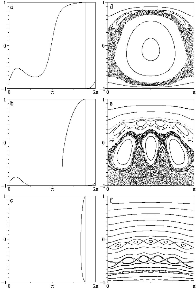
Figure 5: Structure of phase space in the $(\varphi,u)$ plane for the ellipse. Image of the line $(\varphi=\varphi^{*},-1\leq u\leq 1):$ (a) $\mu\geq\rho_{\mathchoice{\mbox{$\displaystyle\rm max$}}{\mbox{$\textstyle\rm max$}}{\mbox{$\scriptstyle\rm max$}}{\mbox{$\scriptscriptstyle\rm max$}}}$, (b) $\rho_{\mathchoice{\mbox{$\displaystyle\rm min$}}{\mbox{$\textstyle\rm min$}}{\mbox{$\scriptstyle\rm min$}}{\mbox{$\scriptscriptstyle\rm min$}}}<\mu<\rho_{\mathchoice{\mbox{$\displaystyle\rm max$}}{\mbox{$\textstyle\rm max$}}{\mbox{$\scriptstyle\rm max$}}{\mbox{$\scriptscriptstyle\rm max$}}}$, (c) $\mu\leq\rho_{\mathchoice{\mbox{$\displaystyle\rm min$}}{\mbox{$\textstyle\rm min$}}{\mbox{$\scriptstyle\rm min$}}{\mbox{$\scriptscriptstyle\rm min$}}}$. Typical phase portraits: (d) $\mu\geq\rho_{\mathchoice{\mbox{$\displaystyle\rm max$}}{\mbox{$\textstyle\rm max$}}{\mbox{$\scriptstyle\rm max$}}{\mbox{$\scriptscriptstyle\rm max$}}}$, (e) $\rho_{\mathchoice{\mbox{$\displaystyle\rm min$}}{\mbox{$\textstyle\rm min$}}{\mbox{$\scriptstyle\rm min$}}{\mbox{$\scriptscriptstyle\rm min$}}}<\mu<\rho_{\mathchoice{\mbox{$\displaystyle\rm max$}}{\mbox{$\textstyle\rm max$}}{\mbox{$\scriptstyle\rm max$}}{\mbox{$\scriptscriptstyle\rm max$}}}$, (f) $\mu\leq\rho_{\mathchoice{\mbox{$\displaystyle\rm min$}}{\mbox{$\textstyle\rm min$}}{\mbox{$\scriptstyle\rm min$}}{\mbox{$\scriptscriptstyle\rm min$}}}$.

Figures 4 and 5 illustrate this behaviour in the case of an elliptic boundary. We see that there always exist invariant curves near $u=+1$, corresponding to trajectories with caustics (the “whispering gallery modes”). For $\mu\geq\rho_{\mathchoice{\mbox{$\displaystyle\rm max$}}{\mbox{$\textstyle\rm max$}}{\mbox{$\scriptstyle\rm max$}}{\mbox{$\scriptscriptstyle\rm max$}}}$ and $\mu\leq\rho_{\mathchoice{\mbox{$\displaystyle\rm min$}}{\mbox{$\textstyle\rm min$}}{\mbox{$\scriptstyle\rm min$}}{\mbox{$\scriptscriptstyle\rm min$}}}$, such curves also exist near $u=-1$. However, when $\rho_{\mathchoice{\mbox{$\displaystyle\rm min$}}{\mbox{$\textstyle\rm min$}}{\mbox{$\scriptstyle\rm min$}}{\mbox{$\scriptscriptstyle\rm min$}}}<\mu<\rho_{\mathchoice{\mbox{$\displaystyle\rm max$}}{\mbox{$\textstyle\rm max$}}{\mbox{$\scriptstyle\rm max$}}{\mbox{$\scriptscriptstyle\rm max$}}}$, the tori near $u=-1$ are replaced by a chaotic region. This behaviour can be heuristically understood by noting the following two points: first, discontinuities of the map due to tangencies may destroy invariant curves in an analog manner as do the discontinuities due to corners of the boundary [DR]; second, the Jacobian matrix (3) diverges like $(u+1)^{-1/2}$, causing strong dispersion of nearly tangent orbits, which can be a source of positive Liapunov exponents.

Robnik and Berry have computed an adiabatic invariant, which tends to be conserved if $\left|\frac{\kappa\mu\sqrt{1-u^{2}}}{1+\kappa\mu u}\right|\ll 1$:

$$K(s,u)=\frac{\mu\kappa(s)+u(3-2u^{2})}{(1-u^{2})^{3/2}},$$ (24)

and gives a very good approximation of the invariant curves for $u\rightarrow\pm 1$. As it turns out, in the strong field limit $\mu\kappa\ll 1$, $K$ tends to be conserved for all orbits, so that this limit seems to be integrable. In the following, our aim is to delineate the validity of these statements and make them more precise by using different perturbative approaches.

5.2 Near the boundary

We recall that for Euclidean billiards, the existence of invariant curves and caustics near the boundary was first demonstrated by Lazutkin [L], who had to assume a high degree of differentiability. Douady [Do] reduced the required degree to 6. On the other hand, Hubacher [H] proved that no caustics exist near a boundary whose curvature is discontinuous, and Mather [Ma] found that if the curvature of the boundary vanishes at one point, then invariant curves are totally absent.

We are now going to investigate the behaviour of the bouncing map of billiards in non-zero magnetic field near their boundary, i.e. for small $\sin\theta_{0}$. In this way, we will be able to apply KAM theorems to show the existence of invariant curves. The results are summarized in theorem 1 at the end of this section.

If we write $z(s)=X(s)+\mathchoice{\mbox{$\displaystyle\rm i$}}{\mbox{$\textstyle\rm i$}}{\mbox{$\scriptstyle\rm i$}}{\mbox{$\scriptscriptstyle\rm i$}}Y(s)$, and $z_{i}=z(s_{i})$, $\tau_{i}=\tau(s_{i})$, we have

$$z_{1}-z_{0}=\int_{s_{0}}^{s_{1}}\mathchoice{\mbox{$\displaystyle\rm e$}}{\mbox{$\textstyle\rm e$}}{\mbox{$\scriptstyle\rm e$}}{\mbox{$\scriptscriptstyle\rm e$}}^{\mathchoice{\mbox{$\displaystyle\rm i$}}{\mbox{$\textstyle\rm i$}}{\mbox{$\scriptstyle\rm i$}}{\mbox{$\scriptscriptstyle\rm i$}}\tau(s)}ds=\int_{\tau_{0}}^{\tau_{1}}\rho(\tau)\mathchoice{\mbox{$\displaystyle\rm e$}}{\mbox{$\textstyle\rm e$}}{\mbox{$\scriptstyle\rm e$}}{\mbox{$\scriptscriptstyle\rm e$}}^{\mathchoice{\mbox{$\displaystyle\rm i$}}{\mbox{$\textstyle\rm i$}}{\mbox{$\scriptstyle\rm i$}}{\mbox{$\scriptscriptstyle\rm i$}}\tau}d\tau.$$ (25)

Since the $z_{i}$ also belong to the arc of trajectory, which has tangent directions $\tau_{0}+\theta_{0}$ at $z_{0}$ and $\tau_{1}-\theta_{1}$ at $z_{1}$ (see fig.2), we have

$$z_{1}-z_{0}=\frac{\mu}{\mathchoice{\mbox{$\displaystyle\rm i$}}{\mbox{$\textstyle\rm i$}}{\mbox{$\scriptstyle\rm i$}}{\mbox{$\scriptscriptstyle\rm i$}}}\left[\mathchoice{\mbox{$\displaystyle\rm e$}}{\mbox{$\textstyle\rm e$}}{\mbox{$\scriptstyle\rm e$}}{\mbox{$\scriptscriptstyle\rm e$}}^{\mathchoice{\mbox{$\displaystyle\rm i$}}{\mbox{$\textstyle\rm i$}}{\mbox{$\scriptstyle\rm i$}}{\mbox{$\scriptscriptstyle\rm i$}}(\tau_{1}-\theta_{1})}-\mathchoice{\mbox{$\displaystyle\rm e$}}{\mbox{$\textstyle\rm e$}}{\mbox{$\scriptstyle\rm e$}}{\mbox{$\scriptscriptstyle\rm e$}}^{\mathchoice{\mbox{$\displaystyle\rm i$}}{\mbox{$\textstyle\rm i$}}{\mbox{$\scriptstyle\rm i$}}{\mbox{$\scriptscriptstyle\rm i$}}(\tau_{0}+\theta_{0})}\right].$$ (26)

Introducing $A=\mathchoice{\mbox{$\displaystyle\rm e$}}{\mbox{$\textstyle\rm e$}}{\mbox{$\scriptstyle\rm e$}}{\mbox{$\scriptscriptstyle\rm e$}}^{-\mathchoice{\mbox{$\displaystyle\rm i$}}{\mbox{$\textstyle\rm i$}}{\mbox{$\scriptstyle\rm i$}}{\mbox{$\scriptscriptstyle\rm i$}}\tau_{0}}(z_{1}-z_{0})$ and $\delta=\tau_{1}-\tau_{0}-\theta_{1}+\theta_{0}$, this can be rewritten

$$A-\mu\mathchoice{\mbox{$\displaystyle\rm e$}}{\mbox{$\textstyle\rm e$}}{\mbox{$\scriptstyle\rm e$}}{\mbox{$\scriptscriptstyle\rm e$}}^{-\mathchoice{\mbox{$\displaystyle\rm i$}}{\mbox{$\textstyle\rm i$}}{\mbox{$\scriptstyle\rm i$}}{\mbox{$\scriptscriptstyle\rm i$}}\theta_{0}}\frac{\mathchoice{\mbox{$\displaystyle\rm e$}}{\mbox{$\textstyle\rm e$}}{\mbox{$\scriptstyle\rm e$}}{\mbox{$\scriptscriptstyle\rm e$}}^{\mathchoice{\mbox{$\displaystyle\rm i$}}{\mbox{$\textstyle\rm i$}}{\mbox{$\scriptstyle\rm i$}}{\mbox{$\scriptscriptstyle\rm i$}}\delta}-1}{\mathchoice{\mbox{$\displaystyle\rm i$}}{\mbox{$\textstyle\rm i$}}{\mbox{$\scriptstyle\rm i$}}{\mbox{$\scriptscriptstyle\rm i$}}}=-2\mu\sin\theta_{0},$$ (27)

which is equivalent to the system

$$\frac{\mathchoice{\mbox{$\displaystyle\rm Re$}}{\mbox{$\textstyle\rm Re$}}{\mbox{$\scriptstyle\rm Re$}}{\mbox{$\scriptscriptstyle\rm Re$}}A}{\sin\theta_{0}}-\mu\cos\theta_{0}\frac{\sin\delta}{\sin\theta_{0}}+\mu(\cos\delta-1) = -2\mu$$

$$\frac{\mathchoice{\mbox{$\displaystyle\rm Im$}}{\mbox{$\textstyle\rm Im$}}{\mbox{$\scriptstyle\rm Im$}}{\mbox{$\scriptscriptstyle\rm Im$}}A}{\sin^{2}\theta_{0}}+\mu\frac{\sin\delta}{\sin\theta_{0}}+\mu\cos\theta_{0}\frac{\cos\delta-1}{\sin^{2}\theta_{0}} = 0.$$ (28)

If the boundary is $C^{k}$, this is a system of $C^{k-1}$ equations in the variables $s_{0},\theta_{0},s_{1},\theta_{1}$ that we would like to solve with respect to $s_{1},\theta_{1}$.

Writing $s_{1}=s_{0}+\sin\theta_{0}\mu\sigma$ and $\theta_{1}=\theta_{0}+\sin\theta_{0}\mu\gamma$, we obtain for $k\geq 3$

$$A = \sin\theta_{0}\mu\sigma+\frac{\mathchoice{\mbox{$\displaystyle\rm i$}}{\mbox{$\textstyle\rm i$}}{\mbox{$\scriptstyle\rm i$}}{\mbox{$\scriptscriptstyle\rm i$}}}{2}\sin^{2}\theta_{0}\mu^{2}\sigma^{2}\kappa(s_{0})+O(\mu^{3}\sin^{3}\theta_{0})$$

$$\delta = \sin\theta_{0}\mu\left[\kappa(s_{0})\sigma-\gamma\right]+O(\mu^{2}\sin^{2}\theta_{0}).$$ (29)

Replacing this in (28) finally leads to the system

$$\sigma-\mu\cos\theta_{0}\left[\kappa(s_{0})\sigma-\gamma\right]+O(\sin\theta_{0}) = -2$$

$$\sigma^{2}\kappa(s_{0})+2\left[\kappa(s_{0})\sigma-\gamma\right]-\mu\cos\theta_{0}\left[\kappa(s_{0})\sigma-\gamma\right]^{2}+O(\sin\theta_{0}) = 0,$$ (30)

which has the solution

$$\sigma(s_{0},\theta_{0},\mu) = \frac{-2}{1-\mu\cos\theta_{0}\kappa(s_{0})}+O(\sin\theta_{0})$$

$$\gamma(s_{0},\theta_{0},\mu) = O(\sin\theta_{0}).$$ (31)

Since the Jacobian of (30) evaluated at this solution is $-2+O(\sin\theta_{0})$, the implicit function theorem implies that for small $\sin\theta_{0}$, the bouncing map is $C^{k-1}$ and has the form

$$s_{1} = s_{0}-\frac{2\mu\sin\theta_{0}}{1-\mu\cos\theta_{0}\kappa(s_{0})}+o(\sin\theta_{0})\pmod{\left|\partial Q\right|}$$

$$\theta_{1} = \theta_{0}+o(\sin\theta_{0}).$$ (32)

However, this formula is only valid if we are able to check two properties: firstly, the approximation must be well defined, i.e. the denominator in the first equation should not vanish. Secondly, the solution (31) has to be the “right” one, that is the first intersection of the trajectory with the boundary, following the motion of the particle. We have to distinguish between the following cases:

1. Near $u=+1$: Writing $\theta=\pi-\eta$, (32) becomes

   $$s_{1} = s_{0}-\frac{2\mu}{1+\mu\kappa(s_{0})}\eta_{0}+o(\eta_{0})\pmod{\left|\partial Q\right|}$$

   $$\eta_{1} = \eta_{0}+o(\eta_{0}).$$ (33)

   Here the denominator can never vanish. Moreover, this solution corresponds geometrically to a short skip of the particle backwards along the boundary, so that it certainly describes the first encounter of the trajectory with $\partial Q$.

   Note that this equation is well defined even when the curvature is allowed to vanish. Only when $\mu=\infty$, the first equation becomes $s_{1}=s_{0}-\frac{2}{\kappa(s_{0})}\eta_{0}+o(\eta_{0})$, and diverges when $\kappa\rightarrow 0$, which is coherent with Mather’s result.

   The change of variables $\varphi=s+\mu\tau(s)$, $r=2\mu\eta$ is well defined and transforms the map into

   $$\varphi_{1} = \varphi_{0}-r_{0}+o(r_{0})\pmod{\left|\partial Q\right|+2\pi\mu}$$

   $$r_{1} = r_{0}+o(r_{0}).$$ (34)

2. Near $u=-1$: The map has the form

   $$s_{1} = s_{0}-\frac{2\mu}{1-\mu\kappa(s_{0})}\theta_{0}+o(\theta_{0})\pmod{\left|\partial Q\right|}$$

   $$\theta_{1} = \theta_{0}+o(\theta_{0}).$$ (35)

   This time, we have to be careful with the denominator, which may vanish. The approximation $\theta\ll 1$ is only valid in two cases:

   1. If $\mu\geq\rho_{\mathchoice{\mbox{$\displaystyle\rm max$}}{\mbox{$\textstyle\rm max$}}{\mbox{$\scriptstyle\rm max$}}{\mbox{$\scriptscriptstyle\rm max$}}}(1+\varepsilon)$, $\varepsilon>0$, then in the variables $\varphi=\mu\tau(s)-s$, $r=2\mu\theta$, the map becomes

      $$\varphi_{1} = \varphi_{0}+r_{0}+o(r_{0})\pmod{2\pi\mu-\left|\partial Q\right|}$$

      $$r_{1} = r_{0}+o(r_{0}).$$ (36)

      We again got the right intersection, because the particle is skipping forward along the boundary (fig.4d).

   2. If $\mu\leq\rho_{\mathchoice{\mbox{$\displaystyle\rm min$}}{\mbox{$\textstyle\rm min$}}{\mbox{$\scriptstyle\rm min$}}{\mbox{$\scriptscriptstyle\rm min$}}}(1-\varepsilon)$, then in the variables $\varphi=s-\mu\tau(s)$, $r=2\mu\theta$, the map reads

      $$\varphi_{1} = \varphi_{0}-r_{0}+o(r_{0})\pmod{\left|\partial Q\right|-2\pi\mu}$$

      $$r_{1} = r_{0}+o(r_{0}).$$ (37)

      This time, the particle is starting with a forward glancing velocity, but reaches the boundary behind its starting point (fig.4f). It is not obvious that there is not another intersection of the trajectory and the boundary in between. Luckily, lemma 3 in appendix D shows that this cannot happen, because any circle of radius $\mu<\rho_{\mathchoice{\mbox{$\displaystyle\rm min$}}{\mbox{$\textstyle\rm min$}}{\mbox{$\scriptstyle\rm min$}}{\mbox{$\scriptscriptstyle\rm min$}}}$ cuts $\partial Q$ at two points at most.

The maps (34), (36) and (37) can now be treated by KAM-type theorems ([Mo], p.52 or [Do], p.III-8). In this way, we obtain the following result:

Theorem 1 Consider a magnetic billiard in a domain with $C^{k}$ boundary, $k\geq 6$, such that $0<\rho_{\mathchoice{\mbox{$\displaystyle\rm min$}}{\mbox{$\textstyle\rm min$}}{\mbox{$\scriptstyle\rm min$}}{\mbox{$\scriptscriptstyle\rm min$}}}\leq\rho(s)\leq\rho_{\mathchoice{\mbox{$\displaystyle\rm max$}}{\mbox{$\textstyle\rm max$}}{\mbox{$\scriptstyle\rm max$}}{\mbox{$\scriptscriptstyle\rm max$}}}\leq\infty$. Let $\varepsilon\in{\rm I\!R}_{+}^{*}$ and assume that one of the following is true

1. $0<\mu<\infty$, $\eta=\pi-\theta$, $L=\left|\partial Q\right|+2\pi\mu$, $\sigma=-1$;

2. $\rho_{\mathchoice{\mbox{$\displaystyle\rm max$}}{\mbox{$\textstyle\rm max$}}{\mbox{$\scriptstyle\rm max$}}{\mbox{$\scriptscriptstyle\rm max$}}}(1+\varepsilon)\leq\mu<\infty$, $\eta=\theta$, $L=2\pi\mu-\left|\partial Q\right|$, $\sigma=+1$;

3. $0<\mu\leq\rho_{\mathchoice{\mbox{$\displaystyle\rm min$}}{\mbox{$\textstyle\rm min$}}{\mbox{$\scriptstyle\rm min$}}{\mbox{$\scriptscriptstyle\rm min$}}}(1-\varepsilon)$, $\eta=\theta$, $L=\left|\partial Q\right|-2\pi\mu$, $\sigma=-1$.

Then, there exists $\varepsilon_{1}>0$ (depending on $\mu$ and $k$) such that, if $\omega\in[0,\varepsilon_{1})$ and satisfies the diophantine conditions

$$\left|\frac{\omega}{L}-\frac{p}{q}\right|\geq\gamma q^{-\nu}$$ (38)

for some $\gamma,\nu\in{\rm I\!R}_{+}^{*}$ and for any $\frac{p}{q}\in{\mathchoice{\hbox{\raise 1.02495pt\hbox to0.0pt{\kern 3.11107pt\vrule height=5.46666pt\hss}\hbox{$\displaystyle\rm Q$}}}{\hbox{\raise 1.02495pt\hbox to0.0pt{\kern 3.11107pt\vrule height=5.46666pt\hss}\hbox{$\textstyle\rm Q$}}}{\hbox{\raise 0.71747pt\hbox to0.0pt{\kern 2.17775pt\vrule height=3.34831pt\hss}\hbox{$\scriptstyle\rm Q$}}}{\hbox{\raise 0.51247pt\hbox to0.0pt{\kern 1.55553pt\vrule height=2.39165pt\hss}\hbox{$\scriptscriptstyle\rm Q$}}}}$, there is an invariant curve of the form

$$s = \xi+V(\xi)$$

$$\eta = \frac{\omega}{2\mu}+U(\xi),$$ (39)

where $U,V\in C^{1}$, $V(\xi+L)=V(\xi)+\left|\partial Q\right|-L$, $U(\xi+L)=U(\xi)$. The induced map on this curve has the form

$$\xi\mapsto\xi+\sigma\omega.$$ (40)

This theorem confirms our observation that invariant curves exist in three cases:

1. Near $u=+1,\;(\theta=\pi)$, for all values of the magnetic field (see the upper parts of fig.5d-f). They correspond to backward skipping trajectories, the curvature of which is opposite to the curvature of the boundary.

2. Near $u=-1,\;(\theta=0)$, in weak magnetic field ($\mu\geq\rho_{\mathchoice{\mbox{$\displaystyle\rm max$}}{\mbox{$\textstyle\rm max$}}{\mbox{$\scriptstyle\rm max$}}{\mbox{$\scriptscriptstyle\rm max$}}}(1+\varepsilon)$, see the lower part of fig.5d). They correspond to forward skipping trajectories (fig.4d), which are curved away from the boundary.

3. Near $u=-1,\;(\theta=0)$, in strong magnetic field ($\mu\leq\rho_{\mathchoice{\mbox{$\displaystyle\rm min$}}{\mbox{$\textstyle\rm min$}}{\mbox{$\scriptstyle\rm min$}}{\mbox{$\scriptscriptstyle\rm min$}}}(1-\varepsilon)$, see the lower part of fig.5f). They correspond to backward skipping trajectories (fig.4f).

For intermediate values of the magnetic field, there seem to be no tori near $u=-1$. Although we have a qualitative understanding of the origin of this phenomenon, we are not able to prove the existence of a stochastic component of positive measure in this region. This remains an open problem.

On the other hand, our theorem implies that magnetic billiards in smooth (i.e. $C^{6}$) convex domains can never be ergodic. Unlike in zero field, this remains true even when the curvature of the boundary is allowed to vanish. In fact, equation (33) suggests that invariant curves exist near $u=+1$ even when the boundary has slightly concave parts, i.e. $\kappa(s)\geq-\kappa_{0}$, $\kappa_{0}>0$, and for $\mu\leq\frac{1}{\kappa_{0}}-\varepsilon$. In that case, however, the tori near $u=-1$ do not necessarily survive. We will come back to that point in section 6.2.

5.3 The strong field limit

The limit $\mu\rightarrow 0$ is in some sense singular: indeed, for small $\mu$, the distance between successive collisions with the boundary is of order $\mu$, so that one could get the impression that the particle follows the boundary more and more slowly when $\mu$ decreases, and sticks to the wall when $\mu=0$, violating the conservation of energy. Of course, this is only an artificial effect, due to the fact that we use the bouncing map instead of the flow to describe the dynamics. Indeed, the “time of flight” between successive collisions is also of order $\mu$ (more precisely, it is equal to $\mu\psi$, where $\psi$ is given in fig.2), so that during a given time interval, the particle hits the boundary $O(1/\mu)$ times, traveling a finite distance.

Thus, we have to be careful when we apply perturbation theory. It is possible to use (28) to analyze the limit $\mu\rightarrow 0$. However, we give in appendix D an alternative approach that we find more instructive. The idea is to show that although the map is not twist, it can be described by generating functions, in fact two of them, with suitable matching at $\chi=\pi/2$. These functions are of the form $G^{\pm}(s_{0},s_{1},\mu)=\pm\mu g_{0}(\sigma)+\mu^{2}g_{1}^{\pm}(\sigma,s_{0},\mu)$, where $\sigma=\frac{s_{0}-s_{1}}{\mu}$. Replacing this in (10), we see that $\sigma$ and $u$ are “slow” variables which evolve on a much longer time scale than $s$. This expresses the geometrical idea that for a short skip, the boundary is close to an arc of circle, for which $\sigma$ and $u$ are constants. It is however necessary to use the variable $\theta$ instead of $u$ if we wish that the map be smooth at the boundaries of the phase cylinder. Finally, we obtain the following result:

Proposition 3 Consider a magnetic billiard with a convex, $C^{k}$ boundary, $k\geq 3$. For small enough $\mu$, the bouncing map is $C^{k-1}$ and has the form:

$$s_{1} = s_{0}-2\mu\sin\theta_{0}+\mu^{2}\sin\theta_{0}\,a(s_{0},\theta_{0},\mu)\pmod{\left|\partial Q\right|},$$

$$\theta_{1} = \theta_{0}+\mu^{2}\sin^{2}\theta_{0}\,b(s_{0},\theta_{0},\mu).$$ (41)

The functions $a\in C^{k-2}$ and $b\in C^{k-3}$ are uniformly bounded for $s\in{\rm I\!R},0\leq\theta\leq\pi$, $\left|\partial Q\right|$-periodic in $s$, and admit the expansions

$$a(s,\theta,\mu) = \sum_{i=0}^{k-3}a_{i}(s,\theta)\mu^{i}+O(\mu^{k-2}),$$

$$b(s,\theta,\mu) = \sum_{j=0}^{k-4}b_{j}(s,\theta)\mu^{j}+O(\mu^{k-3})\;\;\;(k\geq 4),$$ (42)

where the first terms are

$$a_{0} = -2\cos\theta\kappa(s),$$

$$a_{1} = -\frac{2}{3}\left[(1+2\cos 2\theta)\kappa(s)^{2}-\sin 2\theta\,\kappa^{\prime}(s)\right],$$

$$b_{0} = \frac{2}{3}\kappa^{\prime}(s),$$

$$b_{1} = \frac{4}{3}\cos\theta\kappa(s)\kappa^{\prime}(s)-\frac{2}{3}\sin\theta\kappa^{\prime\prime}(s).$$ (43)

Equation (41) shows that the bouncing map in strong magnetic field behaves like a perturbed integrable map. To zeroth order in $\mu$, it reduces to identity. To first order in $\mu$, it still has the integrable form $\theta_{1}=\theta_{0},\,s_{1}=s_{0}+\mu\Omega(\theta_{0})$, where $\Omega(\theta)=-2\sin\theta$. However, in contrast with usual integrable systems, the frequency $\Omega$ is multiplied with the small parameter $\mu$. As for the factors $\sin\theta$ occurring in (41), they assure that the boundaries $\theta=0,\,\pi$ are fixed.

The behaviour when $\mu\rightarrow 0$ can be understood in the following way: fix some positive $\mu_{0}$ and define $s=\mu_{0}\varphi$, $\tilde{a}(\varphi,\theta,\mu)=a(\mu_{0}\varphi,\theta,\mu)$, $\tilde{b}(\varphi,\theta,\mu)=b(\mu_{0}\varphi,\theta,\mu)$. Consider the 2-parameter family of maps $T_{\mu_{0},\mu}$:

$$\varphi_{1} = \varphi_{0}-2\sin\theta_{0}+\mu\sin\theta_{0}\,\tilde{a}(\varphi_{0},\theta_{0},\mu)\pmod{\frac{\left|\partial Q\right|}{\mu_{0}}},$$

$$\theta_{1} = \theta_{0}+\mu^{2}\sin^{2}\theta_{0}\,\tilde{b}(\varphi_{0},\theta_{0},\mu).$$ (44)

The map $T_{\mu_{0},0}$ is integrable, $\theta$ being a constant of motion, and it takes about $n(\theta)=\frac{\left|\partial Q\right|}{2\mu_{0}\sin\theta}$ iterations for $\varphi$ to turn once around phase space. $T_{\mu_{0},\mu_{0}}$ is equivalent to (41), and one can expect that when $\mu_{0}$ is small, some features of the integrable map remain, in particular the particle completes one turn after roughly $n(\theta)$ bounces. Using (80) and (41), we obtain that $\psi=2\chi=2\pi-2\theta_{0}+O(\mu)$, so that the time necessary for one revolution is of order $t\sim n(\theta)\mu_{0}\psi\sim\left|\partial Q\right|\frac{\pi-\theta}{\sin\theta}$, which does not depend on $\mu$ to lowest order. Note an important difference between the skipping regimes $u\sim+1$ and $u\sim-1$: in the first case, $t\sim\left|\partial Q\right|$, whereas in the second case $t\sim\left|\partial Q\right|\frac{\pi}{\theta}$ diverges when $u\rightarrow-1$. The variation of $\theta$ during $t$ is of order $n(\theta)(\theta_{1}-\theta_{0})\sim\mu_{0}\sin\theta$, which shows that our approximation is consistent, since $\theta$ is an adiabatic invariant on the time scale $t$.

We have the choice between two different perturbative techniques to make these observations mathematically precise. If we exclude some neighborhood of $\theta=\frac{\pi}{2}$, where the frequency $\Omega(\theta)=-2\sin\theta$ has a vanishing derivative, we can apply Moser’s theorem ([Mo], p.52): if the boundary is $C^{k},k\geq 6$, then there exist invariant curves for every frequency satisfying some diophantine condition. In this way however, we cannot describe trajectories starting with a very small tangential velocity ($\theta\sim\frac{\pi}{2}$). In order to do this, we will apply another technique to study (41), coming from adiabatic theory. We will prove in section 7 the following theorem on a class of maps of the annulus:

Theorem 2 (An adiabatic theorem for maps)

Let the map $T:(\varphi_{0},I_{0},\mu)\mapsto(\varphi_{1},I_{1})$,

$$\varphi_{1} = \varphi_{0}+\mu c(I_{0})\left[\Omega(I_{0},\mu)+\mu\alpha(\varphi_{0},I_{0},\mu)\right]$$

$$I_{1} = I_{0}+\mu^{2}c(I_{0})^{2}\beta(\varphi_{0},I_{0},\mu),$$ (45)

be defined on the set $E=\left\{(\varphi,I,\mu)\mid\varphi\in{\rm I\!R},0\leq I\leq 1,0\leq\mu\leq\mu^{*}\right\}$. Assume that $\alpha$ and $\beta$ are periodic functions of $\varphi$ with period $1$, $c(0)=c(1)=0$, and $\Omega(I,0)=\Omega_{0}\neq 0$.

Then, there exists a change of variables $(\varphi,I)\mapsto(\psi=\varphi+\mu f(\varphi,I,\mu),J=I+\mu c(I)g(\varphi,I,\mu))$, preserving the square $[0,1]\times[0,1]$, where $f$ and $g$ are periodic with period $1$ in $\varphi$, such that

1. If $T$ is analytic in a complex neighborhood of $E$, then

   $$\psi_{1} = \psi_{0}+\mu c(J_{0})\left[\bar{\Omega}(J_{0},\mu)+\mathchoice{\mbox{$\displaystyle\rm e$}}{\mbox{$\textstyle\rm e$}}{\mbox{$\scriptstyle\rm e$}}{\mbox{$\scriptscriptstyle\rm e$}}^{-1/C\mu}\bar{\alpha}(\psi_{0},J_{0},\mu)\right]$$

   $$J_{1} = J_{0}+\mu^{2}c(J_{0})^{2}\left[\Theta(J_{0},\mu)+\mathchoice{\mbox{$\displaystyle\rm e$}}{\mbox{$\textstyle\rm e$}}{\mbox{$\scriptstyle\rm e$}}{\mbox{$\scriptscriptstyle\rm e$}}^{-1/C\mu}\bar{\beta}(\psi_{0},J_{0},\mu)\right].$$ (46)

2. If moreover $T$ preserves the measure $c(I)\rho(\varphi,I,\mu)d\varphi dI$, where $\rho(\varphi,I,0)=1$, then

   $$J_{1}=J_{0}+\mathchoice{\mbox{$\displaystyle\rm e$}}{\mbox{$\textstyle\rm e$}}{\mbox{$\scriptstyle\rm e$}}{\mbox{$\scriptscriptstyle\rm e$}}^{-1/C\mu}c(J_{0})^{2}\bar{\beta}(\psi_{0},J_{0},\mu).$$ (47)

3. If $\alpha$, $\beta$ and $\Omega$ are $C^{k}$ and $c$ is $C^{k+1}$ in $E$, then

   $$\psi_{1} = \psi_{0}+\mu c(J_{0})\left[\bar{\Omega}(J_{0},\mu)+\mu^{k+1}\bar{\alpha}(\psi_{0},J_{0},\mu)\right]$$

   $$J_{1} = J_{0}+\mu^{2}c(J_{0})^{2}\left[\Theta(J_{0},\mu)+\mu^{k}\bar{\beta}(\psi_{0},J_{0},\mu)\right],$$ (48)

   respectively

   $$J_{1}=J_{0}+\mu^{k+2}c(J_{0})^{2}\bar{\beta}(\psi_{0},J_{0},\mu)$$ (49)

   if $T$ preserves the measure $c(I)\rho(\varphi,I,\mu)d\varphi dI$.

Equation (45) describes a map from the annulus $0\leq I\leq 1$ into itself (the choice of 0, 1, is arbitrary and can be changed by scaling). Indeed, the factor $c(I)$, which vanishes at $I=0,\,1$, assures that the boundaries of the annulus are fixed, and for small enough $\mu$, the interior of the annulus is invariant. In (45), the terms containing the phase $\varphi$, which make the map non-integrable, are of order $\mu^{2}$. The theorem states that a suitable change of variables decreases this order to $\mu^{k+2}$ if the map is $C^{k}$, and to the exponentially small order $\mathchoice{\mbox{$\displaystyle\rm e$}}{\mbox{$\textstyle\rm e$}}{\mbox{$\scriptstyle\rm e$}}{\mbox{$\scriptscriptstyle\rm e$}}^{-1/C\mu}$ if the map is analytic.

The method of the proof is similar to that used by Nehoroshev and Neishtadt (see [A2], p.163 and references therein) in the case of differential equations. The basic idea is to make successive changes of variables that each decrease by one unit the order of the terms containing the phase $\varphi$. If the map is $C^{k}$, one can repeat this procedure $k$ times. If it is analytic, divergence prevents us from applying the procedure infinitely often, but it is possible to do it a large number of times, of order $\frac{1}{\mu}$, so that the terms containing the phase become exponentially small.

We can now apply the theorem to the bouncing map (41) of billiards in strong magnetic field, where $c(\theta)=\sin\theta$. Because of proposition 1, the map preserves the measure $\sin\theta dsd\theta$, and can thus be transformed into the form (47) or (49). If we write $J_{i}=J(s_{i},\theta_{i})$, we obtain

Corollary Consider a magnetic billiard in a convex domain. If the boundary is $C^{k},k\geq 3$, then there exists a function $J^{(k)}(s,\theta)$ such that $J^{(k)}_{1}=J^{(k)}_{0}+O(\mu^{k-1})$. If the boundary is analytic (in the sense that $\kappa(s)$ can be analytically continued to a complex neighborhood of the real axis), then there exists a function $J(s,\theta)$ such that $J_{1}=J_{0}+O(\mathchoice{\mbox{$\displaystyle\rm e$}}{\mbox{$\textstyle\rm e$}}{\mbox{$\scriptstyle\rm e$}}{\mbox{$\scriptscriptstyle\rm e$}}^{-1/C\mu})$. In any case, this function can be written in the form $J=\theta+\mu\sin\theta g(s,\theta,\mu)$.

If the boundary is $C^{k},k\geq 3$, this result implies that after $n$ bounces, we have $J_{n}=J_{0}+nO(\mu^{k-1})$, and hence if $n=O(\mu^{2-k})$, $J_{n}=J_{0}+O(\mu)$. In other words, the quantity $J$ is a “quasi-invariant” or “adiabatic invariant” which varies of an amount of order $\mu$ for $O(\mu^{2-k})$ bounces, i.e. during a time of order $\mu^{3-k}$. In the analytic case, $J$ varies on a time scale growing exponentially with the magnetic field. In contrast with KAM theorems, which show the existence of exact invariants for some initial conditions, the adiabatic theorem shows the existence of approximate invariants for all initial conditions.

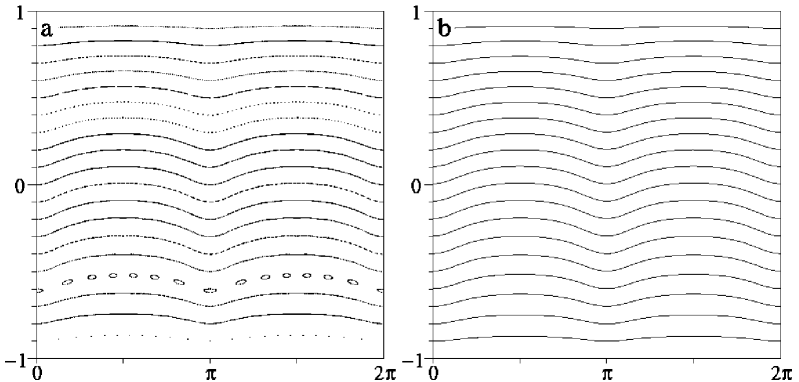
Figure 6: Adiabatic invariant in the strong field limit: (a) some orbits of the billiard in an ellipse for $\mu=0.3$, $\lambda=1.5$ (i.e. $\rho_{\mathchoice{\mbox{$\displaystyle\rm min$}}{\mbox{$\textstyle\rm min$}}{\mbox{$\scriptstyle\rm min$}}{\mbox{$\scriptscriptstyle\rm min$}}}=\frac{2}{3}$), (b) level lines of the adiabatic invariant (50), which are given by $\theta=J-\mu\sin J\left[\frac{1}{3}\kappa(s)+\frac{1}{9}\mu\cos J\kappa(s)^{2}\right]+O(\mu^{3})$.

In fact, the theorem not only shows the existence of quasi-invariants, it also enables us to compute them up to the first orders. For example, after 2 changes of variables (given by (52), (53) and (54)), we obtain

$$J^{(5)}(s,\theta,\mu)=\theta+\mu\sin\theta\left[\frac{1}{3}\kappa(s)+\frac{2}{9}\mu\cos\theta\kappa(s)^{2}\right].$$ (50)

To zeroth order in $\mu$, we recover that $J^{(3)}=\theta$ is an adiabatic invariant on a time scale of order 1. To first order in $\mu$, $J^{(4)}$ corresponds to the invariant (24) of [RB], which is valid for a time of order $\mu^{-1}$. As shown in figure 6, the orbits are very close to the level lines of $J^{(5)}$, even when $\mu$ is of the same order as $\rho_{\mathchoice{\mbox{$\displaystyle\rm min$}}{\mbox{$\textstyle\rm min$}}{\mbox{$\scriptstyle\rm min$}}{\mbox{$\scriptscriptstyle\rm min$}}}$. The dynamics on the quasi-invariant curve $J(s,\theta)=J_{0}$ is approximated by $\psi_{1}=\psi_{0}+\mu c(J_{0})\bar{\Omega}(J_{0},\mu)$.

In section 6.2, we will say a word on adiabatic invariants for billiards in non-convex boundaries. Quasi-invariants can also be used to study billiards with piecewise smooth boundaries. As long as the particle hits the same smooth piece of the boundary, the corresponding quasi-invariant changes slowly, so that one can estimate the outcoming velocity. However, as soon as the particle passes from one smooth piece to another one, a jump of the value of $J$ occurs. This is particularly clear in the stadium, where $J=\theta$ is even an exact invariant on each straight line and arc of circle. The jumps of $\theta$ occurring at the junction points allow the particle to explore a large fraction of phase space (see also [Ro]). Thus, billiards in insufficiently smooth, convex domains do not become integrable in the strong field limit (as suggested in [MBG]).

6 More chaotic billiards

Figure 7: Periodic trajectories in a square.Trajectories of period 4: (a) type I, (b) type II, (c) type III, (d) asymmetric trajectory at $\mu=0.502$, bifurcating with type I at $\mu=\frac{1}{2}$. (e) Trajectory of period 12 which bifurcates with type I when $\mu=\frac{\sqrt{5}}{2}$. (f) Stable symmetric trajectory of period $4k$, $k=2$ for $\mu=\frac{1}{4}$.

6.1 The billiard in a square

Billiards in convex polygonal domains, in the presence of a magnetic field, can be expected to show a chaotic tendency, because we will always be in the regime $0=\rho_{\mathchoice{\mbox{$\displaystyle\rm min$}}{\mbox{$\textstyle\rm min$}}{\mbox{$\scriptstyle\rm min$}}{\mbox{$\scriptscriptstyle\rm min$}}}<\mu<\rho_{\mathchoice{\mbox{$\displaystyle\rm max$}}{\mbox{$\textstyle\rm max$}}{\mbox{$\scriptstyle\rm max$}}{\mbox{$\scriptscriptstyle\rm max$}}}=\infty$.

We have concentrated our study to the case of a square of side length $1$. This billiard is integrable in zero field, where every periodic orbit is parabolic. In fact, the periodic orbits occur in families, which can be indexed by the slope of the trajectory, and whose members can be indexed by the arclength of any collision with the boundary.

In low magnetic field, only isolated orbits subsist, some of which are hyperbolic, and some elliptic (fig.8a). When the field increases, most of the latter vanish or get unstable, and structure of phase space is dominated by symmetric period-4 orbits (fig.7a-c): type I exists for $\mu\geq\frac{1}{\sqrt{8}}$, type II for $\mu>\frac{1}{2}$, and type III for $\frac{1}{\sqrt{8}}\leq\mu<\frac{1}{2}$.

Using (3), we find that type II and III orbits are hyperbolic, except for $\mu=\frac{1}{\sqrt{8}}$, where type III and type I undergo saddle-node bifurcation. For type I orbits, we find that the stability matrix satisfies

$$\frac{1}{2}\mathchoice{\mbox{$\displaystyle\rm Tr$}}{\mbox{$\textstyle\rm Tr$}}{\mbox{$\scriptstyle\rm Tr$}}{\mbox{$\scriptscriptstyle\rm Tr$}}S_{4}=8t^{4}-8t^{2}+1,\;\;\;t=\frac{1}{2}\mathchoice{\mbox{$\displaystyle\rm Tr$}}{\mbox{$\textstyle\rm Tr$}}{\mbox{$\scriptstyle\rm Tr$}}{\mbox{$\scriptscriptstyle\rm Tr$}}S_{1}=\frac{1-\sqrt{8\mu^{2}-1}}{1+\sqrt{8\mu^{2}-1}},$$ (51)

so that these are elliptic, except for $\mu=\frac{1}{\sqrt{8}}$ (saddle-node bifurcation), $\mu=\frac{1}{2}$ (bifurcation with 4 elliptic and 4 hyperbolic asymmetric orbits of period 4, fig.7d, 8b), and $\mu=\frac{\sqrt{3}}{2\sqrt{3\pm 2\sqrt{2}}}$ (no bifurcation).

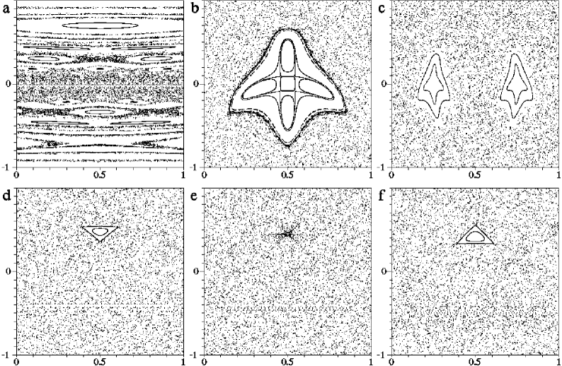
Figure 8: Phase portraits of the billiard in a square. (a) $\mu=30$, (b) $\mu=0.502$, (c) $\mu=\frac{1}{4}$. “Squeeze effect” bifurcation around $\mu=\frac{\sqrt{5}}{2}=1.118\ldots$: (d) $\mu=1.25$, (e) $\mu=1.118$, (f) $\mu=1$.

An interesting resonance phenomenon occurs when $\mu=\frac{\sqrt{5}}{2}$. $S_{4}$ is then a cubic root of ${\mathchoice{\rm 1\mskip-4.0mul}{\rm 1\mskip-4.0mul}{\rm 1\mskip-4.5mul}{\rm 1\mskip-5.0mul}}$, and type I orbit becomes unstable because of a “squeeze effect” bifurcation ([A1], p.392) with a hyperbolic orbit of period 12 (fig.7e, 8d-f). Numerical simulations show no other stable periodic orbits in this case, leading us to the conjecture that the billiard in a square is ergodic for this particular value of $\mu$. Figure 9 illustrates this phenomenon by showing a numerical estimate of the size of regular components of phase space, which vanishes for $\mu=\frac{\sqrt{5}}{2}\simeq 1.118\ldots$.

Figure 9: Numerically estimated proportion of regular component in phase space for the billiard in a square, as a function of $\mu$. Actually, we show the relative area of phase space not occupied by one chaotic orbit, with a precision of $4\cdot 10^{-6}$.

There are no orbits of period 4 when $\mu<\frac{1}{\sqrt{8}}$. However, stable orbits of higher period exist for arbitrarily high values of the magnetic field. Figure 7f shows a symmetric trajectory of period 8, doing 2 bounces on each side of the square. We can construct similar trajectories of period $4k$, $k\geq 1$, reflected $k$ times on each side. Detailed calculations (see appendix E) show that such orbits are stable for almost all $\mu$ in some interval containing $\frac{1}{2k}$, but these intervals do not overlap when $k>2$, leading us to the assumption that mixed and ergodic behaviour alternate for decreasing $\mu$.

6.2 Boundaries with negative curvature

In Sinai billiards, whose boundaries have negative curvature, it is known that all periodic orbits are unstable in zero field (as is suggested by the fact that $\mathchoice{\mbox{$\displaystyle\rm Tr$}}{\mbox{$\textstyle\rm Tr$}}{\mbox{$\scriptstyle\rm Tr$}}{\mbox{$\scriptscriptstyle\rm Tr$}}(DT)\leq-2$ if we put $\chi=0$ in (3)). This is no longer true in non-zero field, because the curved trajectories, although locally dispersed, may converge again.

Figure 10: The billiard outside two circles: (a) chaotic trajectory, (b) one of the few stable trajectories.

Let us first consider billiards outside smooth convex boundaries with extremal radii of curvature $\rho_{\mathchoice{\mbox{$\displaystyle\rm min$}}{\mbox{$\textstyle\rm min$}}{\mbox{$\scriptstyle\rm min$}}{\mbox{$\scriptscriptstyle\rm min$}}}$ and $\rho_{\mathchoice{\mbox{$\displaystyle\rm max$}}{\mbox{$\textstyle\rm max$}}{\mbox{$\scriptstyle\rm max$}}{\mbox{$\scriptscriptstyle\rm max$}}}$. If we fix a trajectory of the outside billiard, and complete every arc of trajectory to a full circle, we obtain its “dual trajectory” as the set of all complementary arcs. If the dual trajectory never crosses the boundary, then it corresponds to a real trajectory of the inside billiard, since the law of specular reflection is satisfied by construction. A sufficient condition for this to be true is that any circle of radius $\mu$ can intersect the boundary at most twice. In this section, let us call this the “$\mu$-intersection property”. This property is actually granted in two cases: in strong field $\mu\leq\rho_{\mathchoice{\mbox{$\displaystyle\rm min$}}{\mbox{$\textstyle\rm min$}}{\mbox{$\scriptstyle\rm min$}}{\mbox{$\scriptscriptstyle\rm min$}}}$ (as we prove in lemma 3 of appendix D), and in weak field $\mu\geq\rho_{\mathchoice{\mbox{$\displaystyle\rm max$}}{\mbox{$\textstyle\rm max$}}{\mbox{$\scriptstyle\rm max$}}{\mbox{$\scriptscriptstyle\rm max$}}}$ (as can be proven in a similar way). In these cases, to any orbit $(\ldots(s_{-1},u_{-1}),(s_{0},u_{0}),(s_{1},u_{1})\ldots)$ of the outside billiard, corresponds the orbit $(\ldots(-s_{1},-u_{1}),(-s_{0},-u_{0}),(-s_{-1},-u_{-1})\ldots)$ of the inside billiard, and reciprocally. Thus, the billiards inside and outside the boundary are perfectly equivalent, so that we can apply our results of section 5 on existence of invariant curves and adiabatic invariants (theorem 1, proposition 3 and the corollary of theorem 2). In particular, the billiard outside a circle is integrable.

For intermediate values of the magnetic field $(\rho_{\mathchoice{\mbox{$\displaystyle\rm min$}}{\mbox{$\textstyle\rm min$}}{\mbox{$\scriptstyle\rm min$}}{\mbox{$\scriptscriptstyle\rm min$}}}<\mu<\rho_{\mathchoice{\mbox{$\displaystyle\rm max$}}{\mbox{$\textstyle\rm max$}}{\mbox{$\scriptstyle\rm max$}}{\mbox{$\scriptscriptstyle\rm max$}}})$, the dual of any outside trajectory will not necessarily be an inside trajectory. However, the equivalence is true for some special trajectories, namely those which are sufficiently close to $u=+1$ for the inside billiard (and remain so because of theorem 1).

Consequently, we predict that if we compare the phase portraits of the billiards inside and outside a given smooth convex curve, they will be the same (up to an inversion) for $\mu\leq\rho_{\mathchoice{\mbox{$\displaystyle\rm min$}}{\mbox{$\textstyle\rm min$}}{\mbox{$\scriptstyle\rm min$}}{\mbox{$\scriptscriptstyle\rm min$}}}$ and $\mu\geq\rho_{\mathchoice{\mbox{$\displaystyle\rm max$}}{\mbox{$\textstyle\rm max$}}{\mbox{$\scriptstyle\rm max$}}{\mbox{$\scriptscriptstyle\rm max$}}}$. When $\rho_{\mathchoice{\mbox{$\displaystyle\rm min$}}{\mbox{$\textstyle\rm min$}}{\mbox{$\scriptstyle\rm min$}}{\mbox{$\scriptscriptstyle\rm min$}}}<\mu<\rho_{\mathchoice{\mbox{$\displaystyle\rm max$}}{\mbox{$\textstyle\rm max$}}{\mbox{$\scriptstyle\rm max$}}{\mbox{$\scriptscriptstyle\rm max$}}}$, the region $u\sim 1$ of the interior portrait will be the same as the region $u\sim-1$ of the exterior portrait, but other parts of them will be different.

Let us consider next the case where the boundary $\partial Q$ has both convex and concave parts, but a bounded curvature: $\left|\kappa(s)\right|\leq\kappa_{0}=\frac{1}{\rho_{\mathchoice{\mbox{$\displaystyle\rm min$}}{\mbox{$\textstyle\rm min$}}{\mbox{$\scriptstyle\rm min$}}{\mbox{$\scriptscriptstyle\rm min$}}}}\forall s$. We can argue by the means of geometrical properties that such a billiard must possess invariant tori and adiabatic invariants in sufficiently strong magnetic field, if $\partial Q$ is smooth enough. It should be clear that the interior of the domain has to be connected, since otherwise we would have several independent billiards. We can thus define $r^{*}$ such that the $\mu$-intersection property is satisfied for $\mu\leq r^{*}$ . This radius has to be positive but can be arbitrarily small (consider billiards shaped like sand-glasses or peanuts).

In section 5.2, we already mentioned that the expression (33) of the bouncing map near $\theta=\pi$ can still be valid if $\mu<\rho_{\mathchoice{\mbox{$\displaystyle\rm min$}}{\mbox{$\textstyle\rm min$}}{\mbox{$\scriptstyle\rm min$}}{\mbox{$\scriptscriptstyle\rm min$}}}(1-\varepsilon)$, namely if $\theta$ is sufficiently close to $\pi$ that the trajectory remains within a distance $2r^{*}$ of the boundary. Thus, invariant curves still exist near $\theta=\pi$. Furthermore, we note that the only point in the proof of proposition 3 where we use the convexity of the boundary is to show the $\mu$-intersection property. This is actually satisfied for $\mu\leq r^{*}$, so that we conclude that proposition 3 and its consequences on adiabatic invariants remain true in the present case, for sufficiently small $\mu$.

Finally, we also studied the billiard outside 2 circles of radius 1, centered at $(0,\pm\lambda)$ (fig.10). If $\lambda>1$, it is important to note that $M_{1}$ defined in section 2 is not the only integrable component of phase space. Indeed, trajectories with $u>u^{*}=\min\left\{1,2\lambda-1-\frac{2\lambda(\lambda-1)}{\mu}\right\}$ always touch the same circle, so that $u$ is a constant of motion. In particular, when $\mu<\lambda-1$, the billiard is integrable. When $\mu>\lambda-1$, the map is discontinuous whenever trajectories become tangent to the boundary, and numerical simulations show that the component of phase space $u<u^{*}$ is almost filled with a stochastic sea with positive Liapunov exponents. However, one can find stable periodic orbits for particular values of the parameters (see appendix F), so that the billiard is not always ergodic.

7 Proof of the adiabatic theorem for maps

7.1 Construction of the change of variables

The change of variables is constructed as the composition of several elementary substitutions, that each increase by one the order of the terms containing the phase. The number of these substitutions is $k$ if the map is $C^{k}$ and of order $\left[1/\mu\right]$ if the map is analytic.

We assume by induction that after $N$ steps, the map reads

$$\varphi_{1} = \varphi_{0}+\mu c(I_{0})\left[\Omega_{N}(I_{0},\mu)+\mu^{N+1}\alpha_{N}(\varphi_{0},I_{0},\mu)\right]$$

$$I_{1} = I_{0}+\mu c(I_{0})^{2}\left[\mu\Theta_{N}(I_{0},\mu)+\mu^{N+1}\beta_{N}(\varphi_{0},I_{0},\mu)\right],$$ (52)

where we write $(\varphi,I)=(\varphi^{(N)},I^{(N)})$ for brevity, and $\Omega_{N}(I,\mu)=\Omega_{0}+\mu\bar{\Omega}_{N}(I,\mu)$. We can assume that $<\alpha_{N}>=<\beta_{N}>=0$, where $<F>=\int_{0}^{1}Fd\varphi$ denotes the average of $F$.

The change of variables $(\varphi,I)\mapsto(\psi,J)=(\varphi^{(N+1)},I^{(N+1)})$ is defined by

$$\psi = \varphi+\mu^{N+1}f(\varphi,I,\mu)$$

$$J = I+\mu^{N+1}c(I)g(\varphi,I,\mu),$$ (53)

where

$$g(\varphi,I,\mu) = \int_{0}^{\varphi}-\frac{1}{\Omega_{0}}\beta_{N}(\varphi^{\prime},I,\mu)d\varphi^{\prime},$$

$$g_{0}(\varphi,I,\mu) = g(\varphi,I,\mu)-<g>(I,\mu),$$

$$f(\varphi,I,\mu) = \int_{0}^{\varphi}\left[c^{\prime}(I)g_{0}(\varphi^{\prime},I,\mu)-\frac{1}{\Omega_{0}}\alpha_{N}(\varphi^{\prime},I,\mu)\right]d\varphi^{\prime}.$$ (54)

We will use the following properties:

1. If $F(\varphi)\in C^{1}$, then

   $$\int_{\varphi_{0}}^{\varphi_{1}}F(\varphi)d\varphi = \mu c(I_{0})\left[\Omega_{N}(I_{0},\mu)F(\varphi_{0})+\mu r_{1}(\varphi_{0},I_{0},\mu)\right]$$ (55)

   $$= \mu c(I_{0})\left[\Omega_{0}F(\varphi_{0})+\mu r_{2}(\varphi_{0},I_{0},\mu)\right].$$

   Indeed, carrying out the change of variables $\varphi=\varphi_{0}+\mu c(I_{0})x$, one obtains

   $$\int_{\varphi_{0}}^{\varphi_{1}}F(\varphi)d\varphi=\mu c(I_{0})\left[\int_{0}^{\Omega_{N}}F(\varphi_{0})dx+\mu c(I_{0})\int_{0}^{\Omega_{N}}F^{\prime}xdx+\int_{\Omega_{N}}^{\Omega_{N}+\mu^{N+1}\alpha_{N}}Fdx\right].$$

2. If $F(I)\in C^{1}$, then

   $$F(I_{0})=F(J_{0})+\mu^{N+1}c(I_{0})r_{3}(\varphi_{0},I_{0},\mu),$$ (56)

   where $r_{3}=-g(\varphi_{0},I_{0},\mu)F^{\prime}(I)$. In particular, $c(I_{0})=c(J_{0})R_{0}(\varphi_{0},I_{0},\mu)$, where $R_{0}=\left[1-\mu^{N+1}gc^{\prime}\right]^{-1}$.

Substituting (52) in (53), we get

$$J_{1}-J_{0} = \mu^{N+1}\left[c(I_{1})g(\varphi_{1},I_{1},\mu)-c(I_{0})g(\varphi_{0},I_{0},\mu)\right]+$$ (57)

$$+\mu^{2}c(I_{0})^{2}\left[\Theta_{N}(I_{0},\mu)+\mu^{N}\beta_{N}(\varphi_{0},I_{0},\mu)\right].$$

Now, using the above properties, we obtain

$$c(I_{1})g(\varphi_{1},I_{1},\mu)-c(I_{0})g(\varphi_{1},I_{0},\mu) = (I_{1}-I_{0})\partial_{I}\left[c(I)g(\varphi_{1},I,\mu)\right]$$

$$= \mu^{2}c(I_{0})^{2}R_{1}(\varphi_{0},I_{0},\mu),$$

$$c(I_{0})g(\varphi_{1},I_{0},\mu)-c(I_{0})g(\varphi_{0},I_{0},\mu) = -\frac{1}{\Omega_{0}}c(I_{0})\int_{\varphi_{0}}^{\varphi_{1}}\beta_{N}(\varphi,I_{0},\mu)d\varphi$$

$$= -\mu c(I_{0})^{2}\beta_{N}(\varphi_{0},I_{0},\mu)+$$

$$+\mu^{2}c(I_{0})^{2}R_{2}(\varphi_{0},I_{0},\mu),$$

$$c(I_{0})\Theta_{N}(I_{0},\mu)-c(J_{0})\Theta_{N}(J_{0},\mu) = \mu^{N+1}c(I_{0})R_{3}(\varphi_{0},I_{0},\mu),$$

$$c(I_{0})-c(J_{0}) = \mu^{N+1}c(I_{0})r_{4}(\varphi_{0},I_{0},\mu).$$ (58)

Replacing this in (57), we finally get

$$J_{1}=J_{0}+\mu^{2}c(J_{0})^{2}\Theta_{N}(J_{0},\mu)+\mu^{N+3}c(J_{0})^{2}\tilde{\beta}_{N+1}(\varphi_{0},I_{0},\mu),$$ (59)

where $\tilde{\beta}_{N+1}=R_{0}^{2}(R_{1}+R_{2}+R_{3})+R_{0}R_{4}$ and $R_{4}=\Theta_{N}r_{4}$. The final step is to write $\tilde{\beta}_{N+1}(\varphi_{0},I_{0},\mu)=\hat{\beta}_{N+1}(\psi_{0},J_{0},\mu)$, which can be done for small enough $\mu$, as we shall check later, and $\Theta_{N+1}=\Theta_{N}+\mu^{N+1}<\hat{\beta}_{N+1}>,\beta_{N+1}=\hat{\beta}_{N+1}-<\hat{\beta}_{N+1}>$.

Proceeding in a similar way for $\psi$, we obtain

$$\psi_{1}-\psi_{0} = \mu c(I_{0})\Omega_{N}(I_{0},\mu)\left[1+\mu^{N+1}c^{\prime}(I_{0})g_{0}(\varphi_{0},I_{0},\mu)\right]+\mu^{N+3}c(I_{0})R_{5}$$

$$c(I_{0})\Omega_{N}(I_{0},\mu) = c(J_{0})\Omega_{N}(J_{0},\mu)+\mu^{N+1}c(I_{0})\left[-\Omega_{N}(I_{0},\mu)c^{\prime}(I_{0})g(\varphi_{0},I_{0},\mu)+\mu R_{6}\right]$$

$$c(I_{0})c^{\prime}(I_{0})\Omega_{N}(I_{0},\mu)<g>(I_{0},\mu)=c(J_{0})c^{\prime}(J_{0})\Omega_{N}(J_{0},\mu)<g>(J_{0},\mu)-\mu c(I_{0})R_{7},$$

so that

$$\psi_{1}=\psi_{0}+\mu c(J_{0})\hat{\Omega}_{N}(J_{0},\mu)+\mu^{N+3}c(J_{0})\tilde{\alpha}_{N+1}(\varphi_{0},I_{0},\mu).$$ (60)

where $\tilde{\alpha}_{N+1}=R_{0}(R_{5}+R_{6}+R_{7})$ and $\hat{\Omega}_{N}=\Omega_{N}(1-\mu^{N+1}c^{\prime}<g>)$. Finally, we proceed in the same way as for $\beta$ in order to define $\Omega_{N+1},\alpha_{N+1}$.

7.2 Bounds and domains of analyticity

In the case where the map is analytic, we define

$$\Gamma(D)=\left\{(\varphi,I)\mid\left|\mathchoice{\mbox{$\displaystyle\rm Im$}}{\mbox{$\textstyle\rm Im$}}{\mbox{$\scriptstyle\rm Im$}}{\mbox{$\scriptscriptstyle\rm Im$}}\varphi\right|,\left|\mathchoice{\mbox{$\displaystyle\rm Im$}}{\mbox{$\textstyle\rm Im$}}{\mbox{$\scriptstyle\rm Im$}}{\mbox{$\scriptscriptstyle\rm Im$}}I\right|<D,-D<\mathchoice{\mbox{$\displaystyle\rm Re$}}{\mbox{$\textstyle\rm Re$}}{\mbox{$\scriptstyle\rm Re$}}{\mbox{$\scriptscriptstyle\rm Re$}}I<1+D\right\}.$$ (61)

We assume that for $(\varphi,I)\in\Gamma(D_{N})$ and $\left|\mu\right|<\mu_{0}$, (52) is analytic and satisfies the bounds $\left|\alpha_{N}\right|,\left|\beta_{N}\right|\leq M_{N}$, $\left|\bar{\Omega}_{N}\right|,\left|\Theta_{N}\right|\leq W_{N}$. We introduce numbers $D_{N}^{\prime\prime}<D_{N}^{\prime}<D_{N}$, such that $(\varphi_{0},I_{0})\in\Gamma(D_{N}^{\prime\prime})$ implies $(\varphi_{1},I_{1}),(\psi_{0},J_{0})\in\Gamma(D_{N}^{\prime})$. Thus, $D_{N}^{\prime\prime}$ has to satisfy the condition

$$D_{N}^{\prime\prime}\leq D_{N}^{\prime}-k_{0}\max\left\{\mu_{0}+\mu_{0}^{2}W_{N}+\mu_{0}^{N+2}M_{N},\mu_{0}^{N+1}M_{N}\right\}.$$ (62)

From now on, the numbers $k_{i},\lambda_{i},c_{i}$ will designate constants which are uniform in $N$ and $\mu$. Using Cauchy’s inequality to bound the derivatives appearing in the expressions of the $R_{i}$, we obtain that for $(\varphi_{0},I_{0})\in\Gamma(D_{N}^{\prime\prime})$, $\left|R_{i}\right|\leq K_{i}$, where

$$K_{0} = \frac{1}{1-\mu_{0}^{N+1}\lambda_{0}M_{N}}$$

$$K_{1} = \lambda_{1}\left[W_{N}+\mu_{0}^{N}M_{N}\right]\frac{M_{N}}{D_{N}-D_{N}^{\prime}}$$

$$K_{2} = \lambda_{2}\left[W_{N}+\mu_{0}^{N}M_{N}+\frac{1}{D_{N}-D_{N}^{\prime}}\right]M_{N}$$

$$K_{3} = \lambda_{3}\frac{M_{N}W_{N}}{D_{N}-D_{N}^{\prime}}$$

$$K_{4} = \lambda_{4}M_{N}W_{N}$$

$$K_{5} = \lambda_{5}\left[\frac{W_{N}+\mu_{0}^{N}M_{N}}{D_{N}-D_{N}^{\prime}}+\mu_{0}^{N}M_{N}+\frac{1+\mu_{0}W_{N}}{D_{N}-D_{N}^{\prime}}\right]M_{N}$$

$$K_{6} = \lambda_{6}\left[1+\mu_{0}^{N}M_{N}\right]\frac{M_{N}W_{N}}{D_{N}-D_{N}^{\prime}}$$

$$K_{7} = \lambda_{7}\mu_{0}^{N}M_{N}\frac{M_{N}W_{N}}{D_{N}-D_{N}^{\prime}},$$ (63)

and the new bounds have to satisfy

$$M_{N+1} \geq c_{1}\max\left\{K_{0}^{2}\sum_{i=1}^{3}K_{i}+K_{0}K_{4},K_{0}\sum_{i=5}^{7}K_{i}\right\}$$

$$W_{N+1} \geq W_{N}+c_{2}\mu_{0}^{N+1}(W_{N}M_{N}+M_{N+1}).$$ (64)

Finally, we have to consider the effect of the change of variables on the domain of analyticity.

Lemma 1 If $F(\varphi,I,\mu)$ is analytic for $(\varphi,I)\in\Gamma(D)$, then $\bar{F}(\psi,J,\mu)=F(\varphi,I,\mu)$ is analytic for $(\psi,J)\in\Gamma(D-4c_{0}\mu_{0}^{N+1}M_{N})$.

Proof: Write $x=(\varphi,I),y=(\psi,J)$. From (53), we have $y=x+G(x)$, with $\left|G_{i}(x)\right|\leq c_{0}\mu_{0}^{N+1}M_{N}$. If $\Phi(x,y)=x+G(x)-y$ and $\left|\partial_{i}G_{j}\right|\leq\varepsilon$, then $\det(\partial_{x}\Phi)\geq 1-2\varepsilon-2\varepsilon^{2}$. If $y\in\Gamma(D-4c_{0}\mu_{0}^{N+1}M_{N})$, then $x\in\Gamma(D-3c_{0}\mu_{0}^{N+1}M_{N})$, and Cauchy’s inequality implies $\varepsilon<1/3$, so that $\det(\partial_{x}\Phi)>0$. The implicit function theorem implies that we can write $x=\xi(y)$ where $\xi$ is analytic, and so is $\bar{F}(y,\mu)=F(\xi(y),\mu)$.     $\sqcap$$\sqcup$

Hence, we must take

$$D_{N+1}\leq D_{N}^{\prime\prime}-4c_{0}\mu_{0}^{N+1}M_{N}.$$ (65)

7.3 Evolution of the bounds with $N$

We now choose domains of the form $D_{N}=D_{0}-Nd\mu_{0}$, $D_{N}^{\prime}=D_{N}-d^{\prime}\mu_{0}$, $d^{\prime}<d$. We wish to show by induction that for a suitable choice of $d$ and $d^{\prime}$ and $\mu_{0}$ small enough,

$$M_{N} = \frac{M_{0}}{(2\mu_{0})^{N}},$$ (66)

$$W_{N} = W_{0}+c_{3}\left(1-\frac{1}{2^{N}}\right).$$ (67)

Replacing this in (63), we get $K_{0}\leq\left[1-\mu_{0}\lambda_{0}M_{0}\right]^{-1}\leq 2$ if $\mu_{0}\leq\left[2\lambda_{0}M_{0}\right]^{-1}$, and $K_{i}\leq k_{i}M_{N}/d^{\prime}\mu_{0},i=1\ldots 7$. Thus, we can take

$$M_{N+1}=c_{1}m\frac{M_{N}}{d^{\prime}\mu_{0}}=\frac{M_{N}}{2\mu_{0}}$$ (68)

where $d^{\prime}=2c_{1}m$ and $m=\max\left\{4\sum_{i=1}^{3}k_{i}+2k_{4},2\sum_{i=5}^{7}k_{i}\right\}$.

To prove (67), we take $c_{3}=W_{0}+c_{2}M_{0}$, $\overline{W}=W_{0}+c_{3}$ and $\mu_{0}\leq W_{0}\left[2c_{2}M_{0}\overline{W}\right]^{-1}$, so that

$$c_{2}\mu_{0}^{N+1}(W_{N}M_{N}+M_{N+1})\leq\frac{c_{2}M_{0}}{2^{N}}\left[\mu_{0}\overline{W}+\frac{1}{2}\right]\leq\frac{1}{2^{N}}\left[\frac{W_{0}}{2}+\frac{c_{2}M_{0}}{2}\right]=\frac{c_{3}}{2^{N+1}}.$$

Finally, it is easy to check that the conditions (62) and (65) are satisfied if we take $d=d^{\prime}+4c_{0}M_{0}+k_{0}\max\left\{1+\mu^{*}(\overline{W}+M_{0}),M_{0}\right\}$.

The last step in order to prove (46) is to take

$$N=N(\mu_{0})=\left[\frac{D_{0}}{d\mu_{0}}\right].$$ (69)

In this way, $W_{N(\mu_{0})}$ is bounded, $D_{N(\mu_{0})}$ is still positive so that $\Gamma(M_{N(\mu_{0})})$ is not empty, and the terms containing the phase are bounded by

$$\mu_{0}^{N(\mu_{0})}M_{N(\mu_{0})}=\frac{M_{0}}{2^{N(\mu_{0})}}=M_{0}\mathchoice{\mbox{$\displaystyle\rm e$}}{\mbox{$\textstyle\rm e$}}{\mbox{$\scriptstyle\rm e$}}{\mbox{$\scriptscriptstyle\rm e$}}^{-\ln 2\left[D_{0}/d\mu_{0}\right]}=M_{0}\mathchoice{\mbox{$\displaystyle\rm e$}}{\mbox{$\textstyle\rm e$}}{\mbox{$\scriptstyle\rm e$}}{\mbox{$\scriptscriptstyle\rm e$}}^{-1/C\mu_{0}}.$$ (70)

Finally, we also see that the terms defining the successive changes of variables, i.e. $\mu_{0}^{N+1}f_{N}$, where $f_{N}\sim M_{N}$, add up to a geometrical series converging towards a term of order $\mu_{0}$.

7.4 Conservative case

It is easy to check that if (45) preserves the measure $c(I)\rho(\varphi,I,\mu)d\varphi dI$, $\rho(\varphi,I,0)=1$, then (52) preserves the measure $c(I)\rho_{N}(\varphi,I,\mu)d\varphi dI$, $\rho_{N}(\varphi,I,0)=1$. As long as (52) is $C^{1}$ and $c\in C^{2}$, we can apply the

Lemma 2 If (52) preserves the measure $c(I)\rho d\varphi dI$, then $\Theta_{N}(I_{0},\mu)=O(\mu^{N+1})$ and $\partial_{\varphi}\rho=O(\mu^{N+1})$.

Proof: We assume by induction that $\Theta_{N}c(I)=\mu^{p}\overline{\Theta}_{N}$ and $\rho(\varphi,I,\mu)=\rho_{0}(I,\mu)+\mu^{p+1}\rho_{1}(\varphi,I,\mu)$, which is clearly true for $p=0$. We have

$$\frac{c(I_{1})\rho(\varphi_{1},I_{1},\mu)}{c(I_{0})\rho(\varphi_{0},I_{0},\mu)} = \det\left(\begin{array}[]{cc}1+\mu^{N+2}c(I_{0})\partial_{\varphi}\alpha_{N}&O(\mu)\\ O(\mu^{N+2})&1+\mu^{p+2}\partial_{I}(c\overline{\Theta}_{N})+\mu^{N+2}\partial_{I}(c^{2}\beta_{N})\end{array}\right)$$ (74)

$$= 1+\mu^{p+2}\partial_{I}\left[c(I_{0})\overline{\Theta}_{N}(I_{0},0)\right]+\mu^{N+2}\left(c\partial_{\varphi}\alpha_{N}+\partial_{I}\left[c^{2}\beta_{N}\right]\right)+$$

$$+O(\mu^{p+3})+O(\mu^{N+3}).$$

On the other hand, making expansions, we obtain

$$\frac{c(I_{1})\rho(\varphi_{1},I_{1},\mu)}{c(I_{0})\rho(\varphi_{0},I_{0},\mu)} = 1+\mu^{p+2}\left[c(I_{0})\Omega_{0}\partial_{\varphi}\rho_{1}(\varphi_{0},I_{0},0)+c^{\prime}(I_{0})\overline{\Theta}_{N}(I_{0},0)\right]+$$ (75)

$$+\mu^{N+2}c(I_{0})c^{\prime}(I_{0})\beta_{N}(\varphi_{0},I_{0},0)+O(\mu^{p+3})+O(\mu^{N+3}).$$

Comparing (74) and (75), we obtain for $p<N$

$$\Omega_{0}\partial_{\varphi}\rho_{1}(\varphi_{0},I_{0},0)=\partial_{I}\overline{\Theta}_{N}(I_{0},0).$$ (76)

The left-hand side is a periodic function of $\varphi$ with average $0$. Hence, the right-hand side must vanish. This implies $\partial_{\varphi}\rho_{1}=0$ and $\overline{\Theta}_{N}=\mbox{const}$. But this constant must be zero since $\overline{\Theta}_{N}$ is divisible by $c(I)$. This proves $p=N$ by induction. For $p=N$, one obtains again that $\partial_{I}\overline{\Theta}_{N}$ is a periodic function of $\varphi$ with average $0$, which proves the lemma.     $\sqcap$$\sqcup$

In the $C^{k}$ case, we first do $k-1$ changes of variables, so that the map takes the form (52) with $N=k-1$ and is $C^{1}$. Then we can apply the above lemma, and finally we do the change of variables (53) with $N=k$, which proves (49).

In the analytic case, after $N(\mu_{0})$ changes of variables, the lemma implies that we can write $\Theta_{N}(I,\mu)=\mu^{N}\hat{\Theta}_{N}(I,\mu)$, and Cauchy’s inequality gives

$$\left|\hat{\Theta}_{N}(I,\mu)\right|\leq\frac{\overline{W}}{(\mu_{0}-\left|\mu\right|)^{N}}.$$ (77)

For $\mu_{1}=\mu_{0}/3$, we have

$$\left|\mu_{1}^{N}\hat{\Theta}_{N}\right|\leq\frac{\overline{W}}{2^{N}},\;\;\;\left|\mu_{1}^{N}\beta_{N}\right|\leq\frac{M_{0}}{6^{N}},$$ (78)

which proves (47).     $\sqcap$$\sqcup$

8 Conclusion

In this work on classical billiards in plane domains, we found that some properties of bouncing maps, which are known in the Euclidean case, can be generalized to the situation where a magnetic field is applied perpendicularly to the plane. Exact expressions for the Jacobian matrix and a generating function help to find periodic orbits, analyze their stability and compute bifurcation values. Perturbative calculations are improved.

Some aspects of the behaviour of billiards in convex domains are well understood: if the boundary is sufficiently smooth, existence of whispering gallery modes prevents ergodicity, and when the magnetic field $B$ goes to infinity, the bouncing map behaves like a perturbed integrable map. We were able to construct quasi-invariants, which are conserved for a time of order $B^{k-3}$ if the boundary is $C^{k}$, and of order $\mathchoice{\mbox{$\displaystyle\rm e$}}{\mbox{$\textstyle\rm e$}}{\mbox{$\scriptstyle\rm e$}}{\mbox{$\scriptscriptstyle\rm e$}}^{B}$ when the boundary is analytic. Some of these properties remain valid for a more general class of billiards, the boundary of which is not convex, but has a bounded curvature.

Chaotic behaviour seems to be created by two different mechanisms: non-linearity (responsible for instance of chaotic components near separatrices) and singularities (due to non-smooth boundaries or discontinuities by tangency). Non-linearity alone is not sufficient to make a magnetic billiard ergodic, since we showed that there always exist invariant curves if the boundary is $C^{6}$ and tangencies are impossible. This implies in particular that billiards with boundaries of negative curvature are not necessarily very chaotic. In any case where the billiard is of the mixed type, the really challenging open problem remains to prove the existence of a chaotic component of positive measure.

Finally, we discussed two examples of billiards fulfilling necessary conditions for ergodicity (i.e. their bouncing maps have singularities). Our study of symmetric periodic orbits in the square lead us to the conjecture that ergodic and mixed dynamics alternate when the magnetic field increases. However, only the first value of supposed ergodicity, $\mu=\frac{\sqrt{5}}{2}$, lies in the region $\mu>\frac{1}{2}$, where no trivially integrable component of phase space exists. The scattering billiard outside two circles shows strongly chaotic dynamics, but still possesses elliptic orbits for some values of the parameters.

Appendix A Proof of proposition 1

We consider the arc of trajectory in figure 2. If

$$\alpha=\arg\left[\left(X(s_{1})-X(s_{0})\right)+\mathchoice{\mbox{$\displaystyle\rm i$}}{\mbox{$\textstyle\rm i$}}{\mbox{$\scriptstyle\rm i$}}{\mbox{$\scriptscriptstyle\rm i$}}\left(Y(s_{1})-Y(s_{0})\right)\right]$$ (79)

is the angle between the $x$-axis and $P_{0}P_{1}$, then we have

$$\theta_{0} = \alpha-\tau_{0}-\chi,$$

$$\theta_{1} = \tau_{1}-\alpha-\chi.$$ (80)

Now, using (6) and $\ell^{2}=(X(s_{1})-X(s_{0}))^{2}+(Y(s_{1})-Y(s_{0}))^{2}$, we find

$$\frac{\partial\alpha}{\partial s_{0}} = \frac{1}{\ell^{2}}\left[\left(Y(s_{1})-Y(s_{0})\right)X^{\prime}(s_{0})-\left(X(s_{1})-X(s_{0})\right)Y^{\prime}(s_{0})\right]$$

$$= \frac{\sin\alpha\cos\tau_{0}-\cos\alpha\sin\tau_{0}}{\ell}=\frac{\sin(\theta_{0}+\chi)}{\ell},$$

$$\frac{\partial\tau_{0}}{\partial s_{0}} = \kappa(s_{0})=\kappa_{0},$$

$$\frac{\partial\chi}{\partial s_{0}} = \frac{1}{\cos\chi}\frac{1}{2\mu}\frac{\partial\ell}{\partial s_{0}}=-\frac{\cos(\theta_{0}+\chi)}{2\mu\cos\chi}=-\frac{\cos(\theta_{0}+\chi)\sin\chi}{\ell\cos\chi},$$ (81)

where the last equality comes from the zero-field generating property of $\ell$:

$$\frac{\partial\ell}{\partial s_{0}} = \frac{1}{\ell}\left[-X^{\prime}(s_{0})\left(X(s_{1})-X(s_{0})\right)-Y^{\prime}(s_{0})\left(Y(s_{1})-Y(s_{0})\right)\right]$$ (82)

$$= -\cos\alpha\cos\tau_{0}-\sin\alpha\sin\tau_{0}=-\cos(\theta_{0}+\chi).$$

Collecting terms, we get

$$\frac{\partial\theta_{0}}{\partial s_{0}}=\frac{\sin(\theta_{0}+2\chi)}{\ell\cos\chi}-\kappa_{0},\phantom{MM}\frac{\partial\theta_{1}}{\partial s_{0}}=-\frac{\sin\theta_{0}}{\ell\cos\chi}.$$ (83)

Similarly, we find

$$\frac{\partial\theta_{0}}{\partial s_{1}}=\frac{\sin\theta_{1}}{\ell\cos\chi},\phantom{MM}\frac{\partial\theta_{1}}{\partial s_{1}}=-\frac{\sin(\theta_{1}+2\chi)}{\ell\cos\chi}+\kappa_{1}.$$ (84)

These quantities give $d\theta_{0}$ and $d\theta_{1}$ in function of $ds_{0}$ and $ds_{1}$. Solving a linear system, we can express $ds_{1}$ and $d\theta_{1}$ as functions of $ds_{0}$ and $d\theta_{0}$. Finally, using $du=\sin\theta d\theta$, we obtain the equations (3).     $\sqcap$$\sqcup$

Appendix B Proof of proposition 2

Taking the derivative of (14) and using (6), we get

$$\frac{\partial B_{\mu}}{\partial\ell}=\sqrt{1-\frac{\ell^{2}}{4\mu^{2}}}=\cos\chi.$$ (85)

From simple geometry, we obtain

$$\frac{\partial A}{\partial s_{0}}=-\frac{1}{2}\ell\sin(\theta_{0}+\chi),$$ (86)

so that the derivative of (13) is

$$\frac{\partial G}{\partial s_{0}}=\frac{1}{\mu}\frac{\partial A}{\partial s_{0}}+\frac{\partial B_{\mu}}{\partial\ell}\frac{\partial\ell}{\partial s_{0}}=-\sin\chi\sin(\theta_{0}+\chi)-\cos\chi\cos(\theta_{0}+\chi)=u_{0},$$ (87)

where we have used (82) and (6) again. We proceed in a similar way for $s_{1}$.     $\sqcap$$\sqcup$

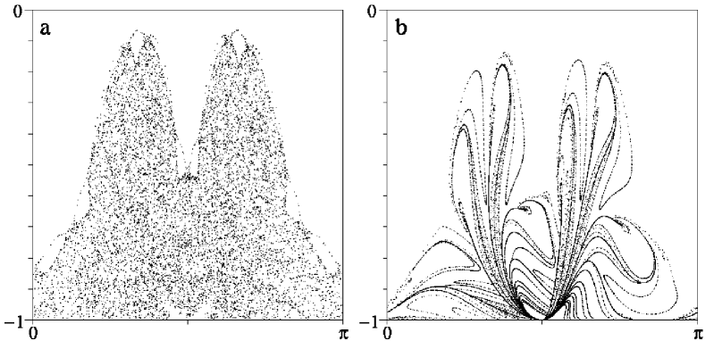
Figure 11: Behaviour near $u=-1$ of the billiard in an ellipse when $\rho_{\mathchoice{\mbox{$\displaystyle\rm min$}}{\mbox{$\textstyle\rm min$}}{\mbox{$\scriptstyle\rm min$}}{\mbox{$\scriptscriptstyle\rm min$}}}<\mu<\rho_{\mathchoice{\mbox{$\displaystyle\rm max$}}{\mbox{$\textstyle\rm max$}}{\mbox{$\scriptstyle\rm max$}}{\mbox{$\scriptscriptstyle\rm max$}}}$ ($\mu=1$, $\lambda=2$): (a) chaotic orbit near $u=-1$, (b) the preimages ${\cal D}_{n}$, $n=1\ldots 15$ of the line $u=-1$.

Appendix C Discontinuities of the map due to tangencies

The bouncing map is discontinuous either in the corners of the boundary ($s\in E_{1}$), or if the trajectory becomes tangent to the boundary. As can be seen in fig.4b, such a tangency means that there are two arbitrarily close initial conditions $z_{1},z_{2}$ such that $Tz_{2}$ is far away from $Tz_{1}$ but close to $T^{2}z_{1}$. Then there exists a point $z^{*}$ between $z_{1}$ and $z_{2}$ such that $Tz^{*}=(s^{*},-1)$ (or $(s^{*},+1)$ if $\partial Q$ is not convex).

Let ${\cal C}=[0,\left|\partial Q\right|)\times\left\{-1,+1\right\}$. It can be written as the union of 3 disjoint sets:

• the set ${\cal C}_{0}$ of $z\in{\cal C}$ such that $T^{-1}z$ does not exist;

• the set ${\cal C}_{1}$ of $z\in{\cal C}$ such that $T^{-1}z\in{\cal C}$;

• the set ${\cal C}_{2}$ of $z\in{\cal C}$ such that $T^{-1}z\not\in{\cal C}$.

The set ${\cal D}$ of lines of discontinuity of $T$ is $T^{-1}{\cal C}_{2}$.

To construct the sets ${\cal C}_{i}$, we first look for circles of radius $\mu$ which are inscribed in $Q$, i.e. circles contained in $\overline{Q}$ and tangent to $\partial Q$ at two points or more. Let $\widehat{E}$ be the set of abscissas $\widehat{s}_{i}$ of these contact points. Let $\widetilde{E}$ be set of abscissas $\widetilde{s}_{j}$ such that $\left|\rho(\widetilde{s}_{j})\right|=\mu$. Then ${\cal C}_{0}$, ${\cal C}_{1}$ and ${\cal C}_{2}$ are delimited by points with abscissa in $\widehat{E}$, $\widetilde{E}$ and $E_{2}$ (see [RB] for a more geometric interpretation of these sets).

We illustrate this construction in the case of an elliptic boundary (15), using $\varphi$ instead of $s$. Here we take ${\cal C}=[0,\left|\partial Q\right|)\times\left\{-1\right\}$. Inscribed circles exist if $\rho_{\mathchoice{\mbox{$\displaystyle\rm min$}}{\mbox{$\textstyle\rm min$}}{\mbox{$\scriptstyle\rm min$}}{\mbox{$\scriptscriptstyle\rm min$}}}=\lambda^{-1}<\mu\leq 1$, and their contact points are solutions of

$$\sin^{2}\widehat{\varphi}_{i}=\frac{(\lambda\mu)^{2}-1}{\lambda^{2}-1}.$$ (88)

If $\rho_{\mathchoice{\mbox{$\displaystyle\rm min$}}{\mbox{$\textstyle\rm min$}}{\mbox{$\scriptstyle\rm min$}}{\mbox{$\scriptscriptstyle\rm min$}}}=\lambda^{-1}<\mu\leq\rho_{\mathchoice{\mbox{$\displaystyle\rm max$}}{\mbox{$\textstyle\rm max$}}{\mbox{$\scriptstyle\rm max$}}{\mbox{$\scriptscriptstyle\rm max$}}}=\lambda^{2}$, there are points $\widetilde{\varphi}_{j}$, given by

$$\sin^{2}\widetilde{\varphi}_{j}=\frac{(\lambda\mu)^{2/3}-1}{\lambda^{2}-1}.$$ (89)

If they exist, the solutions can be ordered $0\leq\widetilde{\varphi}_{1}\leq\widehat{\varphi}_{1}\leq\widehat{\varphi}_{2}\leq\widetilde{\varphi}_{2}\leq\widetilde{\varphi}_{3}\leq\widehat{\varphi}_{3}\leq\widehat{\varphi}_{4}\leq\widetilde{\varphi}_{4}\leq 2\pi$. They satisfy

$$T^{-1}(\widehat{\varphi}_{i},-1)=(\widehat{\varphi}_{5-i},-1) i=1,2,3,4,$$ for (90)

$$\lim_{\varphi\rightarrow\widetilde{\varphi}_{j}+}T^{-1}(\varphi,-1)=(\widetilde{\varphi}_{j},-1) j=1,3.$$ for (91)

Table 1 shows the resulting subsets of ${\cal C}$. Following ideas in [DR], one can look at the successive preimages ${\cal D}_{n}=T^{-n}{\cal C}_{2}$ of the lines of discontinuity. Numerical simulations show that they densely fill the stochastic layer near $u=-1$ (see fig.11).

Table 1: The sets ${\cal C}_{0}$, ${\cal C}_{1}$ and ${\cal C}_{2}$ for an elliptic boundary.

$\mu\in$	${\cal C}_{0}$	${\cal C}_{1}$	${\cal C}_{2}$
$(0,\rho_{\mathchoice{\mbox{$\displaystyle\rm min$}}{\mbox{$\textstyle\rm min$}}{\mbox{$\scriptstyle\rm min$}}{\mbox{$\scriptscriptstyle\rm min$}}}]$	$\emptyset$	${\cal C}$	$\emptyset$
$(\rho_{\mathchoice{\mbox{$\displaystyle\rm min$}}{\mbox{$\textstyle\rm min$}}{\mbox{$\scriptstyle\rm min$}}{\mbox{$\scriptscriptstyle\rm min$}}},1]$	$(\widetilde{\varphi}_{2},\widetilde{\varphi}_{3}]\cup(\widetilde{\varphi}_{4},\widetilde{\varphi}_{1}]$	$[\widehat{\varphi}_{1},\widehat{\varphi}_{2}]\cup[\widehat{\varphi}_{3},\widehat{\varphi}_{4}]$	$(\widetilde{\varphi}_{1},\widehat{\varphi}_{1})\cup(\widehat{\varphi}_{2},\widetilde{\varphi}_{2}]\cup$
	$\times\left\{-1\right\}$	$\times\left\{-1\right\}$	$(\widetilde{\varphi}_{3},\widehat{\varphi}_{3})\cup(\widehat{\varphi}_{4},\widetilde{\varphi}_{4}]\times\left\{-1\right\}$
$(1,\rho_{\mathchoice{\mbox{$\displaystyle\rm max$}}{\mbox{$\textstyle\rm max$}}{\mbox{$\scriptstyle\rm max$}}{\mbox{$\scriptscriptstyle\rm max$}}})$	$(\widetilde{\varphi}_{2},\widetilde{\varphi}_{3}]\cup(\widetilde{\varphi}_{4},\widetilde{\varphi}_{1}]$	$\emptyset$	$(\widetilde{\varphi}_{1},\widetilde{\varphi}_{2}]\cup(\widetilde{\varphi}_{3},\widetilde{\varphi}_{4}]$
	$\times\left\{-1\right\}$		$\times\left\{-1\right\}$
$[\rho_{\mathchoice{\mbox{$\displaystyle\rm max$}}{\mbox{$\textstyle\rm max$}}{\mbox{$\scriptstyle\rm max$}}{\mbox{$\scriptscriptstyle\rm max$}}},\infty)$	${\cal C}$	$\emptyset$	$\emptyset$

Appendix D Proof of proposition 3

The following geometrical lemma describes some properties of convex plane curves (which seem quite obvious if one draws a picture).

Lemma 3 Let $D$ be a circular segment of angle $2\alpha\in(0,\pi]$ and radius $1$. Let ${\cal C}$ be a strictly convex $C^{2}$ curve with extremities on the vertices $A_{0},B_{0}$ of $D$, and making acute or right angles with the chord $A_{0}B_{0}$ (see fig.12). Then, if the curvature of ${\cal C}$ is everywhere less than $1$, it is entirely contained in $D$ and shorter than $2\alpha$.

Figure 12: Geometry of the circular segment of lemma 3.

Proof: We introduce coordinate axes as in figure 12. For $-\sin\alpha<x<\sin\alpha$, ${\cal C}$ can be described by a function $y(x)$, and the curvature is

$$\kappa(x)=-\frac{y^{\prime\prime}(x)}{(1+y^{\prime}(x))^{3/2}}\in(0,1).$$ (92)

This equation can be integrated between the abscissa $x_{0}$ of the maximum $S_{0}$ and $x$:

$$y^{\prime}(x) = -\frac{k(x)}{\sqrt{1-k(x)^{2}}}$$

$$k(x) = \int_{x_{0}}^{x}\kappa(x_{1})dx_{1},\;\left|k(x)\right|<\left|x-x_{0}\right|.$$ (93)

For $x_{0}-1<x<x_{0}+1$, this implies

$$\left[y(x)-(y(x_{0})-1)\right]^{2}+(x-x_{0})^{2}\geq 1,$$ (94)

and hence ${\cal C}$ lies above the circle of radius 1 tangent to it at its summit $S_{0}$. Now assume by contradiction that ${\cal C}$ lies outside $D$ between two points $P$ and $P^{\prime}$. Let $S$ be the point of ${\cal C}$ furthest away from $PP^{\prime}$. The circle of unit radius tangent to ${\cal C}$ at $S$ cannot intersect $D$ twice between $P$ and $P^{\prime}$, which contradicts (94).

If $P$ and $P^{\prime}$ are two points of ${\cal C}$, we denote by $\overline{PP^{\prime}}$ the length of ${\cal C}$ between these points. If $P(x)=(x,y(x))$, then for $x_{0}-1<x<x_{0}+1$,

$$\overline{S_{0}P(x)}=\int_{x_{0}}^{x}\sqrt{1+y^{\prime}(x_{1})^{2}}dx_{1}\leq\mathchoice{\mbox{$\displaystyle\rm Arcsin$}}{\mbox{$\textstyle\rm Arcsin$}}{\mbox{$\scriptstyle\rm Arcsin$}}{\mbox{$\scriptscriptstyle\rm Arcsin$}}\left|x-x_{0}\right|.$$ (95)

Assume that $x_{0}\leq 0$. Then $\overline{A_{0}A_{1}}\leq\mathchoice{\mbox{$\displaystyle\rm Arcsin$}}{\mbox{$\textstyle\rm Arcsin$}}{\mbox{$\scriptstyle\rm Arcsin$}}{\mbox{$\scriptscriptstyle\rm Arcsin$}}(x_{0}+\sin\alpha)+\mathchoice{\mbox{$\displaystyle\rm Arcsin$}}{\mbox{$\textstyle\rm Arcsin$}}{\mbox{$\scriptstyle\rm Arcsin$}}{\mbox{$\scriptscriptstyle\rm Arcsin$}}(-x_{0})\leq\alpha$ by convexity of $\textstyle\rm Arcsin$. Considering the circular segment of vertices $A_{1}$ and $B_{0}$, one obtains that $\overline{A_{1}B_{0}}$ can be divided into two parts, one of which is bounded by $\frac{\alpha}{2}$. Repeating this procedure, we see that ${\cal C}$ can be divided into pieces whose lengths are bounded by a geometrical series, converging towards $2\alpha$.     $\sqcap$$\sqcup$

Corollary Let ${\cal C}$ be a $C^{2}$ plane convex curve, whose curvature satisfies $0<\frac{1}{\rho_{\mathchoice{\mbox{$\displaystyle\rm max$}}{\mbox{$\textstyle\rm max$}}{\mbox{$\scriptstyle\rm max$}}{\mbox{$\scriptscriptstyle\rm max$}}}}\leq\kappa(s)\leq\frac{1}{\rho_{\mathchoice{\mbox{$\displaystyle\rm min$}}{\mbox{$\textstyle\rm min$}}{\mbox{$\scriptstyle\rm min$}}{\mbox{$\scriptscriptstyle\rm min$}}}}<\infty$. Let $\Gamma$ be a circle of radius $\mu<\rho_{\mathchoice{\mbox{$\displaystyle\rm min$}}{\mbox{$\textstyle\rm min$}}{\mbox{$\scriptstyle\rm min$}}{\mbox{$\scriptscriptstyle\rm min$}}}$. Then

1. $\Gamma$ can be tangent to ${\cal C}$ at one point at most.

2. $\Gamma$ can intersect ${\cal C}$ at two points at most.

   Assume that $\Gamma$ intersects ${\cal C}$ at $P$ and $P^{\prime}$ and call ${\cal C}_{0}={\cal C}\cap{\rm Int}\Gamma$.

3. ${\cal C}_{0}$ is shorter than $\pi\mu$.

4. The angles between $PP^{\prime}$ and ${\cal C}_{0}$ are acute.

Proof: Assuming that 1. or 2. are false, one can construct a counterexample of the lemma (one may have to translate $\Gamma$). 3. and 4. are obvious if one considers all the circles of radius $\mu$ containing $P$ and $P^{\prime}$.     $\sqcap$$\sqcup$

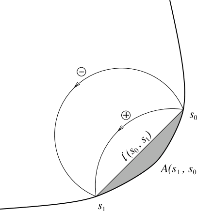
Figure 13: Geometry of the trajectories for a convex billiard in strong magnetic field.

We now proceed to the proof of the proposition.

Choose two points $P$ and $P^{\prime}$ on $\partial Q$. They can be connected by two, one or no arc of trajectory, depending on whether their distance is smaller than, equal to, or larger than $2\mu$. In each of the first two cases, we call $s_{0}$ and $s_{1}$ their abscissas, as in figure 13. We define

$$\sigma=\frac{(s_{0}-s_{1})\pmod{\left|\partial Q\right|}}{\mu}.$$ (96)

The corollary and our sign conventions imply that $0<\sigma<\pi$. Moreover, the arcs cannot intersect $\partial Q$ at a point different from $P$ or $P^{\prime}$.

Following the proof of proposition 2, it is easy to show that the two trajectories can be described by the generating functions

$$G^{\pm}(s_{0},s_{1})=-\frac{1}{\mu}A(s_{1},s_{0})\pm\mu b\left(\frac{\ell(s_{0},s_{1})}{2\mu}\right),$$ (97)

in the sense that $dG^{\pm}=u_{0}^{\pm}ds_{0}-u_{1}^{\pm}ds_{1}$. Here, $\ell\in(0,2\mu]$ and $A$ are defined in fig.13, and

$$b(x) = {\mbox{$\rm Arcsin$}}x+x\sqrt{1-x^{2}}$$

$$b^{\prime}(x) = 2\sqrt{1-x^{2}}.$$ (98)

The functions $A$ and $\ell$ are directly related to the shape of $\partial Q$, that we describe using the function $\tau(s)$, which has the properties

1. $\tau(s+\left|\partial Q\right|)=\tau(s)+2\pi$,

2. $\tau^{\prime}(s)=\kappa(s)\in[\frac{1}{\rho_{\mathchoice{\mbox{$\displaystyle\rm max$}}{\mbox{$\textstyle\rm max$}}{\mbox{$\scriptstyle\rm max$}}{\mbox{$\scriptscriptstyle\rm max$}}}},\frac{1}{\rho_{\mathchoice{\mbox{$\displaystyle\rm min$}}{\mbox{$\textstyle\rm min$}}{\mbox{$\scriptstyle\rm min$}}{\mbox{$\scriptscriptstyle\rm min$}}}}]$,

3. $\displaystyle\int_{0}^{\left|\partial Q\right|}\mathchoice{\mbox{$\displaystyle\rm e$}}{\mbox{$\textstyle\rm e$}}{\mbox{$\scriptstyle\rm e$}}{\mbox{$\scriptscriptstyle\rm e$}}^{\mathchoice{\mbox{$\displaystyle\rm i$}}{\mbox{$\textstyle\rm i$}}{\mbox{$\scriptstyle\rm i$}}{\mbox{$\scriptscriptstyle\rm i$}}\tau(s)}ds=0$.

If $\mathchoice{\mbox{\boldmath$\displaystyle\bf\ell$}}{\mbox{\boldmath$\textstyle\bf\ell$}}{\mbox{\boldmath$\scriptstyle\bf\ell$}}{\mbox{\boldmath$\scriptscriptstyle\bf\ell$}}(s_{0},s_{1})$ is the vector connecting the points of abscissas $s_{0}$ and $s_{1}$, we have

$${\mbox{\boldmath$\bf\ell$}}(s_{0},s_{1}) = \int_{s_{0}}^{s_{1}}\mathchoice{\mbox{\boldmath$\displaystyle\bf t$}}{\mbox{\boldmath$\textstyle\bf t$}}{\mbox{\boldmath$\scriptstyle\bf t$}}{\mbox{\boldmath$\scriptscriptstyle\bf t$}}(s)ds$$

$$\ell(s_{0},s_{1})^{2} = \int_{s_{0}}^{s_{1}}ds\int_{s_{0}}^{s_{1}}ds^{\prime}\left(\mathchoice{\mbox{\boldmath$\displaystyle\bf t$}}{\mbox{\boldmath$\textstyle\bf t$}}{\mbox{\boldmath$\scriptstyle\bf t$}}{\mbox{\boldmath$\scriptscriptstyle\bf t$}}(s)|\mathchoice{\mbox{\boldmath$\displaystyle\bf t$}}{\mbox{\boldmath$\textstyle\bf t$}}{\mbox{\boldmath$\scriptstyle\bf t$}}{\mbox{\boldmath$\scriptscriptstyle\bf t$}}(s^{\prime})\right)=\int_{s_{0}}^{s_{1}}ds\int_{s_{0}}^{s_{1}}ds^{\prime}\cos\left[\tau(s)-\tau(s^{\prime})\right]$$

$$A(s_{0},s_{1}) = \int_{s_{0}}^{s_{1}}ds\frac{1}{2}\left|\mathchoice{\mbox{\boldmath$\displaystyle\bf\ell$}}{\mbox{\boldmath$\textstyle\bf\ell$}}{\mbox{\boldmath$\scriptstyle\bf\ell$}}{\mbox{\boldmath$\scriptscriptstyle\bf\ell$}}(s_{0},s)\wedge\mathchoice{\mbox{\boldmath$\displaystyle\bf t$}}{\mbox{\boldmath$\textstyle\bf t$}}{\mbox{\boldmath$\scriptstyle\bf t$}}{\mbox{\boldmath$\scriptscriptstyle\bf t$}}(s)\right|=\frac{1}{2}\int_{s_{0}}^{s_{1}}ds\int_{s_{0}}^{s}ds^{\prime}\sin\left[\tau(s)-\tau(s^{\prime})\right].$$ (99)

Carrying out the change of variables $s=s_{0}+\mu\sigma t$, we obtain $\ell(s_{0},s_{1})^{2}=\mu^{2}\sigma^{2}I(s_{0},\mu\sigma)$, $A(s_{1},s_{0})=\frac{1}{2}\mu^{2}\sigma^{2}I^{\prime}(s_{0},\mu\sigma)$, where

$$I(s_{0},\mu\sigma) = \int_{-1}^{0}dt\int_{-1}^{0}dt^{\prime}\cos T(s_{0},\mu\sigma t,\mu\sigma t^{\prime})$$

$$I^{\prime}(s_{0},\mu\sigma) = \int_{-1}^{0}dt\int_{-1}^{t}dt^{\prime}\sin T(s_{0},\mu\sigma t,\mu\sigma t^{\prime})$$

$$T(s_{0},\mu\sigma t,\mu\sigma t^{\prime}) = \tau(s_{0}+\mu\sigma t)-\tau(s_{0}+\mu\sigma t^{\prime}).$$ (100)

If the boundary is $C^{2}$, one gets $T=O(\mu\sigma)$, $I=1+O(\mu\sigma)$, $I^{\prime}=O(\mu\sigma)$, and thus $G^{\pm}(s_{0},s_{1},\mu)=\mu g^{\pm}(\sigma,s_{0},\mu)$, where $g^{\pm}(\sigma,s_{0},0)=\pm b\left(\frac{\sigma}{2}\right)$ does not depend on $s_{0}$. From this fact, we can already guess the structure of the map. Indeed, $u_{0}^{\pm}=\partial_{\sigma}g^{\pm}+\mu\partial_{s_{0}}g^{\pm},u_{1}^{\pm}=\partial_{\sigma}g^{\pm}$, and thus $u_{1}^{\pm}=u_{0}^{\pm}+\mu\partial_{s_{0}}g^{\pm}=u_{0}^{\pm}+O(\mu^{2})$.

However, $G$ is not sufficiently smooth around $\ell=2\mu$ to be expanded. We proceed in a slightly different way: taking derivatives of (99), we obtain

$$\frac{\partial\ell}{\partial s_{0}}=\frac{\mu}{\ell}\sigma J,\;\;\;\frac{\partial A}{\partial s_{0}}=\frac{\mu}{2}\sigma K,\;\;\;\frac{\partial A}{\partial s_{1}}=-\frac{\mu}{2}\sigma K^{\prime},$$ (101)

where

$$J(s_{0},\mu\sigma) = \int_{-1}^{0}dt\cos T(s_{0},0,\mu\sigma t)$$

$$K(s_{0},\mu\sigma) = \int_{-1}^{0}dt\sin T(s_{0},0,\mu\sigma t)$$

$$K^{\prime}(s_{0},\mu\sigma) = \int_{-1}^{0}dt\cos T(s_{0},\mu\sigma t,-\mu\sigma).$$ (102)

Note that if the boundary is $C^{k}$, the above integrals are all $C^{k-1}$. Differentiating (97), we get

$$u_{0}^{\pm}=\frac{\partial G^{\pm}}{\partial s_{0}}=\pm\sqrt{1-\frac{\ell^{2}}{4\mu^{2}}}\;\frac{\partial\ell}{\partial s_{0}}-\frac{1}{\mu}\frac{\partial A}{\partial s_{0}}=\pm\sqrt{1-\frac{1}{4}\sigma^{2}I}\;\frac{\mu}{\ell}\sigma J-\frac{1}{2}\sigma K$$

$$\left(u_{0}+\frac{1}{2}\sigma K\right)^{2} = \left(1-\frac{1}{4}\sigma^{2}I\right)\frac{J^{2}}{I}$$

$$4I(1-u_{0}^{2})=4I\sin^{2}\theta_{0} = \sigma^{2}(K^{2}+J^{2})I-4\sigma\cos\theta_{0}KI+4(I-J^{2})$$ (103)

$$= \Phi_{0}(\sigma,\mu,s_{0},\theta_{0}).$$

When the boundary is $C^{3}$, we have $I=1+O(\mu^{2}\sigma^{2})$, $J=1+O(\mu^{2}\sigma^{2})$ and $K=\frac{1}{2}\kappa(s_{0})\mu\sigma+O(\mu^{2}\sigma^{2})$, so that $\Phi_{0}=\sigma^{2}\left[1-2\cos\theta_{0}\kappa(s_{0})\mu+O(\mu^{2})\right]$.

If we write $\sigma=2\sin\theta_{0}\eta$, then

$$0=\Phi(\eta,\mu,s_{o},\theta_{0})=\left.\left[\sqrt{I}-\eta\sqrt{\frac{\Phi_{0}}{\sigma^{2}}}\,\right]\right|_{\sigma=2\sin\theta_{0}\eta}=1-\eta\left[1-\cos\theta_{0}\kappa(s_{0})\mu+O(\mu^{2})\right].$$ (104)

The function $\Phi$ has the properties $\Phi(\eta_{0},0,s_{0},\theta_{0})=0$, where $\eta_{0}=1$, and $\partial_{\eta}\Phi(\eta_{0},0,s_{0},\theta_{0})=-1$. Thus, the implicit function theorem implies that in a neighborhood of $\mu=0$, $\eta$ can be expressed as a $C^{k-1}$ function of $\mu,s_{0}$ and $\theta_{0}$. This function can be constructed using Newton’s method: if $\eta_{0}\equiv 1$ and $\eta_{n+1}(s_{0},\theta_{0},\mu)=\eta_{n}(s_{0},\theta_{0},\mu)+\Phi(\eta_{n}(s_{0},\theta_{0},\mu),\mu,s_{0},\theta_{0})$, then $\Phi(\eta_{n},\mu,s_{0},\theta_{0})=O(\mu^{n+1})$. For $k=3$, we get

$$\eta(s_{0},\theta_{0},\mu)=1+\cos\theta_{0}\kappa(s_{0})\mu+O(\mu^{2}).$$ (105)

The first equation of (41) is obtained by using $s_{1}=s_{0}-\mu\sigma=s_{0}-2\mu\sin\theta_{0}\eta$, i.e.

$$a(s_{0},\theta_{0},\mu)=\frac{2}{\mu}(1-\eta(s_{0},\theta_{0},\mu))\in C^{k-2}.$$ (106)

Note that if we had used the variable $u$ instead of $\theta$, we would not have been able to apply the implicit function theorem when $u\rightarrow\pm 1$. Indeed, the map expressed in the variables $(u,s)$ contains the factor $\sqrt{1-u_{0}^{2}}$.

To obtain the second equation of (41), we observe that (see (86)):

$$\theta_{1}-\theta_{0} = (\theta_{1}+\chi)-(\theta_{0}+\chi)$$ (107)

$$= \left[\pi-\mathchoice{\mbox{$\displaystyle\rm Arcsin$}}{\mbox{$\textstyle\rm Arcsin$}}{\mbox{$\scriptstyle\rm Arcsin$}}{\mbox{$\scriptscriptstyle\rm Arcsin$}}\left(\frac{2}{\ell}\frac{\partial A}{\partial s_{1}}\right)\right]-\left[\pi-\mathchoice{\mbox{$\displaystyle\rm Arcsin$}}{\mbox{$\textstyle\rm Arcsin$}}{\mbox{$\scriptstyle\rm Arcsin$}}{\mbox{$\scriptscriptstyle\rm Arcsin$}}\left(-\frac{2}{\ell}\frac{\partial A}{\partial s_{0}}\right)\right]$$

$$= {\mbox{$\rm Arcsin$}}\left(\frac{K}{\sqrt{I}}\right)-\mathchoice{\mbox{$\displaystyle\rm Arcsin$}}{\mbox{$\textstyle\rm Arcsin$}}{\mbox{$\scriptstyle\rm Arcsin$}}{\mbox{$\scriptscriptstyle\rm Arcsin$}}\left(\frac{K^{\prime}}{\sqrt{I}}\right)=O(\mu^{2}\sigma^{2}),$$

where we have used point 4 of the corollary to choose the determination of $\textstyle\rm Arcsin$. By consequence,

$$b(s_{0},\theta_{0},\mu)=\left.\frac{4\eta^{2}}{\mu^{2}\sigma^{2}}\left[\mathchoice{\mbox{$\displaystyle\rm Arcsin$}}{\mbox{$\textstyle\rm Arcsin$}}{\mbox{$\scriptstyle\rm Arcsin$}}{\mbox{$\scriptscriptstyle\rm Arcsin$}}\left(\frac{K}{\sqrt{I}}\right)-\mathchoice{\mbox{$\displaystyle\rm Arcsin$}}{\mbox{$\textstyle\rm Arcsin$}}{\mbox{$\scriptstyle\rm Arcsin$}}{\mbox{$\scriptscriptstyle\rm Arcsin$}}\left(\frac{K^{\prime}}{\sqrt{I}}\right)\right]\right|_{\sigma=2\sin\theta_{0}\eta}\in C^{k-3}.$$ (108)

Higher orders of the expansions of $a$ and $b$ can be obtained by computing expansions of $I,J,K,K^{\prime}$ and $\eta$ up to the desired order, and replacing them in (106) and (108).     $\sqcap$$\sqcup$

Appendix E Symmetric orbits of period $4k$ in the square

We want to study existence and stability of $4k$-periodic trajectories, similar to the one shown in figure 7f, where $k=2$. As shown in figure 14, such trajectories can be characterized by numbers $x$, $y$ or $x^{\prime}$, $y^{\prime}$, satisfying

$$\begin{array}[]{ll}\left\{\begin{array}[]{l}2kx+2(k+1)y=1\\ 2y^{2}+2xy+x^{2}=\mu^{2},\end{array}\right.\phantom{MM}&\left\{\begin{array}[]{l}0\leq y<\frac{1}{2}\\ 0\leq 2y+x\leq\frac{1}{2},\end{array}\right.\\ \\ \left\{\begin{array}[]{l}2kx^{\prime}+2(k-1)y^{\prime}=1\\ 2y^{\prime 2}+2x^{\prime}y^{\prime}+x^{\prime 2}=\mu^{2},\end{array}\right.&\left\{\begin{array}[]{l}0\leq y^{\prime}\\ 0<x^{\prime}\leq\frac{1}{2}.\end{array}\right.\end{array}$$ (109)

Figure 14: Geometry of symmetric $4k$-periodic trajectories in the square.

These equations have 3 different kinds of solutions:

$$\begin{array}[]{lcll}y_{+}&=&\displaystyle\frac{1+R}{2(k^{2}+1)},\phantom{MMM}&\mu_{k}^{-}\leq\mu<\displaystyle\frac{1}{2},\\ &&&\\ y_{-}&=&\displaystyle\frac{1-R}{2(k^{2}+1)},&\mu_{k}^{-}\leq\mu\leq\displaystyle\frac{1}{2k},\\ &&&\\ y^{\prime}&=&\displaystyle\frac{-1+R}{2(k^{2}+1)},&\displaystyle\frac{1}{2k}\leq\mu<\displaystyle\frac{1}{\sqrt{2}(k-1)},\\ \end{array}$$ (110)

where

$$R=\displaystyle\sqrt{1-(k^{2}+1)(1-4k^{2}\mu^{2})},\;\;\;\mu_{k}^{-}=\displaystyle\frac{1}{2\sqrt{k^{2}+1}}.$$ (111)

Using (3), we find that the stability matrix for $k$ bounces is

$$S_{k} = \left(\begin{array}[]{cc}C&\mu(1-C^{2})\\ -\frac{1}{\mu}&C\end{array}\right)\left(\begin{array}[]{cc}1&-2\mu C\\ 0&1\end{array}\right)^{k-1}=\left(\begin{array}[]{cc}C&\mu(1-(2k-1)C^{2})\\ -\frac{1}{\mu}&(2k-1)C\end{array}\right),$$ (118)

$$t = \frac{1}{2}\mathchoice{\mbox{$\displaystyle\rm Tr$}}{\mbox{$\textstyle\rm Tr$}}{\mbox{$\scriptstyle\rm Tr$}}{\mbox{$\scriptscriptstyle\rm Tr$}}S_{k}=Ck,$$ (119)

where

$$C=\mathchoice{\mbox{$\displaystyle\rm cotg$}}{\mbox{$\textstyle\rm cotg$}}{\mbox{$\scriptstyle\rm cotg$}}{\mbox{$\scriptscriptstyle\rm cotg$}}\theta=\frac{y}{y+x}=-\frac{y^{\prime}}{y^{\prime}+x^{\prime}}.$$ (120)

Now, since

$$S_{4k}=S_{k}^{4},\;\;\;\frac{1}{2}\mathchoice{\mbox{$\displaystyle\rm Tr$}}{\mbox{$\textstyle\rm Tr$}}{\mbox{$\scriptstyle\rm Tr$}}{\mbox{$\scriptscriptstyle\rm Tr$}}S_{4k}=8t^{4}-8t^{2}+1,$$ (121)

the total orbit is hyperbolic if $\left|t\right|>1$, parabolic if $\left|t\right|=0,\frac{1}{\sqrt{2}},1$, and elliptic otherwise. Applying this to (119), we find that $y_{+}$-orbits are hyperbolic as soon as $\mu>\mu_{k}^{-}$, $y_{-}$-orbits are never hyperbolic, and $y^{\prime}$-orbits are hyperbolic if $\mu>\mu_{k}^{+}$, where

$$\mu_{k}^{+}=\frac{\sqrt{k^{2}+1}}{2(k^{2}-1)}.$$ (122)

We have thus obtained that symmetric $4k$-periodic orbits may be stable only if $\mu_{k}^{-}<\mu<\mu_{k}^{+}$. These bounds have the properties

$$\begin{array}[]{rcccl}\mu_{k}^{-}&<&\displaystyle\frac{1}{2k}&<&\mu_{k}^{+},\\ &&&&\\ \mu_{k-1}^{-}&>&\mu_{k}^{+}&&\mbox{if }\;k>2.\end{array}$$

We see that when $\mu<\mu_{k}^{-}$, no $4k$-periodic orbit exists. At $\mu=\mu_{k}^{-}$, a pair of such orbits with opposite stability appears in a saddle-node bifurcation. The stable one loses stability at $\mu=\mu_{k}^{+}$. Numerical simulations show that new stable orbits are created, but they quickly loose stability for some $\mu=\mu_{k}^{*}$. For $k>2$, this happens long before a $4(k-1)$-periodic orbit appears at $\mu=\mu_{k-1}^{-}$, and since no other stable orbits can be found in the interval, we are lead to the conjecture that the billiard in a square is ergodic when $\mu_{k}^{*}\leq\mu\leq\mu_{k-1}^{-}$.

Appendix F Elliptic orbits of period 6 outside 2 circles

We want to show that the billiard outside 2 circles described in section 6.2 possesses elliptic orbits for some values of the parameters.

The trajectory depicted in figure 10b for $\mu=\lambda=1$ turns out to be linearly marginally stable for these values of the parameters if we apply (3). Thus we have to analyse its stability for nearby value of $\mu$ and $\lambda$.

Figure 15: Geometry of period 6 trajectories outside 2 circles. We show a quarter of the trajectory, which is symmetric with respect to the coordinate axes.

The trajectory can be characterized by two angles $\theta^{\prime}$ and $\varphi$, as in figure 15. The other angles are then given by $\chi_{1}=\frac{\pi}{2}+\theta^{\prime}-\frac{\varphi}{2}$, $\chi_{2}=\theta^{\prime}+\varphi-\frac{\pi}{2}$. Using the relations $\mu\sin\chi_{1}=\sin\left(\frac{\pi-\varphi}{2}\right)$ and $\cos\varphi+\mu\sin\chi_{2}=\lambda$, we obtain the system

$$\left\{\begin{array}[]{l}1+\cos\varphi=\mu^{2}(1+\cos(\varphi-2\theta^{\prime}))\\ \cos\varphi-\mu\cos(\varphi+\theta^{\prime})=\lambda.\end{array}\right.$$ (123)

For small values of $\varepsilon=\mu-1$ and $\delta=\lambda-1$, it has the solution

$$\left\{\begin{array}[]{rcl}\theta^{\prime}&=&\displaystyle\frac{\pi}{3}-\displaystyle\frac{1}{\sqrt{3}}\varepsilon+\displaystyle\frac{1}{\sqrt{3}}\delta+O(2)\phantom{\displaystyle\frac{1}{\displaystyle\frac{1}{2}}}\\ \varphi&=&\displaystyle\frac{\pi}{3}-\frac{4}{\sqrt{3}}\varepsilon+\frac{1}{\sqrt{3}}\delta+O(2),\end{array}\right.$$ (124)

where $O(2)$ stands for terms of order $\varepsilon^{2}$, $\delta^{2}$, $\varepsilon\delta$. The Jacobian matrices $M_{1}$ and $M_{2}$ for the two types of bounces can now be computed using (3), with $\theta_{i}=\pi-\theta^{\prime}$ and $\ell_{i}\cos\chi_{i}=\mu\sin(2\chi_{i})$. The stability matrix of the orbit is given by $S_{6}=(S_{3})^{2}$, $S_{3}=M_{1}^{2}M_{2}$. We obtain

$$t = \frac{1}{2}\mathchoice{\mbox{$\displaystyle\rm Tr$}}{\mbox{$\textstyle\rm Tr$}}{\mbox{$\scriptstyle\rm Tr$}}{\mbox{$\scriptscriptstyle\rm Tr$}}S_{3}=-1-12\varepsilon+6\delta+O(2),$$

$$\Rightarrow\frac{1}{2}\mathchoice{\mbox{$\displaystyle\rm Tr$}}{\mbox{$\textstyle\rm Tr$}}{\mbox{$\scriptstyle\rm Tr$}}{\mbox{$\scriptscriptstyle\rm Tr$}}S_{6} = 2t^{2}-1=1+48\varepsilon-24\delta+O(2).$$ (125)

Hence, for small $\delta$ and $\varepsilon$, the orbit is elliptic for $\delta>2\varepsilon+O(\varepsilon^{2})$, i.e. for $\lambda>2\mu-1+O((\mu-1)^{2})$, in a neighbourhood of $\lambda=\mu=1$.

References

- [A1] V.I. Arnold, Mathematical Methods of Classical Mechanics, (Springer, 1978, 1989).
- [A2] V.I. Arnold, Geometrical Methods in the Theory of Ordinary Differential Equations, (Springer, 1983).
- [B] G.D. Birkhoff, Dynamical Systems, (Amer. Math. Soc., 1927, 1966).
- [Do] R. Douady, Applications du théorème des tores invariants, Thèse cycle, Univ. Paris VII (1982).
- [DR] T. Dagaeff, C. Rouvinez, On the discontinuities of the boundary in billiards, Physica D 67, 166-187 (1993).
- [H] A. Hubacher, Instability of the Boundary in the Billiard Ball Problem, Commun. Math. Phys. 108, 483-488 (1987).
- [KT] V.V. Kozlov, D.V. Treshchev, Billiards: a genetic introduction to the dynamics of systems with impacts, (Amer. Math. Soc., 1991).
- [L] V.F. Lazutkin, The existence of caustics for a billiard ball problem in a convex domain, Math. USSR Izvestija 7, 185-214 (1973), translation of Izv. Akad. Nauk SSSR 37, 1973.
- [LRPW] L.P. Lévy, D.H. Reich, L. Pfeiffer, K. West, Aharonov-Bohm ballistic billiards, Physica B 189, 204 (1993).
- [Ma] J.N. Mather, Glancing billiards, Ergod. Th. & Dynam. Sys. 2, 397-403 (1982).
- [Me] J.D. Meiss, Symplectic maps, variational principles, and transport, Rev. Mod. Phys. 64, 795-848 (1992).
- [Mo] J. Moser, Stable and Random Motions in Dynamical Systems, (Princeton Univ. Press, 1973).
- [MBG] O. Meplan, F. Brut, C. Gignoux, Tangent map for classical billiards in magnetic fields, J. Phys. A 26, 237-246 (1993).
- [Ro] M. Robnik, Regular and Chaotic Billiard Dynamics in Magnetic Fields, in Nonlinear Phenomena and Chaos, ed. S. Sakar, (Adam Hilger, 1986), pp 303-330.
- [RB] M. Robnik, M.V. Berry, Classical billiards in magnetic fields, J. Phys. A 18, 1361-1378 (1985).
- [RKC] K. Rezakhanlou, H. Kunz, A. Crisanti, Stochastic Behaviour of the Magnetisation in a Classically Integrable Quantum System, Europhys. Lett. 16, 629-634 (1991).